Lifted Explanations
∗
Arun Nampally
1and C. R. Ramakrishnan
21 Computer Science Dept., Stony Brook University, Stony Brook, NY, USA
2 Computer Science Dept., Stony Brook University, Stony Brook, NY, USA
Abstract
In this paper, we consider the problem of lifted inference in the context of Prism-like probabilistic logic programming languages. Traditional inference in such languages involves the construction of an explanation graph for the query that treats each instance of a random variable separately. For many programs and queries, we observe that explanations can be summarized into substantially more compact structures introduced in this paper, called “lifted explanation graphs”. In contrast to existing lifted inference techniques, our method for constructing lifted explanations naturally generalizes existing methods for constructing explanation graphs. To compute probability of query answers, we solve recurrences generated from the lifted graphs. We show examples where the use of our technique reduces the asymptotic complexity of inference.
1998 ACM Subject Classification D.1.6 Logic Programming, D.3.3 Language Constructs and Features – Constraints,F.3.2 Semantics of Programming Languages – Operational semantics, I.2.3 Deduction and Theorem Proving – Logic programming, Resolution, Uncertain, “fuzzy”, and probabilistic reasoning
Keywords and phrases Probabilistic logic programs, Probabilistic inference, Lifted inference, Symbolic evaluation, Constraints
Digital Object Identifier 10.4230/OASIcs.ICLP.2016.15
1
Introduction
Probabilistic Logic Programming (PLP) provides a declarative programming framework to specify and use combinations of logical and statistical models. A number of programming languages and systems have been proposed and studied under the framework of PLP, e.g. PRISM [12], Problog [4], PITA [11] and Problog2 [5] etc. These languages have similar declarative semantics based on thedistribution semantics[13]. The inference algorithms used in many of these systems to evaluate the probability of query answers, e.g. PRISM, Problog and PITA, are based on a common notion ofexplanation graphs. These graphs represent explanations, which are sets ofprobabilistic choicesthat are abduced during query evaluation. Explanation graphs are implemented differently by different systems; e.g. PRISM uses tables to represent them undermutual exclusion andindependenceassumptions on explanations; ProbLog and PITA represents them using Binary Decision Diagrams (BDDs).
Inference based on explanation graphs does not scale well to logical/statistical models with large numbers of random processes and variables. In particular, in models containingfamilies
∗ This work was supported in part by NSF grants IIS 1447549 and CNS 1405641.
© Arun Nampally and C. R. Ramakrishnan; licensed under Creative Commons License CC-BY
1% Two distinct tosses show "h" 2twoheads :-3 X in coins, 4 msw(toss, X, h), 5 Y in coins, 6 {X < Y}, 7 msw(toss, Y, h). 8 9% Cardinality of coins: 10:- population(coins, 100). 11 12% Distribution parameters: 13:- set_sw(toss, 14categorical([h:0.5, t:0.5])). (toss,1) (toss,2) (toss,2) (toss, n−1) (toss,3) 1 0 (toss, n) 1 0 1 t h t h t h t h t h t h ∃X.∃Y.X<Y (toss,X) (toss,Y) 0 1 0 h t h t
(a) Simple Px program (b) Ground expl. Graph (c) Lifted expl. Graph
Figure 1Example program and ground explanation graph.
of independent, identically distributed (i.i.d) random variables, outcomes of individual random variables are abduced. However, as developments in the area oflifted inference [10, 2, 7] have shown, vast savings in computational effort can be made by exploiting the symmetry in models with populations of i.i.d random variables. The lifted inference algorithms seek to treat a set of i.i.d random variables as single unit and aggregate their behavior to achieve computational speedup. This paper presents a structure for representing explanation graphs compactly by exploiting the symmetry with respect to i.i.d random variables, and a procedure to build this structure without enumerating each instance of a random process.
Illustration. The simple example in Fig. 1 shows a program describing a process of tossing a number of i.i.d. coins, and evaluating if at least two of them came up “heads”. The example is specified in an extension of the PRISM language, called Px. Explicit random processes of PRISM enables a clearer exposition of our approach. In PRISM and Px, a special predicate of the formmsw(p, i, v)describes, given a random processpthat defines a family of i.i.d. random variables, thatv is the value of the i-th random variable in the family. The argumentiofmswis called the ithinstanceargument. In this paper, we consider Param-Px, a further extension of Px to define parameterized programs. In Param-Px, a built-in predicate,inis used to specify membership; e.g. x in smeansxis member of an enumerable sets. The size ofsis specified by a separatepopulationdirective. The program in Fig. 1 defines a family of random variables generated bytoss. The instances that index these random variables are drawn from the setcoins. Finally, predicatetwoheadsis defined to hold if tosses of at least two distinct coins come up “h”.
State of the Art, and Our Solution. Inference in PRISM, Problog and PITA follows the structure of the derivations for a query. Consider the program in Fig. 1(a) and let the cardinality of the set of coins ben. The query twoheadswill take Θ(n2) time, since it will
construct bindings to bothXandYin the clause definingtwoheads. However, the size of an explanation graph is Θ(n), as shown in Fig. 1(b). Computing the probability of the query over this graph will also take Θ(n) time.
In this paper, we present a technique to construct a symbolic version of an explanation graph, called alifted explanation graphthat represents instances symbolically and avoids enumerating the instances of random processes such astoss. The lifted explanation graph for querytwoheadsis shown in Fig. 1(c). Unlike traditional explanation graphs where nodes are specific instances of random variables, nodes in the lifted explanation graph may be parameterized by their instance (e.g (toss, X) instead of (toss,1)). A set of constraints on
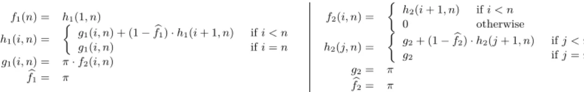
f1(n) = h1(1, n) h1(i, n) = g1(i, n) + (1−fb1)·h1(i+ 1, n) ifi < n g1(i, n) ifi=n g1(i, n) = π·f2(i, n) b f1= π f2(i, n) = h2(i+ 1, n) ifi < n 0 otherwise h2(j, n) = g2+ (1−fb2)·h2(j+ 1, n) ifj < n g2 ifj=n g2= π b f2= π
Figure 2Recurrences for computing probabilities for Example in Fig. 1.
those variables, specify the allowed groundings.
Note that the graph size is independent of the size of the population. Moreover, the graph can be constructed in time independent of the population size as well. Probability computation is performed by first deriving recurrences based on the graph’s structure and then solving the recurrences. The recurrences for probability computation derived from the graph in Fig. 1(c) are shown in Fig. 2. In the figure, the equations with subscript 1 are derived from the root of the graph; those with subscript 2 from the left child of the root; and whereπis the probability thattossis “h”. Note that the probability of the query,f1(n),
can be computed in Θ(n) time from the recurrences.
Contributions. The technical contribution of this paper is two fold.
1. We define a lifted explanation structure, and operations over these structures (see Section 3). We also give method to construct such structures during query evaluation, closely following the techniques used to construct explanation graphs.
2. We define a technique to compute probabilities over such structures by deriving and solving recurrences (see Section 4). We provide examples to illustrate the complexity gains due to our technique over traditional inference.
The rest of the paper begins by defining parameterized Px programs and their semantics (Section 2). After presenting the main technical work, the paper concludes with a discussion
of related work. (Section 5).
2
Parameterized Px Programs
The PRISM language follows Prolog’s syntax. It adds a binary predicatemswto introduce random variables into an otherwise familiar Prolog program. Specifically, in msw(s, v),sis a “switch” that represents a random process which generates a family of random variables, andv is bound to the value of a variable in that family. The domain and distribution of the switches are specified byset_swdirectives. Given a switchs, we use Ds to denote the domain ofs, andπs:Ds→[0,1] to denote its probability distribution.
2.1
Px and Inference
The Px language extends the PRISM language in three ways. Firstly, themswswitches in Px are ternary, with the addition of an explicit instanceparameter. This brings the language closer to the formalism presented when describing PRISM’s semantics [13]. Secondly, Px aims to compute the distribution semantics without themutual exclusion andindependence assumptions on explanations imposed by PRISM system. Thirdly, in contrast to PRISM, the switches in Px can be defined with a wide variety of univariate distributions, including continuous distributions (such as Gaussian) and infinite discrete distributions (such as Poisson). However, in this paper, we consider only programs with finite discrete distributions.
Exact inference of Px programs with finite discrete distributions uses explanation graphs with the following structure.
IDefinition 1 (Ground Explanation Graph). Let S be the set of ground switches in a Px programP, and Ds be the domain of switch s∈S. LetT be the set of all ground terms over symbols inP. Let “≺” be a total order overS× T such that (s1, t1)≺(s2, t2) if either t1< t2ort1=t2 ands1< s2. Aground explanation treeoverP is a rooted treeγsuch that:
Leaves inγ are labeled 0 or 1.
Internal nodes inγare labeled (s, z) wheres∈S is a switch, andzis a ground term over symbols inP.
For node labeled (s, z), there arek outgoing edges to subtrees, where k=|Ds|. Each edge is labeled with a uniquev∈Ds.
Let (s1, z1),(s2, z2), . . . ,(sk, zk), cbe the sequence of node labels in a root-to-leaf path in the tree, wherec∈ {0,1}. Then (si, zi)≺(sj, zj) ifi < j for alli, j≤k. As a corollary, node labels along any root to leaf path in the tree are unique.
Anexplanation graph is a DAG representation of a ground explanation tree.
Consider a sequence of alternating node and edge labels in a root-to-leaf path: (s1, z1), v1,(s2, z2), v2, . . . ,(sk, zk), vk, c. Each such path enumerates a set of random variable valuations{s1[z1] =v1, s2[z2] =v2, . . . , sk[zk] =vk}. Whenc= 1, the set of valuations forms an explanation. An explanation graph thus represents a set of explanations.
Note that explanation trees and graphs resemble decision diagrams. Indeed, explanation graphs are implemented using Binary Decision Diagrams [3] in PITA and Problog; and Multi-Valued Decision Diagrams [15] in Px. Theunion of two sets of explanations can be seen as an “or” operation over corresponding explanation graphs. Pair-wise union of explanations in two sets is an “and” operation over corresponding explanation graphs.
2.1.1
Inference via Program Transformation
Inference in Px is performed analogous to that in PITA [11]. Concretely, inference is done by translating a Px program to one that explicitly constructs explanation graphs, performing tabled evaluation of the derived program, and computing probability of answers from the explanation graphs. We describe the translation for definite pure programs; programs with built-ins and other constructs can be translated in a similar manner.
For every user-defined atomAof the formp(t1, t2, . . . , tn), we defineexp(A, E) as atom
p(t1, t2, . . . , tn, E) with a new predicate p/(n+ 1), with E as an added “explanation” ar-gument. For such atoms A, we also define head(A, E) as atom p0(t1, t2, . . . , tn, E) with a new predicate p0/(n+ 1). A goal G is a conjunction of atoms, where G = (G
1, G2)
for goals G1 and G2, or G is an atom A. Function exp is extended to goals such that
exp((G1, G2)) = ((exp(G1, E1),exp(G2, E2)),and(E1, E2, E)), whereandis a predicate in the
translated program that combines two explanations using conjunction, andE1 andE2 are
fresh variables. Functionexp is also extended tomswatoms such thatexp(msw(p, i, v), E) is
rv(p, i, v, E), wherervis a predicate that bindsEto an explanation graph with root labeled
(p, i) with an edge labeledvleading to a 1 child, and all other edges leading to 0.
Each clause of the form A :−G in a Px program is translated to a new clause head(A, E) :−exp(G, E). For each predicate p/n, we define p(X1, X2, . . . Xn, E) to be such thatE is the disjunction of allE0 forp0(X1, X2, . . . Xn, E0). As in PITA, this is done using answer subsumption.
Probability of an answer is determined by first materializing the explanation graph, and then computing the probability over the graph. The probability associated with a node in
the graph is computed as the sum of the products of probabilities associated with its children and the corresponding edge probabilities. The probability associated with an explanation graphϕ, denotedprob(ϕ) is the probability associated with the root. This can be computed in time linear in the size of the graph by using dynamic programming or tabling.
2.2
Syntax and Semantics of Parameterized Px Programs
Parameterized Px, called Param-Px for short, is a further extension of the Px language. The first feature of this extension is the specification ofpopulations andinstances to specify ranges of instance parameters of msws.
IDefinition 2(Population). Apopulation is a named finite set, with a specified cardinality. A population has the following properties:
1. Elements of a population may be atomic, or depth-bounded ground terms.
2. Elements of a population are totally ordered using the default term order.
3. Distinct populations are disjoint.
Populations and their cardinalities are specified in a Param-Px program by population
facts. For example, the program in Figure 1(a) defines a population namedcoinsof size 100. The individual elements of this set are left unspecified. When necessary,element/2facts may be used to define distinguished elements of a population. For example,element(fred, persons) defines a distinguished element “fred” in population persons. In presence of
elementfacts, elements of a population are ordered as follows. The order of elementfacts specifies the order among the distinguished elements, and all distinguished elements occur before other unspecified elements in the order.
IDefinition 3(Instance). Aninstanceis an element of a population. In a Param-Px program, a built-in predicatein/2 can be used to draw an instance from a population. All instances of a population can be drawn by backtracking over in.
An instance variable is one that occurs as the instance argument in a mswpredicate in a clause of a Param-Px program. In Fig. 1(a),X in coinsbindsXto an instance of population
coinsandX,Yare instance variables.
Constraints. The second extension in Param-Px are atomic constraints, of the form{t1= t2},{t16=t2}and{t1< t2}, wheret1andt2are variables or constants, to compare instances
of a population. We use braces “{·}” to distinguish the constraints from Prolog built-in comparison operators. In Figure 1(a),{X \= Y}is an atomic constraint.
Types. We use populations in a Param-Px program to confer types to program variables. Each variable that occurs in an “in” predicate is assigned a unique type. More specifically,
X has typepif X in poccurs in a program, wherepis a population; and X is untyped otherwise. We extend this notion of types to constants and switches as well. A constantc
has typepif there is a factelement(c, p); andcis untyped otherwise. A switchshas type
pif there is anmsw(s, X, t)in the program and X has typep; andsis untyped otherwise.
IDefinition 4(Well-typedness). A Param-Px program iswell-typed if:
1. For every constraint in the program of the form {t1=t2},{t1 6=t2} or{t1 < t2}, the
types oft1 andt2are identical.
2. Types of arguments of every atom on the r.h.s. of a clause are identical to the types of corresponding parameters of l.h.s. atoms of matching clauses.
The first two conditions of well-typedness ensure that only instances from the same population are compared in the program. The last condition imposes that instances of random variables generated by switchsare all indexed by elements drawn from the same population. In the rest of the paper, unless otherwise specified, we assume all Param-Px programs under consideration are well-typed.
Semantics of Param-Px Programs. Each Param-Px program can be readily transformed into a non-parameterized “ordinary” Px program. Eachpopulationfact is used to generate a set ofin/2facts enumerating the elements of the population. Other constraints are replaced by their counterparts is Prolog: e.g. {X < Y} with X<Y. Finally, each msw(s,i,t) is preceded byiinpwhere pis the type ofs. The semantics of the original parameterized program is defined by the semantics of the transformed program.
3
Lifted Explanations
In this section we formally definelifted explanation graphs. These are a generalization of ground explanation graphsdefined earlier, and are introduced in order to represent ground explanations compactly. Constraints over instances form a basic building block of lifted explanations and the following constraint language is used for the purpose.
3.1
Constraints on Instances
IDefinition 5(Instance Constraints). LetV be a set of instance variables, with subranges of integers as domains, such thatm is the largest positive integer in the domain of any variable. Atomic constraints on instance variables are of one of the following two forms:
X < aY ±k, X = aY ±k, where X, Y ∈ V, a∈ 0,1, where k is a non-negative integer
≤m+ 1. The language of constraints over bounded integer intervals, denoted byL(V, m), is a set of formulaeη, whereη is a non-empty set of atomic constraints representing their conjunction.
Note that each formula inL(V, m) is a convex region in Z|V|, and hence is closed under
conjunction and existential quantification.
Letvars(η) be the set of instance variables in an instance constraintη. A substitution
σ:vars(η)→[1..m] that maps each variable to an element in its domain is asolution toη if each constraint inη is satisfied by the mapping. The set of all solutions ofη is denoted by [[η]]. The constraint formulaη is unsatisfiable if [[η]] =∅. We say thatη|=η0 if every σ∈[[η]] is a solution toη0.
Note also that instance constraints are a subclass of the well-known integer octagonal constraints [8] and can be represented canonically by difference bound matrices (DBMs) [18, 6], permitting efficient algorithms for conjunction and existential quantification. Given a constraint onnvariables, a DBM is a (n+ 1)×(n+ 1) matrix with rows and columns indexed by variables (and a special “zero” row and column). For variablesX andY, the entry in cell (X, Y) of a DBM represents the upper bound onX−Y. For variableX, the value at cell (X,0) isX’s upper bound and the value at cell (0, X) is the negation of X’s lower bound.
Geometrically, each entry in the DBM representing aηis a “face” of the region representing [[η]]. Negation of an instance constraintη can be represented by a set of mutually exclusive instance constraints. Geometrically, this can be seen as the set of convex regions obtained by complementing the “faces” of the region representing [[η]]. Note that whenη has nvariables,
the number of instance constraints in¬ηis bounded by the number of faces of [[η]], and hence byO(n2).
Let ¬η represent the set of mutually exclusive instance constraints representing the negation ofη. Then the disjunction of two instance constraintsη andη0 can be represented by the set of mutually exclusive instance constraints (η∧ ¬η0)∪(η0∧ ¬η)∪ {η∧η0}, where we overload∧to represent the element-wise conjunction of an instance constraint with a set of constraints.
An existentially quantified formula of the form ∃X.η can be represented by a DBM obtained by removing the rows and columns corresponding toX in the DBM representation ofη. We denote this simple procedure to obtain∃X.η fromη byQ(X, η).
I Definition 6 (Range). Given a constraint formula η ∈ L(V, m), and X ∈ vars(η), let
σX(η) = {v | σ ∈ [[η]], σ(X) = v}. Then range(X, η) is the interval [l, u], where l =
min(σX(η)) andu=max(σX(η)).
Since the constraint formulas represent convex regions, it follows that each variable’s range will be an interval. Note that range of a variable can be readily obtained in constant time from the entries for that variable in the zero row and zero column of the constraint’s DBM representation.
3.2
Lifted Explanation Graphs
IDefinition 7(Lifted Explanation Graph). LetSbe the set of ground switches in a Param-Px program P, Ds be the domain of switch s ∈ S, m be the sum of the cardinalities of all populations inP andCbe the set of distinguished elements of the populations inP. Alifted explanation graph over variablesV is a pair (Ω :η, ψ) which satisfies the following conditions
1. Ω :η is the notation for∃Ω.η, whereη∈ L(V, m) is either a satisfiable constraint formula, or the single atomic constraintfalseand Ω⊆vars(η) is the set of quantified variables in η. Whenη isfalse, Ω =∅.
2. ψ is a singly rooted DAG which satisfies the following conditions Internal nodes are labeled (s, t) wheres∈S andt∈ V ∪C. Leaves are labeled either 0 or 1.
Each internal node has an outgoing edge for each outcome∈Ds.
If a node labeled (s, t) has a child labeled (s0, t0) thenη |=t < t0 orη |=t=t0 and (s, c)≺(s0, c) for any ground term c(see Def. 1).
In this paper ground explanation graphs (Def. 1), and the DAG components of lifted explanation graphs are represented by textual patterns (s, t)[αi:ψi] where (s, t) is the label of the root and ψi is the DAG associated with the edge labeledαi. Irrelevant parts may denoted “_” to reduce clutter. We define the standard notion of bound and free variables over lifted explanation graphs.
IDefinition 8 (Bound and free variables). Given a lifted explanation graph (Ω : η, ψ), a variableX∈vars(η), is called a bound variable ifX ∈Ω, otherwise its called a free variable. The lifted explanation graph is said to be well-structured if every pair of nodes (s, X) and (s0, X) with the same bound variable X, have a common ancestor with X as the instance variable. In the rest of the paper, we assume that the lifted explanation graphs are well-structured.
IDefinition 9(Substitution operation). Given a lifted explanation graph (Ω :η, ψ), a variable
X∈vars(η), the substitution ofX in the lifted explanation graph with a valuekfrom its domain, denoted by (Ω :η, ψ)[k/X] is defined as follows: Ifη[k/X] is unsatisfiable, then the result of the substitution is (∅:{false},0). Ifη[k/X] is satisfiable, then (Ω :η, ψ)[k/X] = (Ω\ {X}:η[k/X], ψ[k/X]). The definition ofψ[k/X] is as follows:
((s, t)[αi:ψi])[k/X] = (s, k)[αi:ψi[k/X]], ift=X 0[k/X] = 0
((s, t)[αi:ψi])[k/X] = (s, t)[αi:ψi[k/X]], ift6=X 1[k/X] = 1
The definition of substitution operation can be generalized to mappings on sets of variables in the obvious way.
ILemma 10(Substitution lemma). If(Ω :η, ψ)is a lifted explanation graph, andX∈vars(η), then (Ω :η, ψ)[k/X]where kis a value in domain ofX, is a lifted explanation graph.
When a substitution [k/X] is applied to a lifted explanation graph, and η[k/X] is unsatisfiable, the result is (∅:{false},0) which is clearly a lifted explanation graph. When
η[k/X] is satisfiable, the variable is removed from Ω and occurrences ofX inψare replaced byk. The resultant DAG clearly satisfies the conditions imposed by the Def. 7. Finally we note that a ground explanation graph φ (Def. 1) is a trivial lifted explanation graph (∅:{true}, φ). This constitutes the informal proof of Lemma 10.
3.3
Semantics of Lifted Explanation Graphs
The meaning of a lifted explanation graph (Ω :η, ψ) is given by the ground explanation tree represented by it.
IDefinition 11 (Grounding). Let (Ω : η, ψ) be a closed lifted explanation graph, i.e., it has no free variables. Then the ground explanation tree represented by (Ω :η, ψ), denoted Gr((Ω :η, ψ)), is given by the functionGr(Ω, η, ψ). When [[η]] =∅, then Gr(_, η,_) = 0. We consider the cases when [[η]]6=∅. The grounding of leaves is defined as Gr(_,_,0) = 0 andGr(_,_,1) = 1. When the instance argument of the root is a constant, grounding is defined asGr(Ω, η,(s, t)[αi:ψi]) = (s, t)[αi:Gr(Ω, η, ψi)]. When the instance argument is a bound variable, the grounding is defined asGr(Ω, η,(s, t)[αi :ψi])≡Wc∈range(t,η)(s, c)[αi: Gr(Ω\ {t}, η[c/t], ψi[c/t])].
In the above definitionψ[c/t] represents the tree obtained by replacing every occurrence oft
in the tree withc. The disjunct (s, c)[αi :Gr(Ω\ {t}, η[c/t], ψi[c/t])] in the above definition is denotedφ(s,c) when the lifted explanation graph is clear from the context.
3.4
Operations on Lifted Explanation Graphs
And/Or Operations. Let (Ω :η, ψ) and (Ω0:η0, ψ0) be two lifted explanation graphs. We now define “∧" and “∨” operations on them. The “∧" and “∨” operations are carried out in two steps. First, the constraint formulas of the inputs are combined. However, the free variables in the operands may haveno known order among them. Since, an arbitrary order cannot be imposed, the operations are defined in arelational, rather than functional form. We use the notation (Ω :η, ψ)⊕(Ω0 :η0, ψ0)→(Ω00: η00, ψ00) to denote that (Ω00: η00, ψ00) isaresult of (Ω :η, ψ)⊕(Ω0 :η0, ψ0). When an operation returns multiple answers due to
ambiguity on the order of free variables, the answers that are inconsistent with the final order are discarded. We assume that the variables in the two lifted explanation graphs are standardized apart such that the bound variables of (Ω :η, ψ) and (Ω0 :η0, ψ0) are all distinct, and different from free variables of (Ω :η, ψ) and (Ω0 : η0, ψ0). Letψ= (s, t)[αi :ψi] and
Combining constraint formulae
Q(Ω, η)∧Q(Ω0, η0)is unsatisfiable. Then the orders among free variables in ηandη0 are incompatible.
The∧operation is defined as (Ω :η, ψ)∧(Ω0:η0, ψ0)→(∅:{false},0) The∨operation simply returns the two inputs as outputs:
(Ω :η, ψ)∨(Ω0:η0, ψ0)→(Ω :η, ψ) (Ω :η, ψ)∨(Ω0:η0, ψ0)→(Ω0 :η0, ψ0)
Q(Ω, η)∧Q(Ω0, η0)is satisfiable. The orders among free variables in η andη0 are com-patible
The∧operation is defined as (Ω :η, ψ)∧(Ω0:η0, ψ0)→(Ω∪Ω0:η∧η0, ψ∧ψ0). The∨operation is defined as
(Ω :η, ψ)∨(Ω0:η0, ψ0)→(Ω∪Ω0:η∧ ¬η0, ψ) (Ω :η, ψ)∨(Ω0:η0, ψ0)→(Ω∪Ω0:η0∧ ¬η, ψ0) (Ω :η, ψ)∨(Ω0:η0, ψ0)→(Ω∪Ω0:η∧η0, ψ∨ψ0)
Combining DAGs. Now we describe∧and∨operations on the two DAGsψandψ0 in the presence of a single constraint formula. The general form of the operation is (Ω :η, ψ⊕ψ0).
Base cases: The base cases are as follows (symmetric cases are defined analogously).
(Ω :η,0∨ψ0)→(Ω :η, ψ0) (Ω :η,0∧ψ0)→(Ω :η,0)
(Ω :η,1∨ψ0)→(Ω :η,1) (Ω :η,1∧ψ0)→(Ω :η, ψ0)
Recursion: When the base cases do not apply, we try to compare the roots ofψandψ0. The root nodes are compared as follows: We say (s, t) = (s0, t0) ifη |=t=t0 ands=s0, else (s, t)<(s0, t0) (analogously (s0, t0)<(s, t)) ifη|=t < t0 orη|=t=t0 and (s, c)≺(s0, c) for any ground term c. If neither of these two relations hold, then the roots are not comparable and its denoted as (s, t)6∼(s0, t0).
a. (s, t)<(s0, t0): (Ω :η, ψ⊕ψ0)→(Ω :η,(s, t)[α
i:ψi⊕ψ0])
b. (s0, t0)<(s, t): (Ω :η, ψ⊕ψ0)→(Ω :η,(s0, t0)[α0i:ψ⊕ψi0])
c. (s, t) = (s0, t0): (Ω :η, ψ⊕ψ0)→(Ω :η,(s, t)[αi:ψi⊕ψi0])
d. (s, t)6∼(s0, t0): Operations depend on whethert, t0 are free, bound or constant.
i. tis a free variable or a constant, andt0 is a free variable (the symmetric case is analogous).
(Ω :η, ψ⊕ψ0)→(Ω :η∧t < t0, ψ⊕ψ0) (Ω :η, ψ⊕ψ0)→(Ω :η∧t=t0, ψ⊕ψ0) (Ω :η, ψ⊕ψ0)→(Ω :η∧t0 < t, ψ⊕ψ0)
ii. tis a free variable or a constant andt0 is a bound variable (Ω :η, ψ⊕ψ0) is defined as (the symmetric case is analogous):
(Ω :η∧t < t0, ψ⊕ψ0)∨(Ω :η∧t=t0, ψ⊕ψ0)∨(Ω :η∧t0< t, ψ⊕ψ0) Note that in the above definition, all three lifted explanation graphs use the same variable names for bound variable t0. Lifted explanation graphs can be easily standardized apart on the fly, and henceforth we assume that the operation is applied as and when required.
iii. tandt0 are bound variables. Letrange(t, η) = [l1, u1] and range(t0, η) = [l2, u2].
We can conclude thatrange(t, η) andrange(t0, η) are overlapping, otherwise (s, t) and (s0, t0) could have been ordered. Without loss of generality, we assume that
l1 ≤ l2. The various cases of overlap and the corresponding definition of the
(Ω :η, ψ⊕ψ0) is given in the following table.
l1=l2, u1=u2 (Ω∪ {t00}:η∧l1−1< t00∧t00−1< u1∧t00< t∧t00< t0,(s, t00)[αi: (ψi[t00/t]⊕ψi0[t 00 /t0])∨(ψi[t00/t]⊕ψ0)∨(ψ0i[t 00 /t0]⊕ψ)]) l1=l2, u1< u2 (Ω :η∧t0−1< u1, ψ⊕ψ0)∨(Ω :η∧u1< t0, ψ⊕ψ0) l1=l2, u2< u1 (Ω :η∧t=t0, ψ⊕ψ0)∨(Ω :η∧u2< t, ψ⊕ψ0) l1< l2, u1=u2 (Ω :η∧t=t0, ψ⊕ψ0)∨(Ω :η∧t < l2, ψ⊕ψ0) l1< l2, u1< u2 (Ω :η∧u1< t0, ψ⊕ψ0)∨(Ω :η∧t < l2∧t0−1< u1, ψ⊕ψ0) ∨(Ω :η∧t=t0, ψ⊕ψ0) l1< l2, u2< u1 (Ω :η∧u2< t, ψ⊕ψ0)∨(Ω :η∧t < l2, ψ⊕ψ0) ∨(Ω :η∧t=t0, ψ⊕ψ0)
I Lemma 12 (Correctness of “∧” and “∨” operations). Let (Ω : η, ψ) and (Ω0 : η0, ψ0) be two lifted explanation graphs with free variables {X1, X2. . . , Xn}. Let Σ be the set of all substitutions mapping each Xi to a value in its domain. Then, for every σ ∈ Σ and
⊕ ∈ {∧,∨}, Gr(((Ω :η, ψ)⊕(Ω0 :η0, ψ0))σ) =Gr((Ω :η, ψ)σ)⊕Gr((Ω0 :η0, ψ0)σ)
Quantification
IDefinition 13 (Quantification). Let (Ω :η, ψ) be a lifted inference graph andX ∈vars(η). Thenquantify((Ω :η, ψ), X) = (Ω∪ {X}:η, ψ).
ILemma 14 (Correctness ofquantify). Let(Ω :η, ψ)be a lifted explanation graph, let σ−X be a substitution mapping all the free variables in (Ω : η, ψ) except X to values in their domains. Let Σ be the set of mappings σ such that σmaps all free variables to values in their domains and is identical to σ−X at all variables except X. Then the following holds Gr(quantify((Ω :η, ψ), X)σ−X) =Wσ∈ΣGr((Ω :η, ψ)σ)
Construction of Lifted Explanation Graphs. Lifted explanation graphs for a query are constructed by transforming the Param-Px programP into one that explicitly constructs a lifted explanation graph, following a similar procedure to the one outlined in Section 2 for constructing ground explanation graphs. The main difference is the use of existential quantification. LetA:−Gbe a program clause, andvars(G)−vars(A) be the set of variables inGand not inA. If any of these variables has a type, then it means that the variable used as an instance argument inGis existentially quantified. Such clauses are then translated ashead(A, Eh) :−exp(G, Eg),quantify(Eg, Vs, Eh), whereVs is the set of typed variables in vars(G)−vars(A). A minor difference is the treatment of constraints: exp is extended to atomic constraintsϕsuch that exp(ϕ, E) bindsE to (∅:{ϕ},1).
We order the populations and map the elements of the populations to natural numbers as follows. The population that comes first in the order is mapped to natural numbers in the range 1..m, wheremis the cardinality of this population. Any constants in this population are mapped to natural numbers in the low end of the range. The next population in the order is mapped to natural numbers starting fromm+ 1 and so on. Thus, each typed variable is assigned a domain of contiguous positive values. The rest of the program transformation remains the same, the underlying graphs are constructed using the lifted operators. The lifted explanation graph corresponding to the query in Fig 1(a) is shown in Fig 1(c).
4
Lifted Inference using Lifted Explanations
In this section we describe a technique to compute answer probabilities in a lifted fashion from closed lifted explanation graphs. This technique works on a restricted class of lifted explanation graphs satisfying a property we call the frontier subsumption property.
IDefinition 15(Frontier). Given a closed lifted explanation graph (Ω :η, ψ), the frontier of
ψw.r.t X∈Ω denotedfrontierX(ψ) is the set of non-zero maximal subtrees ofψ, which do not contain a node withX as the instance variable.
Analogous to the set representation of explanations described in Section 2.1, we consider the set representations of lifted explanations, i.e., root-to-leaf paths in the DAGs of lifted explanation graphs that end in a “1” leaf. We considerterm substitutions that can be applied to lifted explanations. These substitutions replace a variable by a term and further apply standard re-writing rules such as simplification of algebraic expressions. As before, we allow term mappingsthat specify a set ofterm substitutions.
IDefinition 16(Frontier subsumption property). A closed lifted explanation graph (Ω :η, ψ) satisfies the frontier subsumption property w.r.t X ∈ Ω, if under term mappings σ1 =
{X±k+ 1/Y | hX±k < Yi ∈η}andσ2={X+ 1/X}, every treeφ∈frontierX(ψ) satisfies the following condition: for every lifted explanationE2 inψ, there is a lifted explanationE1
inφsuch thatE1σ1is a sub-explanation (i.e., subset) ofE2σ2.
A lifted explanation graph is said to satisfy frontier subsumption property, if it is satisfied for each bound variable. This property can be checked in a bottom up fashion for all bound variables in the graph. The tree obtained by replacing all subtrees infrontierX(ψ) by 1 inψ
is denoted ψbX.
For closed lifted explanation graphs satisfying the above property, the probability of query answers can be computed using the following set of recurrences. With each subtree
ψ= (s, t)[αi:ψi] of the DAG of the lifted explanation graph, we associate functionf(σ, ψ) whereσis a (possibly incomplete) mapping of variables in Ω to values in their domains.
IDefinition 17(Probability recurrences). Given a closed lifted explanation graph (Ω :η, ψ), we definef(σ, ψ) (as well as g(σ, ψ) andh(σ, ψ) wherever applicable) for a partial mapping
σ of variables in Ω to values in their domains based on the structure of ψ. As before
ψ= (s, t)[αi:ψi]
Case 1: ψis a 0 leaf node. Thenf(σ,0) = 0
Case 2: ψis a 1 leaf node. Thenf(σ,1) = (
1, if [[ησ]]6=∅ 0, otherwise
Case 3: tσ is a constant. Thenf(σ, ψ) = (P
αi∈Dsπs(αi)·f(σ, ψi), if [[ησ]]6=∅
0, otherwise
Case 4: tσ∈Ω, andrange(t, ησ) = (l, u). Then
f(σ, ψ) = ( h(σ[l/t], ψ), if [[ησ]]6=∅ 0, otherwise h(σ[c/t], ψ) = ( g(σ[c/t], ψ) + ((1−P(ψbt))×h(σ[c+ 1/t], ψ)), ifc < u g(σ[c/t], ψ), ifc=u g(σ, ψ) = (P αi∈Dsπs(αi)·f(σ, ψi), if [[ησ]]6=∅ 0, otherwise
In the above definitionσ[c/t] refers to a new partial mapping obtained by augmenting σ
with the substitution [c/t],P(ψbt) is the sum of the probabilities of all branches leading to a 1 leaf inψbt. The functionsf,g andhdefined above can be readily specialized for eachψ. Moreover, the parameterσcan be replaced by the tuple of values actually used by a function. These rewriting steps yield recurrences such as those shown in Fig. 2. Note thatP(ψbt) can be computed using recurrences as well (shown asfbin Fig. 2).
IDefinition 18 (Probability of Lifted Explanation Graph). Let (Ω :η, ψ) be a closed lifted explanation graph. Then, the probability of explanations represented by the graph,prob((Ω :
η, ψ)), is the value of f({}, ψ).
ITheorem 19(Correctness of Lifted Inference). Let (Ω :η, ψ)be a closed lifted explanation graph, andφ=Gr(Ω :η, ψ) be the corresponding ground explanation graph. Then prob((Ω :
η, ψ)) =prob(φ).
Given a closed lifted explanation graph, let k be the maximum number of instance variables along any root to leaf path. Then the functionf(σ, ψ) for the leaf will have to be computed for each mapping of thekvariables. Each recurrence equation itself is either of constant size or bounded by the number of children of a node. Using dynamic programming a solution to the recurrence equations can be computed in polynomial time.
ITheorem 20(Efficiency of Lifted Inference). Let ψbe a closed lifted inference graph, nbe the size of the largest population, andk be the largest number of instance variables along any root of leaf path inψ. Then,f({}, ψ)can be computed inO(|ψ| ×nk) time.
There are two sources of further optimization in the generation and evaluation of recur-rences. First, certain recurrences may be transformed into closed form formulae which can be more efficiently evaluated. For instance, the closed form formula forh(σ, ψ) for the subtree rooted at the node (toss, Y) in Fig 1(c) can be evaluated in O(log(n)) time while a naive evaluation of the recurrence takesO(n) time. Second, certain functionsf(σ, ψ) need not be evaluated for every mappingσbecause they may be independent of certain variables. For example, leaves are always independent of the mappingσ.
Other Examples. There are a number of simple probabilistic models that cannot be tackled by other lifted inference techniques but can be encoded in Param-Px and solved using our technique. For one such example, consider an urn withnballs, where the color of each ball is given by a distribution. Determining the probability that there are at least two green balls is easy to phrase as a directed first-order graphical model. However, lifted inference over such models can no longer be applied if we need to determine the probability of at least two green or two red balls. The probability computation for one of these events can be viewed as a generalization of noisy-OR probability computation, however dealing with the union requires the handling of intersection of the two events, due to which theO(log(N)) time computation is no longer feasible.
For a more complex example, consider a system ofn agents where each agent moves between various states in a stochastic manner. Consider a query to evaluate whether there are at leastkagents in a given statesat a given timet. While this model is similar to a collective graphical model the aggregate query is different from those considered in [14], where computing probability of observed aggregate counts, parametering learning of individual model, and multiple path reconstruction are considered. Note that we cannot compile a model of this system into a clausal form without knowing the query. This system can be represented as a PRISM/Px program by modeling each agent’s evolution as an independent
Hidden Markov Model (HMM). The lifted inference graph for querying the state of an arbitrary agent at timetis of sizeO(e·t), whereeis the size of the transition relation of the HMM. For the “at leastkagents” query, note that nodes in the lifted inference graph will be grouped by instances first, and hence the size of the graph (and the number of terms in the recurrences) isO(k·e·t). The time complexity of evaluating the recurrences isO(n·k·e·t) wherenis the total number of agents.
5
Related Work and Discussion
First-order graphical models [10, 2] are compact representations of propositional graphical models over populations. The key concepts in this field are that ofparameterized random variables and parfactors. A parameterized random variable stands for a population of i.i.d. propositional random variables (obtained by grounding the logical variables). Parfactors are factors (potential functions) on parameterized random variables. By allowing large number of identical factors to be specified in a first-order fashion, first-order graphical models provide a representation that is independent of the population size. A key problem, then, is to performlifted probabilistic inference over these models, i.e. without grounding the factors unnecessarily. The earliest such technique wasinversion elimination presented in [10]. When summing out a parameterized random variable (i.e., all its groundings), it is observed that if all the logical variables in a parfactor are contained in the parameterized random variable, it can be summed out without grounding the parfactor.
The idea ofinversion elimination, though powerful, exploits one of the many forms of symmetry present in first-order graphical models. Another kind of symmetry present in such models is that the values of an intermediate factor may depend on the histogram of propositional random variable outcomes, rather than their exact assignment. This symmetry is exploited bycounting elimination [2] and elimination bycounting formulas[7].
In [17] a form of lifted inference that uses constrained CNF theories with positive and negative weight functions over predicates as input was presented. Here the task of probabilistic inference in transformed to one of weighted model counting. To do the latter, the CNF theory is compiled into a structure known as first-order deterministic decomposable negation normal form. The compiled representation allows lifted inference by avoiding grounding of the input theory. This technique is applicable so long as the model can be formulated as a constrained CNF theory.
Another approach to lifted inference for probabilistic logic programs was presented in [1]. The idea is to convert a ProbLog program to parfactor representation and use a modified version of generalized counting first order variable elimination algorithm [16] to perform lifted inference. Problems where the model size is dependent on the query, such as models with temporal aspects, are difficult to solve with the knowledge compilation approach.
In this paper, we presented a technique for lifted inference in probabilistic logic programs using lifted explanation graphs. This technique is a natural generalization of inference techniques based on ground explanation graphs, and follows the two step approach: generation of an explanation graph, and a subsequent traversal to compute probabilities. A more complete description of this technique is in [9]. While the size of the lifted explanation graph is often independent of population, computation of probabilities may take time that is polynomial in the size of the population. A more sophisticated approach to computing probabilities from lifted explanation graph, by generating closed form formulae where possible, will enable efficient inference. Another direction of research would be to generate hints for lifted inference based on program constructs such as aggregation operators. Finally, our
future work is focused on performing lifted inference over probabilistic logic programs that represent undirected and discriminative models.
Acknowledgments. We thank Andrey Gorlin for discussions and review of this work.
References
1 Elena Bellodi, Evelina Lamma, Fabrizio Riguzzi, Vítor Santos Costa, and Riccardo Zese. Lifted variable elimination for probabilistic logic programming. TPLP, 14(4-5):681–695, 2014.
2 Rodrigo De Salvo Braz, Eyal Amir, and Dan Roth. Lifted first-order probabilistic inference. InProceedings of the Nineteenth International Joint Conference on Artificial Intelligence, pages 1319–1325, 2005.
3 Randal E Bryant. Symbolic boolean manipulation with ordered binary-decision diagrams. ACM Computing Surveys (CSUR), 24(3):293–318, 1992.
4 Luc De Raedt, Angelika Kimmig, and Hannu Toivonen. ProbLog: A probabilistic prolog and its application in link discovery. InIJCAI, pages 2462–2467, 2007.
5 Anton Dries, Angelika Kimmig, Wannes Meert, Joris Renkens, Guy Van den Broeck, Jonas Vlasselaer, and Luc De Raedt. Problog2: Probabilistic logic programming. In ECML PKDD, pages 312–315, 2015.
6 Kim G. Larsen, Fredrik Larsson, Paul Pettersson, and Wang Yi. Efficient verification of real-time systems: Compact data structure and state-space reduction. InIEEE RTSS’97, pages 14–24, 1997.
7 Brian Milch, Luke S Zettlemoyer, Kristian Kersting, Michael Haimes, and Leslie Pack Kaelbling. Lifted probabilistic inference with counting formulas. In Proceedings of the Twenty-Third AAAI Conference on Artificial Intelligence, pages 1062–1068, 2008.
8 Antoine Miné. The octagon abstract domain. Higher-Order and Symbolic Computation, 19(1):31–100, 2006.
9 Arun Nampally and C. R. Ramakrishnan. Inference in probabilistic logic programs using lifted explanations. Technical report, Computer Science Department, Stony Brook Univer-sity, 2016. URL:http://www.cs.stonybrook.edu/~px/Papers/NR:lifted_tr_2016/.
10 David Poole. First-order probabilistic inference. InProceedings of the Eighteenth Interna-tional Joint Conference on Artificial Intelligence, volume 3, pages 985–991, 2003.
11 Fabrizio Riguzzi and Terrance Swift. The PITA system: Tabling and answer subsumption for reasoning under uncertainty. TPLP, 11(4-5):433–449, 2011.
12 Taisuke Sato and Yoshitaka Kameya. PRISM: a language for symbolic-statistical modeling. In Proceedings of the Fifteenth International Joint Conference on Artificial Intelligence, volume 97, pages 1330–1339, 1997.
13 Taisuke Sato and Yoshitaka Kameya. Parameter learning of logic programs for symbolic-statistical modeling. Journal of Artificial Intelligence Research, pages 391–454, 2001.
14 Daniel R Sheldon and Thomas G. Dietterich. Collective graphical models. InAdvances in Neural Information Processing Systems 24, pages 1161–1169, 2011. URL:http://papers. nips.cc/paper/4220-collective-graphical-models.pdf.
15 Arvind Srinivasan, Timothy Kam, Sharad Malik, and Robert K. Brayton. Algorithms for discrete function manipulation. InInternational Conference on Computer-Aided Design, ICCAD, pages 92–95, 1990. doi:10.1109/ICCAD.1990.129849.
16 Nima Taghipour, Daan Fierens, Jesse Davis, and Hendrik Blockeel. Lifted variable elimina-tion: Decoupling the operators from the constraint language. J. Artif. Intell. Res. (JAIR), 47:393–439, 2013.
17 Guy Van den Broeck, Nima Taghipour, Wannes Meert, Jesse Davis, and Luc De Raedt. Lifted probabilistic inference by first-order knowledge compilation. InIJCAI, pages 2178– 2185, 2011.
18 Sergio Yovine. Model-checking timed automata. In Embedded Systems, number 1494 in LNCS, pages 114–152, 1998.