Advances in Military Technology Vol. 10, No. 1, June 2015

AiMT

Vol. 10, No. 1, June 2015

Mechanical and Computational Design for Control of a

6-PUS Parallel Robot-based Laser Cutting Machine

R. Zavala-Yoé

*

, R. Ramírez-Mendoza and J. Ruiz-García

Tecnológico de Monterrey, Escuela de Ingeniería y Ciencias, Calle del Puente 222, Ejidos de

Huipulco, 14380 Mexico City, Mexico.

The manuscript was received on 1 December 2014 and was accepted after revision for publication on 29 June 2015.

Abstract:

A 6-PUS parallel robot is modelled, designed and controlled in terms of Newton – Euler equations in order to be implemented numerically. Direct and inverse kinematics as well as direct and inverse dynamics are analysed and solved. Direct kinematics is solved by introducing a novel numeric-geometric method here referred to as method of arcs. Next, direct and inverse dynamics problems are solved offering advantages traditional methods do not. Two types of controllers were implemented in order to get a desired performance. Two 3D robot designs are also shown. Numerical computations and simulations were developed in MATLAB. The whole design and control converges to a laser cutting machine application which is given at the end of the document.

Keywords:

Parallel robot, Modelling, Control, Laser applications.

1.

Introduction.

Laser processes are widely used in civil and non-civil industries. Marking and cutting with lasers are typical applications of this. Since parallel robots have high payloads and are mechanically robust [9, 10], it is proposed here to design one of these robots for this effect. Current parallel robots come from the Stewart-Gough platform which was designed in the seventies and has been subject of numerous studies. However, little has been investigated about the different variants of its kinematic chain, in this case the 6-PUS robot. Of the few who have studied this robot, most have done it in a very general way [1, 5, 7, 10, 11]. One advantage that this model (6-PUS) has over the traditional 6-UPS is that the actuators remain fixed on the base. In some cases, this simplifies the

*

Corresponding author: Tecnológico de Monterrey, Campus Ciudad de México, Puente 222, Ejidos de Huipulco. México 14380. Phone: +52 555 54832020-1448, fax: +52 555 5483202020, E-mail: [email protected].

construction of the robot and, on the other hand, causes part of the payload to be supported by the reaction forces of the floor. Thus, the actuators require less load capacity. In order to solve the direct kinematics problem, a novel numerical method is presented. This method is based on a simplified geometry of the robot in such a way that each pair of limbs forms a triangle. The locus of the top vertex of this triangle is an arc. The algorithm (method of arcs) is presented, as well as some results of its implementation. Inverse kinematics problem is included too. On the other hand, inverse dynamics is deduced proposing an improvement in a design given in [11]. Next, direct dynamics is solved. Finally, the controlled robot performance is illustrated by examples of a robot-based laser cutting machine.

2.

Inverse Kinematics

As it is well known, a parallel robot consists of a fixed base, a set of limbs and an end effector referred to as the platform. Recall also that parallel robot’s nomenclature is based in the types of joints which constitute the mechanism. Thus, 6-PUS means that our manipulator has six limbs, each of them consisting of a prismatic (P) plus a universal (U) plus spherical (S) joints. In robot kinematics, there are two main issues to deal with: direct or forward kinematics and inverse kinematics. Finding the position and orientation of the platform given the position/length of the actuators, leads to solve the direct kinematics problem.

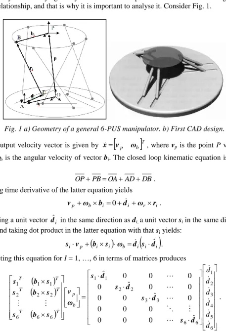
The inverse kinematics problem consists of obtaining the position/length of the actuators (also known as the configuration of the robot) given a desired position and orientation of the platform. For parallel manipulators, such as the 6-PUS robot, the difficulty to obtain the inverse and direct kinematics is inverted with respect to serial robots [10], [9]. Given a certain position and orientation p of the end effector, it is relatively simple to calculate the length of each articulation with a simple sum of vectors. Fig. 1 and equations 1 and 2 give an example of this. In Fig. 1, vector p represents the desired position of the end effector. Vector ai is a known parameter of the robot. The magnitude of vector bi is also a parameter of the robot, and its orientation is given by the desired orientation of the platform; di is the vector going from Ai to Di. By referencing all this vectors to the same coordinate system Ai, we can find the magnitude of each vector ri as ri=Aip + Aibi – Aiai – di. where p = [px py pz   ]T and the magnitude of ri represents the position/length of the actuator [9, 10]. Recall that , , and  are the Euler angles [10]. Working out the latter equation yields the closed form of the inverse kinematics for this manipulator:



 











}. , , { ; 6 ,..., 1 2 2 2 2 2 2 2 z y x j i r a b p a b p d i T i i i T i i ij ij j ij ij j ij                p b a p b a b a _{. (1)}

However, given the free nature of the universal and spherical joints, if the position/length of the actuators is known, it is not easy to calculate the platform’s position. Many researchers have studied the direct kinematics of the Stewart-Gough platform. Since the analytic solution requires solving a 16th degree equation, most of the articles that talk about this subject mention iterative numeric methods to solve the problem. It has been shown that because of the freedom possessed by the joints, given the length of the actuators it is possible to find 40 positions of the platform that satisfy equation (1) [3, 4, 10, 11]. Nevertheless, most of the studies refer to the 6-UPS platform, and very few [9, 10] analyse its variant 6-PUS. Compare with [14].

3.

Singularity Conditions

While kinematic analysis gives us a relationship between the position of the platform and the length of the actuators, sometimes it is important to know the relationship between the velocity of the actuated limbs and the angular velocity of the platform, especially while studying the dynamics of the manipulator. The Jacobian matrix gives us that relationship, and that is why it is important to analyse it. Consider Fig. 1.

Fig. 1 a) Geometry of a general 6-PUS manipulator. b) First CAD design.

The output velocity vector is given by x



v_p ω_b



T, where vp is the point P velocity and b is the angular velocity of vector bi. The closed loop kinematic equation is given by DB AD OA PB OP    . (2)

Taking time derivative of the latter equation yields

i r i i b p ω b d ω r v   0   . (3) Defining a unit vector dˆ_i in the same direction as di, a unit vector si in the same direction as ri and taking dot product in the latter equation with that si yields:



i i



b i

 

i i p

i v b s ω d s d

s       ˆ . (4) Rewriting this equation for I = 1, …, 6 in terms of matrices produces













                                                                6 5 4 3 2 1 6 6 3 3 2 2 1 1 6 6 6 2 2 2 1 1 1 ˆ 0 0 0 0 0 0 0 ˆ 0 0 0 0 ˆ 0 0 0 0 ˆ d d d d d d b p T T T T T T               d s d s d s d s ω v s b s s b s s b s . (5)

The latter equation implies that a parallel robot will present two kinds of singular configurations which will arise when the Jacobian matrices, shown in equation (6), become singular. Direct kinematics singularities come from det(Jx) = 0 and inverse kinematics singularities come from det(Jq) = 0.













                                      6 6 3 3 2 2 1 1 6 6 6 2 2 2 1 1 1 ˆ 0 0 0 0 0 0 0 ˆ 0 0 0 0 ˆ 0 0 0 0 ˆ , d s d s d s d s J s b s s b s s b s J         q T T T T T T x . (6)

An algorithm to compute numerically the constraints described above is given next.

Algorithm 1. Direct and Inverse Kinematics Singularities.

Step 1. Fix xmin, deltax, xmax; ymin,deltay,ymax; zmin,deltaz,zmax.

Step 2. For x=xmin:deltax:xmax. Step 3. For y=ymin:deltay:ymax.

Step 4. For z=zmin:deltaz:zmax.

Step 5. Compute vectors b according to the actual position b = f(x,y,z).

Step 6. Compute inverse kinematics d = f(x,y,z,b) with equation (1). Step 7. Determine vectors s for that position, s = f(d,x,y,z).

Step 8. Obtain Jx = f(b,s) with equation (6).

Step 9. Calculate and store |det(Jx)| for that point. Store these points in pJx. Step 10. Obtain Jq= f(d,s) with equation (6).

Step 11. Calculate and store |det(Jq)| for that point. Store these points in pJq. Step 12. End z, End y, End x.

Step 13. Plot the points pJx(x,y,z) obtained in step 9 in gradient colours. Step 14. Ídem for pJq(x,y,z) obtained in step 11.

The graphs and interpretations are given in section 8.

4.

Forward Kinematics: Numerical Algorithm.

As mentioned above, when we find the position and orientation of the platform given the position/length of the actuators, we are solving the direct or forward kinematics problem. The first thing that must be done is to establish the different coordinate systems that will be used: O is at the centre of the base, P at the centre of the platform, Ai at the beginning of each actuator, with the x axis pointing in the direction of the movement. Di and Bi are the ends of the ith leg, being Di the points that moves along the rail and Bi the point fixed on the platform. The method proposed in this paper assumes that the platform is a triangle in which there are only three connection points for the legs, one in each vertex, so that each point has two legs connected to it (see Fig. 2). This architecture is known as “6-3”. The general idea of the proposed method is that using the corresponding transformation matrices, three arcs corresponding to the possible locations of the three vertices of the triangle are generated.

So, the distances between each point of each arc and each point of the other arcs are calculated. After calculating all distances, we must find pairs of points whose distance is equal to the side of the triangle. See algorithm 1 which ends up with a numerical solution (section 8) of the direct kinematics for this proposed design [13].

Fig. 2 Modified design with triangular base and end effector.

Algorithm 2. Direct kinematics (method of arcs)

Step 1 Calculate the six transformation matrices oHAi [10],that transforms a coordinate

from system Ai to system O.

Step 2 Given the desired lengths of the actuators, find the points corresponding to the centre of the triangle formed by each pair of legs.

Step 3 For each of the three triangles, find its height and the angle rho between the axis of the two actuators.

Step 4 Find and plot all the points of that arc.

Step 5 Find, save and plot the distance between each point of arc 1 and each point of arc 2.

Step 6 Repeat last step using arcs 1 and 3, repeat last step using arcs 2 and 3.

Step 7 Find and save each pair of points (1, 2) whose distance is equal to the length of the platform’s.

Step 8 Repeat last step using arcs 1 and 3, repeat last step using arcs 2 and 3.

Step 9 Find the pairs of points (1, 3) whose point 1 exists on the list generated during step 8

Step 10 Find the pairs of points (2, 3) that exist on the list generated during step 11. Step 11 Save and plot the three points and the solution (platform).

5.

Inverse and Direct Dynamics

For the dynamic model, there are two different problems to solve. The direct dynamics derives the acceleration produced in the end effector, due to a given set of actuator forces. The inverse dynamics derives the forces needed in the actuators for a desired acceleration trajectory in the end effector. Little has been studied on the dynamics of parallel robots, and even less on that of the 6-PUS, [8-10, 12, 16]. In general, for parallel robots, the inverse dynamics is not very complex, but the direct dynamics is difficult to obtain due to possible existence of unknown reaction forces in the passive joints.

5.1 Inverse Dynamics

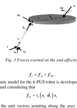
Consider Fig. 3. Let G be the platform’s centre of mass. The platform has a mass of m

and inertia matrix I. The acceleration of point G is denoted by aG. Let C be the point of application of external force Fand moment M. The force fiwhich acts on point Bican be decomposed on two components. The force fsi that goes along the main axis of the limb,

along unit vector si and the force perpendicular to si, due to inertia, which will be denoted fNi.

Fig. 3 Forces exerted on the end-effector.

We then have

Ni si

i f f

f   . (7)

In [9] a general dynamic model for the 6-PUS robot is developed, based on the dynamics of the 6-UPS model and considering that



ˆ



si τi i i i

f s d s (8)

where dˆ_iand si are the unit vectors pointing along the axes of the actuators and the limbs, respectively. However, this model does not consider the reaction forces exerted by the base and the actuators’ restrictions. The consequence of this omission is that every time the limbs are in a vertical position, the effect of the actuator forces on the platform becomes zero (note the dot product in the equation), and since these are the only forces considered in the model, the platform would fall down. To prove this, the model used in [9] was implemented in an algorithm which applies a constant force, and a simulation was run (see section of Numerical Simulations and [13], [10]). Now, in order to deduce the inverse dynamics of the robot we proceed as follows. First, we consider only the force exerted by the limbs on the platform according to (8). Let FN (3×1) be the resultant force of all fNi, i = 1, …, 6 and MN its resultant moment around point C. Let vector ci be the vector that goes from point C to point B. Let fsi = fsisi be the force that each limb exerts on the platform. The equations of equilibrium for the system are:

N i i si f s F F 



  6 1 , (9)





_N i i i si f c s M M



   6 1 . (10)

Let  and N the screw vectors for the external force and the resultant of the limbs, respectively. ) 1 6 ( ) 1 3 ( ) 1 3 ( ) 1 6 ( ) 1 3 ( ) 1 3 ( ,                       N N N _M F σ M F σ . (11)

Rewriting (9) and (10) in matrix form we have:                     



N N si i i i f M F s c s M F . (12)

We see that the first term of the right side of (12) is directly related with the Jacobian matrix Jx so that if we define a vector fs = [fs1,fs2,...,fs6]T we can rewrite equation (12) as:

N s T x f σ J σ  (13)

where fs is the 61 vector formed by the magnitude of each one of the forces that the limbs exert on the platform. Moment MG applied on the platform with respect to point G is

F e M

M_G    (14)

where e is the vector that goes from G to C; that is the moment arm of F. Let aG be the linear acceleration vector of point G. The Newton – Euler equations for the platform can be written as follows: G m mg a F  , (15) Iω ω ω I M_G    (16)

where g is the gravity acceleration vector and  is the angular velocity of the platform. Developing algebraically the latter equations and defining e* we obtain an expression for

, for any vector x, as follows:

 

                0 0 e -0 * is that , * 1 2 1 3 2 3 e e e e e e x e x e , (17) H W G σ   _{, (18)}

 

 





 



2 , * * * m m _m m m m         _{  }          e _{v g} G H ω Iω e v g e I e . (19)

These matrices have a physical meaning: G corresponds to the inertia matrix and H is the vector of forces due to gravity. By balancing (18) and (13) we have:

N s T x f σ J H W G     . (20)

With this we have derived the relation between the derivative of the twist over C (which corresponds to the acceleration) and the forces exerted on the platform by the limbs. Working out this equation we can find new expression for N, which in matrix form is expressed as: U W T σ    N , (21)

 

  

 

  

                             









    6 1 2 2 6 1 2 2 6 1 2 2 6 1 2 2 * * * , * * * i i i i i i i i i i i i i i i i i i i i i i r I r I r I r I L s c L s U K s c K s T . (22)

Substituting (22) in (21) yields and solving for fs, which corresponds to the forces that the limbs need to exert on the platform in order to generate certain acceleration W :



G T



W J



H U



J

f_s  _xT    _xT  . (23)

Each fsi points in the direction of the corresponding unit vector si. Neglecting friction on the universal and prismatic joints, Fig. 3 shows that this force fsisi is formed by three components: i Ni Ri i i i i f s  dˆ  kˆ nˆ . (24) where: . ˆ lar to perpendicu plane, xy on the vector , ˆ ˆ ˆ upwards. pointing r, unit vecto vertical ˆ i. actuator linear of direction in the r unit vecto ˆ n. restrictio s actuator' by the exerted force reaction vertical the of magnitude base. by the exerted force reaction vertical the of magnitude actuator. linear by the exerted force the of magnitude i i i i d d k n k d        Ni Ri i   

Note that dˆ_i,nˆ_i,kˆ are orthogonal and correspond to the x, y, and z directions of the coordinate system placed on A. For that reason, the three right-side members of equation (24) correspond to the x, y and z components of force fisi expressed on coordinate system

Ai. The rotation matrix Ai

RO can be derived from the construction parameters of the robot.             Ri Ni i i i O A si A f i i    s R f . (25)

Equations (23) and (25) then complete the inverse dynamics of the robot, with which we can solve the forces needed on the actuators (and the reaction forces of the base) for a desired acceleration trajectory.

5.2Direct Dynamics

The direct dynamics is more complicated. Even though it is simple to solve (23) and get an expression of the acceleration in terms of the forces exerted by the limbs (equation 26), as seen before such forces are made up of three components, of which only one is known.



G T



J f



G T

 

H U



W   1 _xT _s  1  . (26) Just as the inverse kinematics is relatively simple for parallel robots, but direct kinematics is complex because we do not know the values of the passive joints, we can see that the direct dynamics in this case is made difficult due to the lack of information of the reaction forces. We know, however, that these forces exerted on point D produce no work since there is no displacement in those directions. The Virtual Work Principle tells us that we can write an equation using the differential displacements of each of the

points in the mechanism, due to the forces applied on each point, and the total sum of the work produced by each force in that case is zero. In other words, assuming that the forces on the platform oppose and cancel the forces on the actuators, we then have that for differential (translational and rotational) displacements  x = [ P  ]T, the total work produced is [10, 15]: 0         _{  } _     τ d F P M Θ . (27)

We can use Jacobian matrices to relate the differential displacements on the platform to differential displacements on the actuators.

x



 q



J x J d, (28)

xJ d . (29)

Substituting (28) in (26) and after some algebraic development we obtain in (30) the direct dynamics model of the robot

H G τ J G W  1 T  1 . (30)

6.

Kinematic Control

As mentioned in section 2, the inverse kinematics of this 6-PUS manipulator is given by equation (1). So, given a desired position p, the result will be an actuator vector d = [d1…d6]T which says how long each actuator must expand or contract to achieve the desired position d. It is easy to see that in order to generate a desired trajectory, a set of positions p is required. As a consequence, a kinematic position control (open loop) can be done by programming equation (1). The corresponding experiments were done and are given in section 8.

7.

Dynamic Control

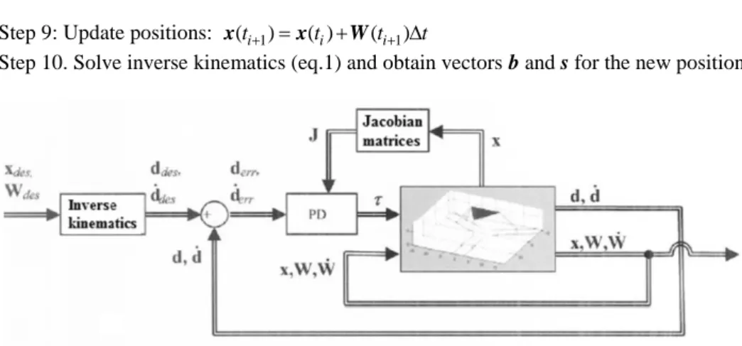
Equation (30) had to be constructed on line during numerical simulations in order to implement a closed loop system with a PD controller (Fig. 4). The block with a little robot image represents such equation (30). As a consequence of the symmetric architecture of the robot, we chose matrices Kp = kpI and KD = kdI, kp, kd+, with I the identity matrix of order six, see Fig. 3. Section 8 provides results.

Algorithm 3. PD controller.

Step 1 Fix position, velocity and acceleration initial conditions.

Step 2 Solve inverse kinematics with algorithm 1 and obtain vectors b and s. Step 3. Fix t_initial, t, t_final; While t  t_final do step 5 to step 9.

Step 4. Choose the desired d as d_des, obtain Jacobian matrices and error vectors d_err,

_err d .

Step 5. Compute matrices T, U and G, H solving equations (19) and (22), respectively. Step 6. Compute τK d_{p err}K d_{D err}

.

Step 7. Determine accelerations in terms of force with equation (30). Step 8. Update velocities: W(t_i1)W( )t_i W( )t_i t

Step 9: Update positions: x(t_i1)x( )t_i W(t_i1)t

Step 10. Solve inverse kinematics (eq.1) and obtain vectors b and s for the new position.

Fig. 4 Complete closed loop control system for the 6-PUS parallel robot.

8.

Numerical Simulations

In this section, we provide the simulations corresponding to the inverse and direct kinematics cases, direct and inverse dynamics problems as well as kinematic and dynamic control.

8.1 Inverse Kinematics.

This case is illustrated with two examples. The first one considers a fixed desired position given by p = [px py pz   ]T = [–1 3 5 0.2 0.3 –0.8]T. The resulting actuator vector d yielded to be d = [5.49 4.96 1.87 2.15 5.09 5.57]. The second example resulted to be more interesting. A desired trajectory is stored in a long vector p in order to write down a letter “M”. See Fig. 5.

Fig. 5 Writing down letter “M” needs these trajectories of the six actuators.

8.2 Inverse Kinematics Singularities.

Matrix Jq has full rank within a region close to the origin of the workspace. So, for any given point in the workspace, as longer the distance from the origin, as closer Jq to loose rank. The following figure illustrates the values of |det(Jq)| in the workspace.

Fig. 6 Values of |det(Jq)|.

It is possible to plot a surface associated to the latter figure where det(Jq) = 0. This surface represents the workspace of the manipulator. See Fig. 7.

Fig. 7 Surface where det(Jq) = 0. 8.3 Direct Kinematics

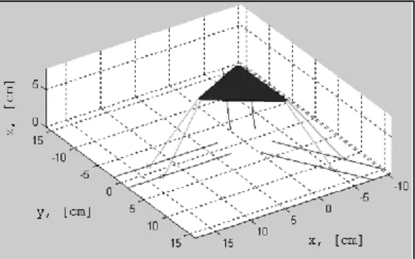
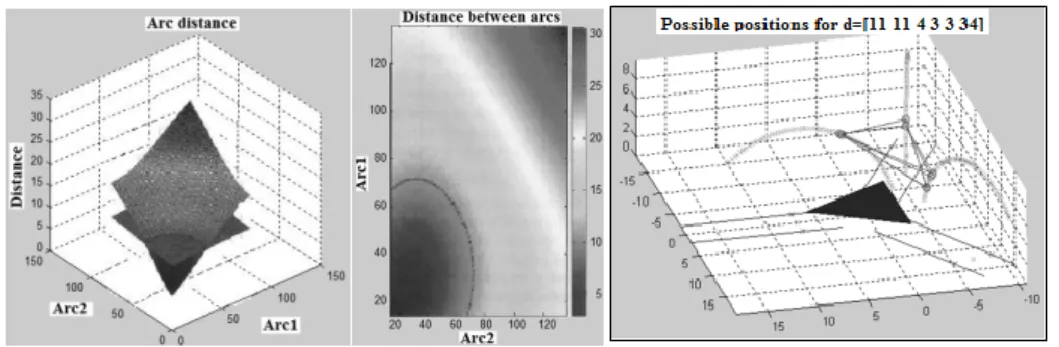
The results for the direct kinematics are presented here. Fig. 8a shows the arcs generated by each pair of legs. The distance between each pair of points of arcs 1 and 2 is also shown. The horizontal plane corresponds to the length of the side of the platform and the crosses represent the pair of points whose distance is equal to the same one as the side of the platform. The white dot is the final solution found by algorithm 1 (Section 3). Fig. 8b shows the base of the manipulator along with the rails of the actuators. Here three resulting positions of the platform are shown for a given actuators vector d [13].

Fig. 8 a) Distance between points belonging to arcs 1 and 2.

b) Resultant positions of the platform.

In [2] there is a very general methodology to obtain the direct kinematics of any parallel robot using an iterative algorithm. That algorithm was implemented for the robot analysed in this paper; however, the geometric method proposed in this paper –inspired by a solution presented by [1] gave better results than those obtained by the iterative method based on the work presented in [2]. It is important to note that the method works because the configuration 6-3 simplifies each pair of legs, as one leg with only one degree of freedom. This is a very useful technique when working with parallel manipulators. We can also see that in this type of manipulators it is very common for the direct kinematics to have many solutions, so in order to plan a trajectory it is very important to know the previous position.

8.4 Direct Kinematics Singularities.

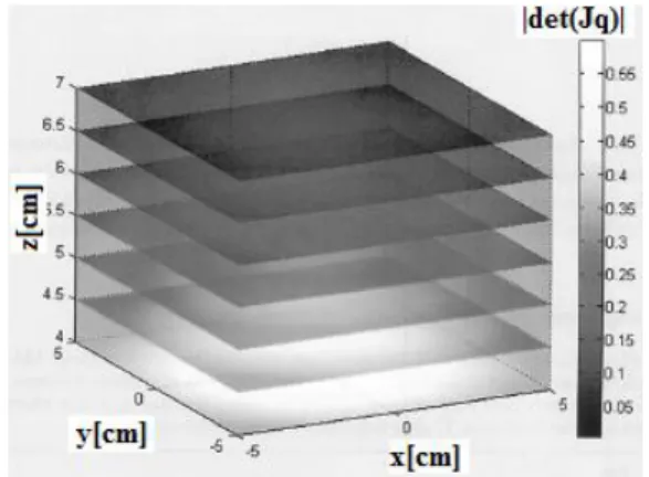
Proceeding in this case, as it was done for the inverse kinematic singularities, a figure is obtained which shows |det(Jx)|.

Fig. 9 Numerical values of |det(Jx)| in the workspace

Darker regions appear as closer to the centre of the workspace we are. This means that Jx loses rank when the platform is close to the base. This happens when limbs and motion axes are collinear. Observing Fig. 9, it is deduced that x, y, and z should be limited to

the platform within some fixed values like those, it is important to determine what position corresponds to the actuators parameters. This issue is solved by the direct kinematics.

8.5 Inverse Dynamics

As it was explained in Section 5.1, the reaction forces exerted by the robot’s base and actuator’s restrictions were not taken into account in [9]. Hence, when the robot is standing up (completely vertical position), it falls down. To illustrate this fact, the model considered in [9] was implemented in an algorithm which applies a constant input force. Simulations revealed the resultant behaviour just described. Acceleration and position trajectories described that every time the vectors s are in a vertical position, the actuator forces have no effect on the platform, and thus it falls down. As it does, s vectors start losing verticality, since the dot product (sd) rises, and the actuator forces have an effect on the platform and it rises again. In order to improve the model, the reaction forces of the actuator restrictions were taken into account. See plots in [16].

8.6 Direct or Forward Dynamics

Since forward dynamics is needed to solve the control problem (see Dynamic Control Section), the simulations for open loop forward dynamics were omitted but see [16].

8.7 Kinematic Control Simulations and Models proposed

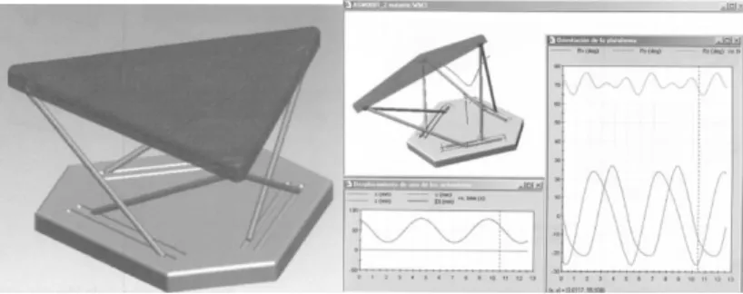
It was explained in Section 6 (Kinematic Control) that an open loop position control can be numerically implemented by programming equation (1), i.e. the inverse kinematics vector equation. With all the background developed so far, it was possible to create several animated 3D designs in Visual Nastran. Two of them are shown in Fig. 10. After refining the whole modelling and control design, a triangle shape was chosen for the base and end effector. See also Section 4.

Fig. 10 Early stage 3D render model designs.

8.8 Dynamic Control.

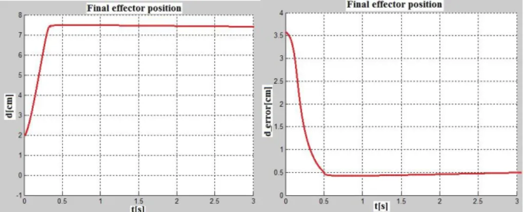
The control loop was designed to have a good regulation performance. Laser cuttings are done via series of step inputs. A simple PD controller was proposed to control the robot’s platform in the joint space for each actuator. Since the robot presents a symmetric architecture, all the controllers were chosen identical. The results of the PD controller performance are described next for a step input of amplitude 7cm. The platform position in “z” (platform height) behaved as is indicated in Figs 11a and 11b.

The resulting steady state error in the actuators was 0.5cm, about 7% of the final value. The controller gains were kp = 300 and kd = 30.

Fig. 11 a) PD controller step response of the platform . b) Steady state error.

In order to improve the latter performance, a PD plus gravity compensation (PD+G) was also implemented. So, step 6 in algorithm 3 was replaced by the following command: Step 6: Compute





T 0 0 0 mg 0 0 T err D err pd K d J K τ   

In this case the steady state error was equal to zero after 0.75 seconds of raising time.

Fig. 12 a)PD+G controller step response b) Steady state response.

8.9 Laser Cutting Machine application design

As it is well known and as it was mentioned in the Abstract and Introduction, parallel robots have a higher payload than their serial counterparts. Mounting a laser cutting device under the robot platform would not modify all the mathematical modelling developed until now. The inertia terms do not change a lot as a result of the inherent light weight of the laser device, as well as the above mentioned payload. For instance, consider to cut a piece following an “M” shape as illustrated in Fig. 13. If such a task is developed with kinematics (see Fig. 5) or by dynamical control (see Fig. 12) the goal will be accomplished. Since the robot architecture is symmetric, the actuators and the PD+G controllers are identical among them. As a consequence, the cutting process will succeed as deduced from the initial design until the closed loop control.

Fig.13 Parallel robot-based laser cutting machine numerical prototype.

9.

Conclusions

In this paper, a novel design of a 6-PUS parallel robot was given. Besides, a new method to solve the forward kinematics was presented. In addition, inverse and forward dynamics problems were solved in order to implement a control system for the inverse dynamics model. Singularities were found numerically and a PD and a PD+G controllers were designed for this robot. Both controllers presented a good performance, although PD+G’s was definitely better. The controllers’ performance was good enough for the present purposes and as a result of their relative simplicity it was not necessary to deal with numerical problems as stiffness, convergence, algebraic loops, etc., as with nonlinear/intelligent controllers. High payload and PDs help to deal with varying inertias on the platform or below it as a laser cutter device.

References

[1] ÁNGELES, J. Fund. Rob.Mech.Systems. New York: Springer, USA, 2003, 254 p. [2] BRUYNINCKX, H. Parallel Robots. The Robotics WEBook. [on line], August

2005.<https://static.aminer.org/pdf/PDF/000/351/256/dualities_between_serial_and _parallel_manipulators.pdf>.

[3] CRUZ, P. and FERREIRA R, Kinematic Modeling of Stewart-Gough Platforms. In

ICINCO 2005 Rob. Autom. Barcelona: Spain, Springer, 2006, p. 93-99.

[4] GAO, X; et al. Generalized Stewart-Gough Platforms and Their Direct Kinematics.

IEEE Trans. on Robotics, 2005, vol. 21, no. 2, p. 141-151.

[5] HOPKINS, B. and WILLIAMS R. Kinematics, design and control of the 6-PSU platform. The Industrial Robot. Bedford, 2002, vol. 29, no. 5, p. 443-445.

[6] JAFARI, F. and MCINROY, J. Orthogonal Gough-Stewart Platforms for Micromanipulation. IEEE Trans. on Rob. Autom., 2003, vol.19, no.4,p.595-603. [7] KHALIL, W. and GUEGAN, S. Inverse and Direct Dynamic Modeling of

Gough-Stewart Robots. IEEE Trans. on Rob., 2004, vol. 20, no. 4, p. 754-762.

[8] LING-FU, K. and SHI-HUI, Z. Research on a Novel Parallel Engraving Machine and its Key Technologies. Int. J. of A. Rob. Syst, 2004, vol. 1, no., 4, p. 273–286. [9] MERLET, J. Parallel Robots. Dordrecht: Springer, 2006, 412 p.

[10] TSAI, L. Robot Analysis. New York: Wiley, 1999. 520 p.

[12] YIU, Y. K. and H. CHENG. On the Dynamics of Parallel Manipulators. In Proc. of the 2001 IEEE Int. Conf. Rob. & Aut. Seoul: Korea, IEEE, 2001, p. 3766-3771. [13] RUIZ-GARCÍA, J. and ZAVALA-YOÉ, R. and CHAPARRO-ALTAMIRANO, D.

and RAMIREZ-MENDOZA, R. Direct Kinematics of a 6-PUS Parallel Robot Using a Numeric-Geometric Method, In Proc. of the IEEE Int. Conf. Mech., Elec. Auto. Eng. Morelos: México, IEEE, 2013, p. 46-50.

[14] CHAPARRO, D. and ZAVALA-YOE, R. and RAMIREZ-MENDOZA, R. Kinematic and Workspace Analysis of a Parallel Robot Used in Security Applications, In Proc. of the IEEE Int. Conf. Mech. Elec. Auto. Eng., Morelos: México, IEEE, 2013, p. 3-8.

[15] HIBBELER, R. C. Eng. Mech. New Jersey: Prentice Hall, 1998, 315 p.

[16] RUIZ-GARCÍA, J., ZAVALA-YOÉ, R. CHAPARRO-ALTAMIRANO, D., RAMIREZ-MENDOZA, R. Direct and Inverse Dynamics of a 6-PUS Parallel Robot, In Proc. IEEE Int. Conf .Mech. Elec. Auto. Eng. Morelos: México, IEEE, 2013, p. 21-26.