Performance evaluation of packet capturing systems for high-speed networks

(1)

Technische Universit¨

at M¨

unchen

Fakult¨

at f¨

ur Informatik

Diplomarbeit

Performance evaluation of packet

capturing systems for high-speed

networks

Fabian Schneider

Aufgabenstellerin: Prof. Anja Feldmann, Ph. D. Betreuer: Dipl.-Inf. J¨org Wallerich Abgabedatum: 15. November 2005

(2)

(3)

Ich versichere, dass ich diese Diplomarbeit selbst¨andig verfasst und nur die angegebe-nen Quellen und Hilfsmittel verwendet habe.

(4)

(5)

Abstract

Packet capturing in contemporary high-speed networks like Giga-bit Ethernet is a challenging task when using commodity hard-ware. This holds especially for applications where full packets (headers and data) are needed and packet loss is unwanted. Most network security tools—particularly network intrusion detection systems—have these demands.

Therefore, it is interesting to know if todays customary hardware and software are able to keep up with the network in terms of throughput of packet data. A methodology for evaluating the performance of different systems for packet capture is described and applied in this thesis. Four different PC based systems are compared with respect to their maximum capturing rate.

As modern PC’s are available with different types of processor ar-chitectures which can then be equipped with different operating systems, it is interesting to find out which combination performs best for the task of packet capturing. The measurements per-formed for this thesis evaluate Intel Xeon against AMD Opteron based systems running either Linux or FreeBSD.

For this purpose, the Linux Kernel Packet Generator has been extended by the feature to not only generate packets of a given size, but to generate packets according to an underlying packet size distribution. This workload source provides all four systems with high bandwidth traffic which has to be captured.

The results show that the combination of AMD Opterons with FreeBSD outperforms all others, independently of running in sin-gle or multi processor mode. Moreover, the impacts of packet fil-tering, using multiple capturing applications, adding packet based load, writing the captured packets to disk, and available enhance-ments are measured and looked into.

(6)

(7)

Contents I/II

1 Introduction

Packet capturing is the process of reading the transfered data units from a network link1. When capturing on an Ethernet2 link, one reads these whole data units, called frames, except for the preamble and the checksum which are stripped off by the network card. Because there are different protocol implementations for the data link layer3, and because the more interesting part of the captured data is inside the encapsulated network layer3 _{part of the frame, the term “packet” will be used for}

an Ethernet frame, an IP packet, or a transport protocol3 _{data unit. Furthermore,}

the term “packet capturing” refers to this “relaxed” meaning of “packet”.

1.1 Motivation

Packet capturing, or sniffing4, is the instrument used most often for network secu-rity tools, such as intrusion detection or prevention systems, and network analysis tools. In either case it is important to capture all the packets transfered over the link. This holds especially for application layer protocol analysis which requires the complete stream of packets of the examined connection. One could argue that of-ten the necessary information needed for the analysis can already be found in the first few packets of a connection and thus loosing packets (later on) does not hurt. But the opposite is the case: If only few packets per connection are required, it is exceptionally bad if exactly these packets are lost. Altogether, no packet should get lost.

Therefore, it is interesting to know if the system is able to keep up with the amount of data or with the arrival rate of the single packets. Usually, in a Fast-Ethernet2 environment this is no problem for most of todays hard- and software. But looking at Gigabit-Ethernet2_{, todays limits in terms of PCI bus}5_{throughput, CPU capabilities,}

storage speed, or application (resource) demands can easily be exceeded. And with the next step to 10-Gigabit-Ethernet2 in mind, it is necessary to understand the complexity of packet capturing.

1

Link refers to a physical connection between network devices. In addition all attached devices are required to be ready for sending and receiving data for calling this connection a link.

2

For protocol details ofEthernetplease see [Tan03, Section 4.3, pages 271 et seqq.].

3

Theselayersare part of the ISO/OSI reference model. See [Tan03, Section 1.4.1, p. 37 et seqq.].

4

Sniffingis a more informal word and often bears a negative or illegal meaning. The term “sniffers”

will be used for the machines performing packet capture.

5

A PCI busis used to connect peripheral components to the mainboard of a contemporary PC.

Besides the slot itself the protocol and the speed of the bus is defined by PCI. Meanwhile different variants of PCI are available: PCI-X or PCIexpress are the newest among them.

(10)

The intended purpose of this thesis is to compare computers in multiple config-urations while capturing packets. Thereby, many performance influencing factors are evaluated in order to gain more insight in the complex topic of packet captur-ing. The interpretation of the results of this comparison shall enable the reader to choose an appropriate system for his or her special task. The measurements for this comparison are all done with respect to the percentage of the captured packets in relation to the total available packets. This ratio is a metric for the packet capturing performance of the system.

The major factors influencing the performance of packet capturing, physical system throughput, and the delay and the amount of work between receiving the packet and delivering it to the application, are quite obvious. For the purpose of this thesis, it is necessary to supply the possibility to compare different flavors of these factors. On the one hand, two different architectures affecting the throughput were purchased: dual Intel Xeon and dual AMD Opteron machines. One of the fastest network cards and a system bus capable of at least 1 Gbit/s of continuous bandwidth were chosen. On the other hand, different operating systems supply different means and mechanisms to provide applications with raw network data. Thus, FreeBSD and Linux, the most popular operating systems for the task of capturing packets, are examined.

1.2 Related Work

The project thesis [Sch04] describes similar work on single-processor systems per-formed last year. The following paragraphs will give a brief summary of that work consisting of two main parts.

The first part was an analysis of the “capturing stacks” of Linux and FreeBSD. The mechanism used to capture packets is called capturing stack in analogy to the network stack which is used to receive and send packets and which is located in the kernel as well. The purpose was to identify the differences between Linux and FreeBSD, two readily available Open Source operating systems. A source-code investigation of the kernel and the libpcap [JLM94] (see Section 2.1.3) turned out that during the processing of a packet Linux copies the data two times whereas FreeBSD copies it three times, thus giving an advantage to Linux. On the other hand it is necessary to do reference counting to keep track of the packet data stored in the kernel memory. On that account the Linux kernel has to deal with big buffers that—in worst case—do not deplete.

The one additional copy which FreeBSD performs is due to a double buffer strategy used by the kernel built-in filter from which the application can read the packets. In contrast Linux stores the packets in an area of kernel memory reserved for incoming packets. The double buffer of FreeBSD is replaced by a queue of pointers. This leads to another difference: Under FreeBSD the whole content of one half of the

(11)

1.3 Structure of this Thesis 3/86

double buffer is copied into the user space, whereas Linux performs a separate copy operation for every single packet. The general principle of packet capturing with Linux and FreeBSD is explained briefly in Section 2.1.

The second part of the project was a comparison measurement of Linux and FreeBSD. It was not possible to generate test packets at line speed—so that the maximum throughput of the link is fully utilized—with the available hardware. Hence, only data rates between 150 MBit/s with minimal small packets (40 Bytes) and about 500 Mbit/s with maximum large packets (1500 Bytes) could be achieved.

With only one capture application, Linux performed better than FreeBSD. But with multiple concurrent capturing applications, FreeBSD shares resources more evenly between the applications than Linux does. In this case all applications obtain nearly the same number of packets with a deviation of about five percent under FreeBSD. Under Linux it happens that one application only sees about five percent and another application captures nearly all of the generated packets. Comparing the average capturing rates yields that this time Linux is inferior. Together with the findings from the first part, this shows that different operating systems cause different capturing performance.

Further results show that different network cards with their corresponding drivers just as buffer settings have a great influence on the loss ratio. For precise results please take a look at [Sch04].

In addition, Luca Deri [Der04, Der03] has to be mentioned who worked on improv-ing the packet capturimprov-ing abilities of Linux usimprov-ing a rimprov-ing buffer design. He also did measurements on this topic. The performance of his patch was also subject to the project work described above.

1.3 Structure of this Thesis

In the next section (2.1) the principal procedure of packet capturing for Linux and FreeBSD is outlined as well as the most important procedures of the libpcap, a common library used for packet capturing. The difficulties of packet capturing— throughput, copy operations, and receive livelock—are discussed in Section 2.2. Sub-sequently, Section 2.3 presents our regular environment and applications of the sys-tems under test. Because this thesis compares syssys-tems equipped with Intel Xeon and AMD Opteron processors, the differences of these architecture designs are pointed out in Section 2.4. A short summary of network traffic characteristics in Section 2.5 ends Chapter 2.

Chapter 3 introduces the methodology underlying the measurements. Section 3.2 first identifies the requirements on the hard- and software participating in the ex-periments. The test setup is shown in Section 3.3, and the measurement cycle is illustrated in Section 3.4.

(12)

Chapter 4 begins with the identification of the capabilities of existing tools for packet generation with respect to the intended measurements in Section 4.1. Because none of these tools meets the requirements stated in the previous chapter, the following sections describe how the Linux Kernel Packet Generator was improved. How to ac-quire suitable packet size distributions is explained in Section 4.2. The performance of this enhanced Linux Kernel Packet Generator is tested in Section 4.3.

Chapter 5 defines the form of profiling used to monitor the CPU usage of the systems under test.

Before the results of the measurements are shown in Chapter 6 the factors influencing the capturing process are itemized in Section 6.1. The parameters of the used methodology are specified in Section 6.2 and the results are stated in Section 6.3. Chapter 7 summarizes the results and motivates further work.

A short guide to the programs written for this thesis is given in Appendix A. Supple-mental plots of further results (Appendix B), and acknowledgements (Appendix C) complete this thesis.

(13)

5/86

2 Background

As this thesis aims at identifying benefits and drawbacks for packet capturing, differ-ent scenarios have to be evaluated. To understand which settings and circumstances affect the process of packet capturing, the process itself has to be apprehended. Fur-thermore, the surroundings of packet capturing have to be spotted. This chapter intends to provide the background for the remainder of this thesis.

2.1 How does Packet Capturing Work?

Before delving into the used environment and problems arising when capturing pack-ets, this section explains how the capturing is done in general. But since every operating system has its own functionalities to actually perform the capturing and the filtering, this cannot be done quick and easy. Therefore, only the researched operating systems FreeBSD and Linux are elucidated. Please refer to [Sch04] for a detailed description. The research of further operating systems, such as Windows, MacOS or Solaris, would go beyond the scope of this thesis. But the equivalent mechanisms for capturing packets exist for these operating systems as well.

2.1.1 Capturing with FreeBSD – the BSD Packet Filter

The BSD Packet Filter (BPF) was introduced in 1992 by Steven McCanne and Van Jacobson [MJ93] as a packet filter for BSD. The main advantage of this at that time new design is to be able to filter the packets before they are copied to the user space1_{, thus saving an expensive copy operation if packets are rejected by the filter.}

Another improvement is the new filter description language which is comparable to assembler. The benefit of this new language is that, instead of using a boolean decision tree, it uses a control flow graph, which allows shortcuts and smart filter programs. The filter is implemented as an independent machine within the kernel code. Figure 2.1 demonstrates the design of the BPF.

When packets arrive at a network card the card verifies the checksum, extracts the link-layer data, and triggers an interrupt2. This interrupt calls the corresponding

1

In contrast to kernel space the user space is the segment of the memory of a system which is available to the applications. In opposite device drivers and kernel stuff is stored in kernel space.

2

Aninterruptis used to suspend the normal processor operation for special events. These events

concern peripheral devices such as disks, or—in this case—network interface cards. In general, an interrupt signals the processor that data is ready to fetch. For further information on interrupts and their processing please refer to [Tan01, Sections 1.4.3 and 5.1.5, pages 30 and 279 et seqq.].

(14)

kernel driver kernel driver kernel driver BPF network stack HOLD Buffer STORE Buffer HOLD Buffer STORE Buffer filter filter network kernel kernel user ... network cards rarp USER Buffer libpcap Library libpcap calls User code browser double buffers

Figure 2.1: Block diagram of the BPF: This figure shows the general concept of the BSD

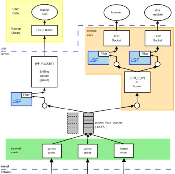
Packet Filter. kernel driver kernel driver kernel driver network kernel kernel user network cards USER Buffer libpcap Library libpcap calls User code packet_input_queues ( 1/CPU ) (ETH_P_IP) IP Socket (PF_PACKET) Sniffing Socket (queue) LSF Filter UDP Socket TCP Socket LSF Filter LSF Filter browser dns resolver network stack

Figure 2.2: Block diagram of the LSF: This figure shows the general concept of the Linux

(15)

2.1 How does Packet Capturing Work? 7/86

kernel driver for the card which generates the kernel structure for network packets. This is like adding a handle for the operating system to the packet. Then the kernel passes the packet to every BPF in use (one for each application which is capturing) and to the normal network stack. Still in the interrupt handler, the previously installed filter is applied, and if the packet is accepted it is copied into the STORE half of the double buffer. Now the captured data can be fetched through a read on the /dev/bpf[0-9]+device from the HOLD buffer. These buffers are switched if either the STORE buffer is full and a packet is waiting, or if the HOLD buffer is empty and the application performs a read. A more convenient way of accessing the data through the BPF is to use the interfaces supplied by the libpcap (see Section 2.1.3) which was developed in parallel to BPF.

2.1.2 Capturing with Linux – the Linux Socket Filter

The Linux Socket Filter (LSF) is a slightly extended BPF. The only conceptual difference is the ability to use it at divers positions in the network stack in addition (see [Ins01, Ins02a, Ins02b] for details). The internal handling of packets within the Linux kernel is performed via so called “sockets”. These “sockets” have nothing in common with sockets known from UNIX, which are used to access the network from user space. A “socket” in the current context is a smart queue for pointers to packets stored by the kernel. Each “socket” is in charge for a class of packets. For exampleETH P IPknows what to do with IP packets within the network stack. In contrast to FreeBSD, the interrupt spawned by the network card only puts a pointer to the packet into a queue and schedules a soft-interrupt3_{. This soft-interrupt}

hands the packets over to every “socket” which fits to the given packet (see Fig-ure 2.2). Thus, a “socket” matching any packet (PF PACKET) is needed. As it is possible to bind an LSF on any “socket”, this concept is comparable to BPF, es-pecially when considering that the filter description language is the one from BPF. The packets accepted by the attached LSF are queued. If no filter is attached, all packets are queued. If there are packets available, the applications registered for that socket are woken up to fetch the data. Contrary to FreeBSD, the packets are copied separately to the user space whereas FreeBSD copies the whole buffer at once.

2.1.3 libpcap – the packet capturing library

As previously mentioned, the libpcap [JLM94] is a C library for capturing packets. The procedures included in libpcap provide a standardized interface to all common (UNIX-based) operating systems, including Linux and FreeBSD. The interface of

3

Unlike a (hardware) interrupt which is originated from some kind of attached hardware, a

soft-interrupt is generated by the kernel to remind itself to do something. Soft-interrupts do no

(16)

the libpcap is usable even under Windows but there the library is called winpcap. So it is useful to design applications to use libpcap for ensuring portability.

The most popular tool for quick network monitoring and network debugging is tcp-dump (www.tcpdump.org). Nowadays libpcap is developed in parallel with tcp-dump.

Among others, these are the most important procedures of libpcap:

pcap open live() opens a new “capturing session” which is represented by astruct

of type pcap. This structis necessary for any further processing in the ses-sion.

pcap next() sets a pointer to the next packet.

pcap loop() binds a user defined function for packet data processing to a pcap

struct. This function is called for every captured packet. This procedure can be used instead of pcap next().

pcap setfilter() can be used to install a previously (withpcap compile()) com-piled filter to the “capturing session”. When supported (as under Linux and FreeBSD), the filtering mechanisms of the kernel are used for this.

Further procedures deal with writing captured packets to a file, reading and rewriting these files, with management of the “capturing session”, and statistics processing. For a detailed description of the procedures please refer to the manpage of libpcap (man pcap).

2.2 General Problems while Packet Capturing

This sections addresses the problems most relevant for packet capturing.

2.2.1 Receive Interrupt Load

As every received packet generates one interrupt, at high packet rates the incoming packets produce such a high interrupt load that the packet processing application does not get enough computing cycles to do its work or read the packets from the filter. This leads to full buffers and massive packet drops. In [MR97] the authors describe this problem called receive livelock in detail. To avoid receive livelock, Mogul and Ramakrishnan proposed the following solutions:

• Using polling in overload situations to limit the interrupt arrival rate and re-turning to use interrupts afterwards. Instead of generating one interrupt per packet the operating system frequently polls the network card for new packets, thus conserving resources for packet processing. More information on device

(17)

2.2 General Problems while Packet Capturing 9/86

polling can be found in [SOK01, for Linux (NAPI)], [Riz01, for FreeBSD], [RD01, for Windows] and [Der04].

Another way of reducing the interrupt load is to do interrupt moderation which actually is nothing else than gathering some interrupts before originating one. This approach is available with the up-to-date Intel and Syskonnect Network Cards.

The disadvantage of both device polling and interrupt moderation is that the timestamping of the packets which is usually performed by the receiving inter-rupt in the kernel assigns the same timestamp to multiple packets. Thereby, the packet order might be falsely interpreted by the analyzing application. In any case, the timestamps of most packets and along with this the inter-packet gaps are not correct. To counter this problem, some network cards are able to timestamp the packets themselves.

• Processing received packets to completion to avoid buffering packets which are overwritten later by others or dropped because of full queues. This ensures that even under excessive load the packets that were captured are useful.

• Explicitly regulating the CPU usage for packet processing to grant more process-ing time. This can be achieved using systems trimmed for real-time operation (see [AGK+_{02, GAK}+_{02, Kuh04]). This helps granting the kernel a unique}

utilization of the resources and therefore leads to better performance.

2.2.2 Packet Copy Operations

As described in Section 2.1, packet data is copied multiple times until it arrives at the application in user space. Copying packets within the kernel is expensive in terms of CPU cycles. Thus, reducing the number of copy operations improves the capturing capabilities.

In the FreeBSD capturing stack, the packet is copied three times:

• The first time from the network card to the main memory,

• then into the double-buffer behind the filtering engine,

• and finally from this buffer to the user space application. There are several approaches to reduce these copy operations:

Linux avoids the second copy because there is no buffer behind the filtering engine. Instead, Packet data is located via a pointer in the queue behind the filter and delivered to user land.

(18)

Memory-mapped buffers can be used instead of the double-buffers or the kernel memory where the packets are kept. The principle of memory-mapping is to allow access from kernel as well as from user space to some piece of memory. When used as buffer, the access to this memory has to be shared. Therefore, they are often implemented as ring-buffers. This reduces the number of copies by one.

The measurements of Luca Deri for testing his ring buffer patch on the “capturing stack” of Linux [Der04, Der03] were only done on a single processor machine. Our experience is that this ring-buffer patch does not work stable with a multiprocessor kernel. Therefore, this patch will not be considered in this thesis.

2.2.3 I/O Throughput

When writing captured data to disk or when displaying per-packet information on a terminal which is probably accessed via some kind of remote login, a further performance bottleneck is added. As one can never capture more packets than the harddisk can write, it is crucial to consider this bottleneck. For example, terminals have a maximum printing rate which is easily exceeded with the bandwidth of a fully loaded Ethernet.

As experience has shown, even the PCI bus can be the bottleneck in a fully utilized Gigabit Ethernet environment, even though the theoretical maximum throughput suffices. Hence, it is necessary to use PCI enhancements like PCI-64bit, PCI-X, or PCIexpress in such situations.

2.3 Environment

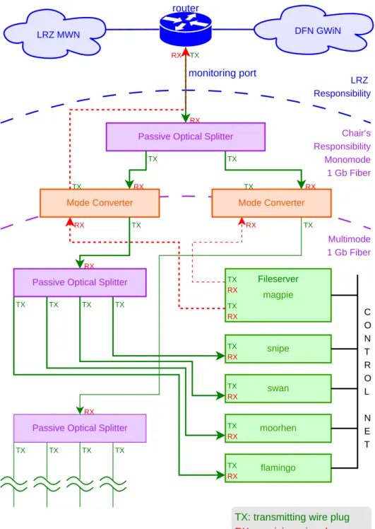
As mentioned before, different machines are to be examined. One reason to purchase them was to evaluate their performance regarding packet capturing, as done in this thesis. Another reason was the intended purpose of these machines. In production deployment, the four double-processor computers are arranged for traffic capture at the edge of the scientific network of Munich (MWN) (see Section 4.1.4 for details). snipe,swan,moorhenandflamingoare the machines used for capturing. The captured data can then be used for traffic analysis. Another objective of these systems in regular operations is further development of intrusion detection systems. Thus, “production” is used in terms of academia here, mainly for research. The table in Figure 2.4 shows the differences between the machines.

All sniffers are equipped with 2 GBytes of RAM, an Intel 82544EI Gigabit (Fiber) Ethernet Controller, and a 3ware Inc. 7000 series ATA-100 Storage RAID-Controller with at least 450 GBytes of harddisk space attached. The Intel Xeon architecture machines are capable of Hyperthreading (see Section 6.3.7 for details).

(19)

2.3 Environment 11/86 flamingo DFN GWiN LRZ MWN monitoring port LRZ Responsibility Chair’s Responsibility

Passive Optical Splitter

snipe moorhen magpie swan Multimode 1 Gb Fiber Passive Optical Splitter

Monomode 1 Gb Fiber

Passive Optical Splitter

Mode Converter Mode Converter

TX TX TX TX TX RX RX RX RX RX RX TX TX TX RX RX TX RX RX TX TX RX TX TX TX TX TX TX TX TX TX RX RX router

TX: transmitting wire plug

RX: receiving wire plug

C O N T R O L N E T Fileserver TX RX

Figure 2.3:Network diagram of the regular setup of the capturing machines: The capturing

interfaces of the different sniffers are attached to an optical splitter which distributes the input from a monitoring port at the uplink router of the LRZ.

(20)

Figure 2.4: The diversity of the sniffers.

Name Architecture (Cache) Chipset OS

swan AMD Opteron 244 (1024 kB) AMD 8111 Linux 2.6.11.x moorhen AMD Opteron 244 (1024 kB) AMD 8111 FreeBSD 5.4 flamingo Intel Xeon 3.06GHz (512 kB) SW GC-LE/CSB6 FreeBSD 5.4 snipe Intel Xeon 3.06GHz (512 kB) SW GC-LE/CSB6 Linux 2.6.11.x

Figure 2.3 demonstrates the regular setup opposed to the measurement setup for this thesis explained in Section 3.3. The network traffic obtained from the moni-toring port at the edge router has to be duplicated several times. For that purpose optical splitters are used because their only influence is a reduced signal strength. This seems to be no problem, at least with the short cables that are used in this environment. Since there are no intelligent circuits or even electronic parts used as in a switch, the problem of timing issues, packet drops caused by full buffers, or a complete breakdown is avoided.

The optical splitters are used to ensure that each sniffer gets the same input. The mode converters are needed to transform the optical monomode4 _{signal from the}

monitoring port to a multimode4 signal for the capturing cards.

2.4 Architecture Comparison: Intel Xeon vs. AMD Opteron

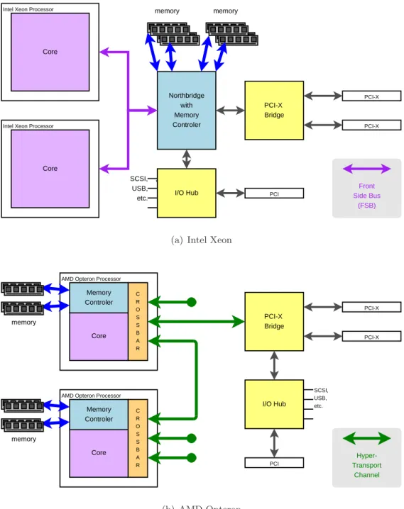
When comparing systems with Intel Xeon and AMD Opteron processors, one has to understand the differences in the architecture of the compared systems. Since this should only be a short introduction, this section concentrates on how the processors are connected with each other, with the memory of the system, and with the rest of the computer. For supplementary information on the AMD64 architecture please refer to [Vil02] and for a detailed comparison of the architectures with benchmarks refer to [Vil03]. Figure 2.5 illustrates the differences using [K¨oh05] as basis.

The main difference of the two designs is the way how the processors communicate with each other and the rest of the system. Where Intel uses an ordinary bus5_design,

AMD comes up with point-to-point links of which three are available per processor. For the Intel Xeon processor (Figure 2.5(a)), this means that every memory access (the memory is attached to the Northbridge) must share the bandwidth of the front side bus (FSB) with any inter-processor communication and the normal I/O of the

4

Fiber optic cables come in two different flavors: expensivemonomodefiber for long distances and

multimodefiber at lower price. The difference is that monomode fibers are that thin that the

signal propagates in a straight line, thus prohibiting the usage of multiple modes (see [Tan03, Section 2.2.4, pages 93 et. seqq.] for details).

5

A medium which is shared by all attached devices is called a bus. Therefore, it is necessary to separate the transfers from another. This design is fairly simple and well known.

(21)

2.4 Architecture Comparison: Intel Xeon vs. AMD Opteron 13/86

Intel Xeon Processor

Core

Intel Xeon Processor

Core Northbridge with Memory Controler PCI-X Bridge PCI-X PCI-X

I/O Hub PCI

SCSI, , USB, etc. memory memory Front Side Bus (FSB)

(a) Intel Xeon

Core Memory Controler C R O S S B A R PCI-X Bridge I/O Hub

AMD Opteron Processor

PCI-X PCI-X PCI SCSI, USB, etc. Core Memory Controler C R O S S B A R AMD Opteron Processor

memory memory Hyper-Transport Channel (b) AMD Opteron

Figure 2.5:Block diagrams of the designs of Intel Xeon 2.5(a) and AMD Opteron 2.5(b) for

comparison: Every Xeon processor is connected via the Front Side Bus with the Northbridge and with each other processor, whereas every Opteron processor has three independent HyperTransport Channels to communicate with other processors or system components. In the Opteron design, the memory is directly attached to the processors which is not the case for the Xeons having their memory attached to the Northbridge.

(22)

system. Elsewise AMD (Figure 2.5(b)), where every processor has its own memory. This grants fast access even if all three communication channels (called HyperTrans-port) are busy. To avoid interfering with the processor operation (core) for memory transfers, the memory can be accessed from any other processor via crossbars. The network interface cards used for our measurements are attached to the PCI-X bridge, because they need busses faster than standard PCI. Regarding packet cap-turing, both designs are equal in terms of copying hops from the network card to the main memory.

2.5 Network Traffic Characteristics

Since this thesis aims at a comparison of the performance of machines while packet capturing, it is necessary to provide traffic for that purpose. It is imprudent to use a random source for this objective because it has to match the characteristics of real network traffic. Therefore, it is inevitable to know these characteristics when searching for a suitable traffic source.

Research of local area networks (LANs) [LTWW93] as well as of wide area networks (WANs) [PF95] has shown that the traffic in common networks is best described as self-similar. This means that over a wide range of time-scales bursts can be identified. If, for example, the traffic is modelled as a Poisson arrival process, that would not be the case. Then the peaks would average out when looking at long enough time scales. This is not the case for real network traffic as [CB96, page 5, figure 2] and [WTSW97, page 24, figure 7] show. Network traffic is considered with fractal properties: Regardless of the scale similar structures can be observed. As reasons for this behavior [CB96] mentions file size distributions and superposition of many traffic sources. These sources depend on user bearing along which caching mechanisms. A more formal analysis of Internet traffic can be found in [CLS00, WTSW97].

The impact of these and other understandings in the field of network traffic charac-teristics is explained outstandingly in [FP01] in the context of simulating networks. When trying to simulate network traffic as demanded by the topic of this thesis, it is important to know about the above mentioned properties.

The subject of this thesis is to identify a way to capture all packets in transit from a link. When a system cannot keep up with bursts of the data rate, usually buffers are used to absorb peak rates. Thus, the system is for a while able to handle higher data rates than the average rate it can usually deal with. But keeping self-similarity in mind, for every imaginable buffer size there will be a long enough burst of the data rate to completely consume the available buffer space. So it is desirable to be able to permanently capture higher data rates than the average data rate of the traffic imposed on the systems. Thus, the intension is to find out how to capture packets at the highest possible data rate.

(23)

15/86

3 Methodology

Before performing any measurements, it is necessary to build up a testing environ-ment. Therefore, it is essential to define the requirements for this setup first. Then it has to be evaluated how the demands can be fulfilled.

3.1 Items in the Testing Environment

The influence of different factors on the capturing performance is to be evaluated. This thesis considers commodity systems only. But commodity hardware comes in different flavors with respect to processor architecture. There are IBM, Sun, Intel and AMD producing processors—just to mention the popular ones. Furthermore, there is the option to build multiprocessor systems or not, and a whole bunch of mainboards is available. The systems were chosen to represent the two most common dual processor architectures: AMD Opteron and Intel Xeon. This was done to be able to evaluate the benefit or penalty of multi-processor systems. To conduct a fair comparison, all systems have been purchased at the same time with comparable components and capacities. Using different architectures covers one major factor: the physical system throughput.

The other major factor can be covered by using different operating systems. Al-though there are many other operating system available like Windows, Solaris and MacOS X, this thesis concentrates on Linux and FreeBSD. There are two reasons for choosing the two: (i) these systems are the most popular ones in terms of packet capturing and (ii) they are Open Source and free of charge, thus everyone can use them. To be able to evaluate all operating system / architecture combinations, four systems are used in parallel for each measurement.

Besides of theseSystems under Test (SUTs) whose details are given in Section 2.3 and Figure 2.4, the following components are required for the intended measure-ments:

Workload Since packet capturing performance is to be tested, a source for the traffic which shall be captured is to be set up. This traffic has to be provided to all SUTs.

Transmission Media Because multiple systems have to be supplied with the same packets, it is necessary to find an appropriate connection of the source and the SUTs.

(24)

Capturing Application The traffic has to be captured. Therefore an application, which uses the same mechanisms as common network monitoring tools, has to be used. Furthermore, this can be used as a means of determining the performance.

Profiling The utilization ratio of the resources of the SUTs is helpful for an accurate evaluation. Therefore, an instrument for monitoring the CPU usage of the capturing machines is required.

3.2 Requirements

All of the above mentioned items have special requirements. Many of them have been identified during the project work described in [Sch04]. These will be discussed in the remainder of this section.

Systems under Test

The systems which were chosen for the measurement had to fulfill the following requirements.

• Different processor architectures are to be represented. In terms of architec-tures, AMD Opteron and Intel Xeon Systems are considered.

• Linux and FreeBSD, the two operating systems which are to be investigated, must run on these architectures.

• The network interface card used for capturing should be well supported by the considered operating systems. The Intel fiber Gigabit cards were chosen. Preliminary investigations have shown that this card is among the fastest well supported commodity cards.

• The PCI bus should be at least PCI-64bit aware for high throughput of the network cards. In fact, our systems can handle PCI-X as well but there are no commodity cards available for this bus.

Workload

Finding an appropriate traffic source for Gigabit Ethernet environments is a non-trivial task. The difficulty is to generate a reproducible sequence of packets at high speeds which is similar to real network traffic. In [Sch04] the Linux Kernel Packet Generator was utilized with different packet sizes ranging from 64 to 1500 bytes. But common network traffic usually consist of packets of the various sizes. So, the following three requirements have to be fulfilled:

(25)

3.2 Requirements 17/86

Speed The tool should be able to generate packets nearly at line speed (1 Gbit/s). If this requirement cannot be fulfilled, the load imposed on the capturing machines is not high enough to drop any packets. Therefore, a system bus faster than PCI is required. The throughput of standard PCI (32 bit, 33 Mhz) is at a theoretical maximum of 133 Mbytes/s which would just be enough for 1 Gbit/s. But taking into account that normally more than one device is attached to the PCI bus and that the capacity is shared by the devices, the effective throughput is reduced.

Realness The input for the SUT’s should be as similar as possible to real network traffic because, in general, it is necessary to capture genuine and not artificial traffic. The resemblance to real traffic should at least be satisfied with respect to the packet size distribution. This is important because different packet sizes produce distinct packet inter-arrival times, and different packet size distribu-tions generate varying packet rates (measured in packets per second—pps). This packet rate determines the interrupt rate which is directly influencing the capturing performance as described in Section 2.2. The type and content of the packets have no influence on the process of capturing. But since the sizes of the packets influence the required memory and the required costs for analysis, the packet size distribution should be as real as possible.

Reproducibility The sequence of packets should be identical across different mea-surements, especially with respect to the above mentioned requirements on realness. This is due to the fact that, otherwise, exceptional behavior or fail-ures are not reproducible and, therefore, cannot be examined in detail.

Transmission Media

Besides of actually transporting the generated traffic to the systems under test, it is necessary to supply the packets to all four capturing machines. Therefore, the traffic has to be duplicated several times. Based on our positive experience with passive optical splitters, they are used in this work.

In addition, an opportunity to monitor the traffic source in terms of number of generated packets is convenient to verify that all generated packets are indeed sent over the fiber.

Capturing Application

The capturing application has to be highly configurable to allow a wide range of possible settings. For example, it should be possible to apply filter expressions and configure additional load to simulate traffic analysis tools. In any case, it has to produce statistics on the number of packets received. To ensure compatibility and portability as well as relevance for real monitoring tools, the application needs to be build on top of libpcap.

(26)

Profiling

Regarding profiling, only two requirements have to be met. It has to be easy to use, and its impact on the system load should be small.

3.3 Test Setup

Considering these requirements a commodity system for workload generation, a switch, an optical splitter, the systems under test and a lot of wires were put together and form the test setup. Workload generation (Chapter 4) and profiling (Chapter 5) as well as the capturing application (Section A.1) are discussed separately.

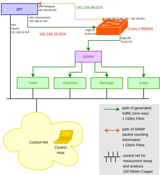
The test setup shown in Figure 3.1 is derived from the existing infrastructure (Fig-ure 2.3). All dispensable links were removed leaving the shown devices. The moni-toring link of the original setup described in Section 2.3 was replaced by a workload generator. The requirement of counting the number of generated packets is fulfilled by using a Gigabit (fiber) Ethernet Switch (Cisco C3500XL). The optical splitter is now attached to a port of the switch configured to monitor the input from the workload source.

The workload generator, called gen is a double processor AMD Athlon MP 2000 with a PCI-64bit bus (with 133 Mhz frequency) and a Syskonnect SK-98xx Gigabit (fiber) Ethernet controller. It is used to generate packets which can be captured simultaneously by all four sniffers to see which one loses how many packets. The second network card ingenis used to perform SNMP1 _{requests for the packet}

coun-ters of the switch. To avoid seeing these SNMP packets at the sniffers, a VLAN2 was configured for the two data ports (input fromgenand output to the splitter).

3.4 Measurement Cycle

To perform the measurements, it is necessary to synchronize the sender with the receivers. For this task a host within the control net (Figure 3.1) was chosen. This host performs the following steps as shown in Figure 3.2:

1. Login to the four sniffers to start the capturing and profiling applications. Save the process ID’s of these applications to designated files. Wait for all sniffers to become ready.

2. Login to gento read the SNMP packet counters of the switch. 1

SNMPis the simple network management protocol, which standardizes the communication be-tween different network devices.

2

A VLAN (Virtual LAN) separates different ports of a switch into different network segments. Usually there is no guaranty that packets arriving at a certain switch port are not sent out on another port. See [Tan03, Section 4.7.6, pages 328 et seqq.] for details on VLANs.

(27)

3.4 Measurement Cycle 19/86

gen

Cisco C3500XL

Splitter

swan moorhen flamingo snipe

Control Net 192.168.99.0/24 path of generated traffic (one-way) 1 Gbit/s Fibre path of SNMP packet counting information 1 Gbit/s Fibre

control net for measument setup and analysis 100 Mbit/s Copper GigE 0/6 VLAN 100 - 192.168.99.1 GigE 0/7 VLAN 101 GigE 0/8 VLAN 101 192.168.10.0/24 eth0 (Netgear) 192.168.99.100 eth1 (Sysconnect) 192.168.10.100 eth2 (3com) 131.159.15.200 Control Host

Figure 3.1: Network diagram of the setup of the capturing machines for measurements:

Instead of feeding the splitter with real network traffic as shown in Figure 2.3 another

computer (gen) is used to generate the packets which are to be sniffed.

3. Login to gen to start the packet generation. Proceed if the generation is finished and the statistics are saved.

4. Login togen to read the SNMP packet counters of the switch.

5. Login to the four sniffers to stop the applications using the saved process ID’s. Again, when all sniffers are done we can start a new measurement. To avoid strange behavior, this procedure is repeated several times.

(28)

gen

sniffer (all four at the same time)

control host super.sh start.sh capturing application profiling application snmp Couter Reading packet generation stop.sh forall data rates:

repeat measurement n times: data data data data data data data <<call start.sh>> <<start capturing>> <<start profiling>> <<call get-snmp.sh>> <<call get-snmp.sh>> <<call stop.sh>> <<start generator>> <<kill>> <<kill>> done done counter values counter values done

Figure 3.2: Sequence diagram of the measurement cycle: For each measured data rate, this

measurement cycle is repeated seven times to avoid outliers or unwanted influences. The action happens at three places: The host to control the measurement, the sniffers, and the generator. The red lines represent the generated packets.

(29)

21/86

4 Workload generation

The task of finding a proper tool for workload generation appears to be easy at first glance. But when exploring the range of available tools for packet generation, none of them matches the requirements from Section 3.2. A solution to this problem is presented in this chapter.

4.1 Existing Tools for Packet Generation

The following sections outline the advantages and disadvantages of existing free tools for generating packets.

4.1.1 TCPivo/NetVCR and tcpreplay

With reference to realness and reproducibility the best choice would be a program which replays a previously captured trace1 _{from a real network. Such tools include}

TCPivo/NetVCR2 _[FGB+_{03] and tcpreplay [Tur04].}

Replaying a trace of real network data meets the requirements of realness and repro-ducibility easily. The problem with these tools is the low maximum data rate they can produce. As Sebastian Lange showed in [Lan04, page 15 et seqq., figure 7 and table 2] the maximum transfer rate achievable with these tools is about 480 Mbit/s. Admittedly, the computer he used for generation had only a standard PCI bus. Yet, a test measurement usinggenreproduced his results (∼476 Mbit/s). This shows that such tools are to slow to generate traffic at line speed at the moment. In addition, the mentioned data generation rate is only possible with maximum sized packets.

4.1.2 “Monkey See, Monkey Do” and Harpoon

Monkey See, Monkey Do—described in [CHC+04]—is a tool for replaying live and online captured traffic from real networks into a test network for evaluating new network components or applications under real conditions. Since the output is the same as the input, another traffic source is needed. Furthermore, it does not focus

1

A collection of packets sniffed from a link is called atrace. Generally the packets of such traces are in order as captured from the link and provided with a timestamp.

2

The original name was NetVCR, but it was renamed to TCPivo due to name registration prob-lems.

(30)

on speed as it only replays what it captures. Therefore, it is no option for this work. The same holds for Harpoon [SB04] which does nearly the same, except that the output is generate based on statistics gathered from real networks.

4.1.3 Linux Kernel Packet Generator

The Linux Kernel Packet Generator (pktgen) [Ols02] is a Linux kernel module which can be used to generate UDP packets for network testing. It can be controlled via the/proc filesystem. Generated packets are sent as fast as the kernel is able. In contrast to the previously mentioned tools, the main advantage of the Linux Kernel Packet Generator is the speed with which it is generating packets. Data rates of up to about 938 Mbit/s on Gigabit Ethernet, which is nearly line speed considering Ethernet preamble, checksum, and inter-packet gaps, are achievable with a Syskonnect network card using 1 500 bytes sized packets. It is worth noting that the same measurement using a Netgear card results in 930 MBit/s or 890 Mbit/s using an Intel network card.

As mentioned in Section 3.2, the main disadvantage is its unhandiness since only one packet size can be configured. Mixing different instances of these kernel modules to produce different packet sizes is not possible without risking non reproducible data streams.

Besides these shortcomings, there are other interesting features. It is possible to configure an artificial inter-packet gap, setting the source and destination IP’s and MAC addresses, as well as cycling through such addresses.

4.1.4 Live Data

Our research group has the possibility to capture packets crossing the uplink of “a powerful communications infrastructure called the Munich Scientific Network (M¨unchner Wissenschaftsnetz, MWN)” (from [LRZ]) operated by the Leibniz Com-puting Center, a “joint comCom-puting center for research and education for all Munich universities” (from [LRZ]). This uplink connects the MWN with the G-WiN, “Ger-many‘s National Research and Education Network. It provides a high-performance infrastructure for the German Research and Education Community. [. . . ] Being con-nected to the European Backbone G´eant, G-WiN is an integral part of the worldwide community of research and education networks.” (from [DFN]).

The utilization of this Gigabit link ranges from about 220 Mbit/s (90 Mbit/s down-stream and 130 Mbit/s updown-stream) to about 1200 Mbit/s (400 Mbit/s downdown-stream; 800 Mbit/s upstream) at peak times. Data rates greater than 1024 Mbit/s are possible because this link is bi-directional, thus allowing 1024 Mbit/s inbound and 1024 Mbit/s outbound at the same time. This traffic is produced by 50 000 hosts.

(31)

4.2 Identification of Packet Size Distributions 23/86

The average rate (about 400 Mbit/s) is not high enough for the requirements of this thesis. But the systems must be able to capture and process the load of the link in production use. Among the applications running on the sniffers are Bro [LBN, Pax99], a free intrusion detection system for scientific research and fur-ther development, and a “time machine”3 [KPD+05, Kor05] for efficient recording and retrieval of high-volume network traffic.

But the biggest problem with this workload “source” is its non-deterministic output with respect to data and packet rate. This makes it really difficult to conduct com-parable measurements, not to mention reproducible measurements. Recapitulating, this source is totally inappropriate for performance measurements.

4.1.5 Summary

None of the available tools or sources is able to satisfy all of the requirements. Therefore, an existing tool has to be extended. The Linux Kernel Packet Generator is chosen as basis. The ability to generate packets of different sizes as well as a mechanism to feed a distribution of packet sizes to the generator has to be added.

4.2 Identification of Packet Size Distributions

Since the Linux Kernel Packet Generator has to be enhanced to generate packets of different sizes, the goal of this section is to examine the nature of real packet size distributions. First the characteristics of these distributions have to be identified before a representation model can be developed.

4.2.1 Analysis of Existent Traces

The first step is to identify the characteristics of packet size distributions of real network traffic. A short existing trace is analyzed with ipsumdump [Koh] to extract the packet sizes which are grouped by packet size and counted with an awk script. Comparing these results with [CMT98, page 8, figure 3(a)] shows that in our en-vironment the jumbo-frames4 _{of Gigabit Ethernet do not exist at all (compared to}

some few in [CMT98]). The distribution of packet sizes between 0 and 1500 Bytes is similar to [CMT98].

For larger trace files this proceeding proved to be very slow. Therefore, a small application in C was written to speed up the reading of trace files (see Section A.1

3

The idea behind thistime machine is to supply a mechanism for intrusion detection systems, to access interesting packets when they already have been transfered. If such a mechanism can be utilized, the intrusion detection system can apply a much stricter filter which reduces its load.

4

Ethernet frames are limited in size. The maximum size is 1500 Bytes. With the new Gigabit Ethernet specification so calledjumbo-frameswere created to raise this limit.

(32)

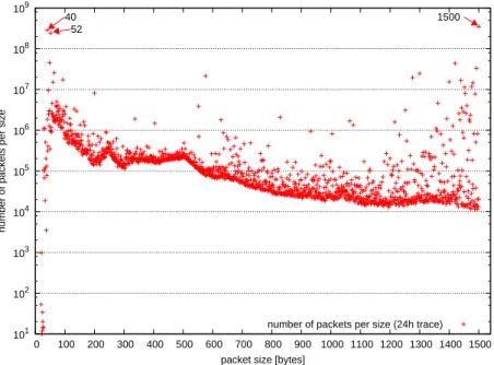
for details on this program). With the help of the new tool a twenty-four hour trace obtained at the uplink of the scientific network in Munich is examined to enlarge the data basis for the following calculations. The results are similar to those of the above mentioned trace. But at a different scale. The results are depicted in Figure 4.1 and it shows the usual peaks at 40–64, 552, 576 and 1420–1500 bytes.

4.2.2 Representing Packet Size Distributions

Because of the high packet rates that are to be generated, the representation of these kinds of distributions needs to be efficient but accurate. Using hash tables5 is too expensive because the size for each packet has to be looked up.

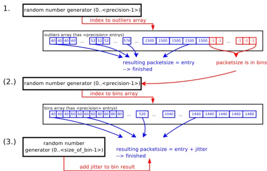
The goal is to match the sizes appearing often in the distribution with high accuracy. Unfrequent sizes do not need to be as accurate because more than three-quarter of the packets appear in the twenty most common packet sizes, see Figure 4.2. Using this insight, a two-stage system for representing such a packet size distribution is used. The desired procedure to achieve the packet size for the next packet is shown in Figure 4.3.

Needing a fast access method during the generation, the usage of simple arrays was chosen. Their content will be the packet size for the packets to generate. The variability comes in with the index to the entries of these arrays. The plan is to calculate a random number as index to the array entries and return the packet size of the indexed position.

The first stage uses the exact packet sizes with the probabilities of the heavy hitters (outliers). In our example, the heavy hitters are the twenty most often counted packet sizes of Figure 4.2. The second stage uses bins of configurable size in which multiple packet sizes are combined. These bins receive the sum of all included packet size probabilities as their own probability. This averages the diversity of the probabilities of the included packet sizes out, thus leading to a somewhat inaccurate output distribution. But it reduces the amount of memory needed and the time required to find the next packet size to a feasible extend. To allow the representation to be flexible, the following customizable parameters are used:

precision (ρ) This value can be used to change the size of the arrays. Smaller (larger) arrays lead to lower (higher) precision of the represented distribution. The default value is 1000.

5

A hash or hash table is a data structure which allows to save items with a large key space to

a memory as large as needed to contain the items. In general a hashing function is used to calculate an index from the key of the item. This index is shorter than the original key in terms of binary digits. See [CLRS03, chapter 11, pages 221 et seqq.] for details.

(33)

4.2 Identification of Packet Size Distributions 25/86 101 102 103 104 105 106 107 108 109 0 100 200 300 400 500 600 700 800 900 1000 1100 1200 1300 1400 1500

number of packets per size

packet size [bytes] 40

52

1500

number of packets per size (24h trace)

Figure 4.1: Scatterplot of an example distribution of packet sizes (y-axis in logscale): The

most frequent sizes can be identified at 40, 52 and 1500 bytes.

0 5 10 15 20 25 30 35 40 45 50 55 60 65 70 75 80 85 90 95 100 rest 1460 1470 1454 57 1452 44 1480 1440 1400 60 64 576 1300 1492 48 552 1420 52 40 1500 frequency/cumulated frequency [%]

packets of size (sorted by percentage descending) [bytes] cumulated relative frequency function

relative frequency of packets per size

Figure 4.2: Histogram plot of the percentages for the example distribution: Each packet

size from Figure 4.1 is shown with its fraction (green) of all packets. This plot also shows the cumulative sum (red) of the decreasingly sorted percentages from left to right. The three most frequently appearing packet sizes represent more than 55 % of all packets, and the top 20 packet sizes account for over 75 % of all packets.

(34)

Figure 4.3: Flow diagram: This figure shows how a new packet size is selected using the arrays. First an entry is chosen randomly from the outliers array. If the acquired packet size

(the value of the indexed position of the outliers array) is equal to −1 the searched packet

size was not yet found. Therefore, an entry from the bins array has to be selected randomly

and a jitter (with a randomly chosen amount between 0 andσbin−1) is added to the result

to obtain the packet size.

maximum packet size (Nps) The biggest packet size which will be considered by the distribution can be configured with this parameter. Its value defaults to 1500.

outliers boundary (p_Ωbound) This specifies how many packets relative to the total number of considered packets must be of same size, so that this packet size is associated with the first stage array. If this lower bound (default: 2h_{) is} exceeded, this packet size is called an outlier. Taking the topnmost frequently used packet sizes would also be possible but requires maintaining a list. binsize (σbin) This value specifies how many sequential packet sizes are merged into

one bin of the second stage array. Default: 20.

(number of bins) (nbin) nbin depends onσbin and Nps: nbin=

Nps

σbin

(35)

4.2 Identification of Packet Size Distributions 27/86

4.2.3 Calculation of the Resulting Distribution

This section explains the exact manner in which the arrays described in Section 4.2.2 are computed. The numbersciof packets of all sizes, where 0< i < Npsis the packet size, are assumed to be known as initial values. These values are obtained from a trace or a live capture. Furthermore, the number of all packets c_all can either be calculated or given as well. The following steps are performed:

1. The fractionspi are calculated from the number of packets per sizeci and the total number of packets call:

∀i: pi =

ci

c_all (4.1)

2. The set Ω of packet sizes which are outliers (first stage items) is identified, along with the number nΩ of outliers:

Ω ={i|p_i ≥p_Ωbound} n_Ω=|Ω| (4.2)

3. The bins—indexed byj—are generated (second stage items):

∀j∈ {1, . . . , nbin}: Ωj ={i|j·σbin≤i <(j+ 1)·σbin∧i∈Ω} (4.3)

nΩj =|Ωj| (4.4)

bj =

X

j·σbin≤i<(j+1)·σbin

i /∈Ω ci (4.5) avg_j = bj σ_bin−n_Ω_j (4.6) ∀i∈Ωj : ci=ci−avgj (4.7) bj =bj+avgj (4.8)

Before calculating the probabilities of any bin, the set Ωj of outliers for each bin have to be identified (4.3) and the number n_Ω_j of outliers in this set is counted (4.4). Within each of the bins the numbers ci of packets of size i are summed up in bj if the recent packet size is no outlier (4.5). Afterwards, the average frequency avg_j of the bin is calculated (4.6) and subtracted from the frequency of all corresponding outliers (4.7). Likewise, it has to be added to the frequency of the bin as many times as outliers have been found in the bin (4.8).

4. Now the probability of all outliers and bins can be calculated:

∀i∈Ω : poutl_i = ci

c_all ∀j∈ {1, . . . , n_bin}: pbin_j = bj

call

(36)

Because it is not possible to work with floating point numbers within the kernel, the Linux Kernel Packet Generator cannot be “fed” with floats. Therefore, this is done in user space while the following step transforms the floats into integers. This will produce arrays with packet sizes for randomized access:

5. The arrays described in Section 4.2.2 are generated with the number of cells

f_indextype which have to be filled with the same packet size:

∀i∈Ω : f_ioutl=ρ·poutl_i

∀j∈ {1, . . . , n_bin}: f_jbin=ρ·pbin_j (4.10)

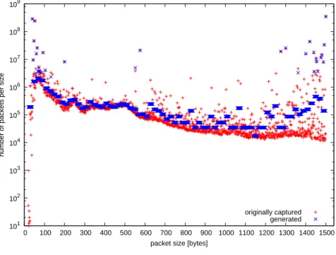
As shown in Figure 4.4 the distribution of the generated packet sizes is not perfect but matches the heavy hitters well. This can be easily recognized in the magnifica-tions of Figure 4.4(b), where the heavy hitters are located on the left. Figure 4.4(a) shows clearly the bins of the generation process. But it is close to the original distri-bution. For reasons of simplicity, the random numbers generated to index the arrays and to produce the jitter are equally distributed. This leads to similar frequencies for packet sizes in the same bin.

4.3 Enhancement of the Linux Kernel Packet Generator

The computation of the input—the arrays from the last section—for the enhanced packet generator is done by the same application (createDist, Section A.1) that is used for counting the different packet sizes.

To use these packet size distributions, it is necessary to change the source code of the Linux Kernel Packet Generator module [Ols02]. For a detailed list of changes as well as information on using, compiling, and obtaining this changes please refer to Section A.2.

4.3.1 Results

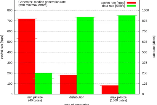
With a sample distribution similar to the one shown in Figure 4.1 packet rates of about 180.000 pps and data rates of about 915 Mbit/s (as shown in Figure 4.5) can be achieved. This corresponds to a nearly fully utilized Gigabit Ethernet link. The drop in the generated bandwidth—when compared to maximum sized packets—is negligible when considering the benefit of having a “real” packet size distribution. Another pleasing side effect in this comparison is the doubled packet rate. Since higher packet rates require faster interrupt processing and higher data rates require higher system throughput, both rates should be high to impose a remarkable load on the systems under test.

(37)

4.3 Enhancement of the Linux Kernel Packet Generator 29/86 101 102 103 104 105 106 107 108 109 0 100 200 300 400 500 600 700 800 900 1000 1100 1200 1300 1400 1500

number of packets per size

packet size [bytes]

originally captured generated

(a) Scatterplot (y-axis in logscale): packet size against frequency

101 102 103 104 105 106 107 108 109 number of packets

packets classified by size (sorted descending by quantity of packets) originally captured

generated

107 107

(b) Frequency plot (y-axis in logscale): All packets of the same size are joined in a class. These classes were sorted descending by the quantity of packets belonging to it. The discrepancy comes from averaging the frequency in bins.

Figure 4.4: These plots show the original (captured) distribution of packet sizes and the

(38)

This new method of generating packets meets all goals mentioned in Section 3.2. So the demands of this part are fulfilled. But the results also show that when high packet rates are needed it is better to use equally and minimum sized packets.

packet rate [kpps] date rate [Mbit/s]

type of generation

packet rate [kpps] data rate [Mbit/s]

0 100 200 300 400 500 600 700 800 max pktsize (1500 bytes) distribution min pktsize (40 bytes) 0 125 250 375 500 625 750 875 1000 Generator: median generation rate

(with min/max errors)

Figure 4.5: Histogram the packet and data rates generated by the Linux Kernel Packet

Generator: This figure shows how the generator performs with minimum and maximum sized packets in comparison to the new packet size distribution mechanism.

(39)

31/86

5 Profiling

One of the performance bottlenecks is the processing power of the machines perform-ing the packet capturperform-ing. On that account, it is interestperform-ing to know the utilization ratio of the processors during packet capture. Therefore, some sort of profiling is needed. At least the overall CPU usage should be recorded to be able to tell if the system was fully loaded or not. In this chapter the tool used for this task is presented.

5.1 cpusage

In order to be able to monitor the CPU load while capturing packets, a small appli-cation has been written in C, calledcpusage(Section A.3). It reads out the systems CPU accounting information. These are counters of how many tics the CPU spends in one of the following modes:

• user applications,

• niced (low priority) applications,

• system/kernel,

• idle,

• (Linux only:) input or output,

• interrupts,

• (Linux only:) soft-interrupts.

The total number of tics spend can be computed as the sum of all this counters. The modes marked as “Linux only” are counted as system/kernel or interrupts under FreeBSD.

The problem is that these counters are started at boot time and cannot be reset. Hence, the percentages cannot be calculated from a single readout. Instead, the counters have to be read twice. Then the differences between corresponding counter values yield the result. The percentages are acquired by dividing the differences by the sum of all differences.

Finally, the percentages for each mode are available. This is the same way how

(40)

.. .

user: 35.2%, nice: 0.0%, system: 3.1%, idle: 38.3%, interrupt: 23.4%, user: 32.8%, nice: 0.0%, system: 1.6%, idle: 35.9%, interrupt: 29.7%, user: 32.3%, nice: 0.0%, system: 1.5%, idle: 41.5%, interrupt: 24.6%, user: 10.9%, nice: 0.0%, system: 1.6%, idle: 68.0%, interrupt: 19.5%, user: 32.0%, nice: 0.0%, system: 3.1%, idle: 32.0%, interrupt: 32.8%, user: 33.9%, nice: 0.0%, system: 0.0%, idle: 39.5%, interrupt: 26.6%,

---Summary----Min: user: 10.9%, nice: 0.0%, system: 0.0%, idle: 32.0%, interrupt: 19.5%, Max: user: 35.2%, nice: 0.0%, system: 3.1%, idle: 68.0%, interrupt: 32.8%, Avg: user: 28.4%, nice: 0.0%, system: 1.6%, idle: 43.4%, interrupt: 26.6%,

Figure 5.1: Sample output of thecpusageapplication.

counters data is accessed. (Under FreeBSDsysctl1has to be used instead of a read to /proc/stat1 under Linux.)

cpusagereads the counters twice a second keeping the last readout at any one time for calculation and writes the calculated percentages to a file. This is like using

top, with the improvement of being able to go back in time. Another advantage compared withtopis a built-in minimum, maximum, and average percentage calcu-lation during the measurement. The periods of measurement or, in other words, the periods when packets are captured, are correlated with periods of heavy load. Thus,

cpusage assumes packet capturing if the load exceeds a configurable threshold. When trying to find out the average CPU usage for the time when the machine is capturing packets, the start and end times are difficult to define. According to the measurement procedure explained in Section 3.4 the profiling application is started far before the the packets are generated. Thus, the average accounting is started when the idle percentage drops below a user defined limit, and stopped when the same limit is penetrated again. A sample output is shown in Figure 5.1.

5.2 Postprocessing of the cpusage Results

In some measurements the calculated average values seem to be incorrect, because the value is too low to fit with the other comparative values. This happens, because

cpusage reacts the first time the idle value falls below the user defined threshold. If this is not caused by the capturing, the period determined for the average usage during the capturing is incorrect.

1

A sysctl under FreeBSD as well as the/proc filesystem under Linux are used to get and set kernel parameters.

(41)

5.2 Postprocessing of the cpusage Results 33/86

To solve this problem, a small awk script trimusage.awk (see Section A.4) was written which reads the unaggregated data (the lines before---Summary--- from Figure 5.1) and calculates the correct average values. To acquire the wanted result, the script reads all input lines and builds periods of times when the idle value is under-usage. When all lines have been read, the longest period is chosen as the one caused by the capturing. Then the average value is calculated from this block of lines.

For the plots in the following chapter these values are used, but the original is kept as well for supervision.

(42)