Computer Physics Communications

Contents lists available atScienceDirect

Computer Physics Communications

www.elsevier.com/locate/cpc

Linear-scaling density-functional theory with tens of thousands of atoms:

Expanding the scope and scale of calculations with ONETEP

N.D.M. Hine

a

,

∗

, P.D. Haynes

a

, A.A. Mostofi

a

, C.-K. Skylaris

b

, M.C. Payne

c

a_{Department of Physics and Department of Materials, Imperial College London, Exhibition Road, London SW7 2AZ, United Kingdom} b_{School of Chemistry, University of Southampton, Highfield, Southampton SO17 1BJ, UK}

c_{Theory of Condensed Matter group, Cavendish Laboratory, J J Thomson Avenue, Cambridge CB3 0HE, UK}

a r t i c l e i n f o a b s t r a c t

Article history:

Received 3 December 2008 Accepted 17 December 2008 Available online 24 December 2008 PACS:

31.15.es 71.15.-m Keywords:

Applications of density-functional theory Methods of electronic structure calculations

ONETEP is anab initioelectronic structure package for total energy calculations within density-functional theory. It combines ‘linear scaling’, in that the total computational effort scales only linearly with system size, with ‘plane-wave’ accuracy, in that the convergence of the total energy is systematically improvable in the manner typical of conventional plane-wave pseudopotential methods. We present recent progress on improving the performance, and thus in effect the feasible scope and scale, of calculations with ONETEP on parallel computers comprising large clusters of commodity servers. Our recent improvements make calculations of tens of thousands of atoms feasible, even on fewer than 100 cores. Efficient scaling with number of atoms and number of cores is demonstrated up to 32,768 atoms on 64 cores.

©2008 Elsevier B.V. All rights reserved.

1. Introduction

Density-functional theory (DFT) is well-recognized as a versa-tile and powerful tool for studying condensed matter systems[1]. While it is now widely used for predicting static and dynamic properties of molecules and solids, it is similarly widely recog-nized that conventional DFT methods become severely inefficient at large system sizes. In the conventional Kohn–Sham approach, the computational effort involved in a total energy calculation scales asymptotically as the cube of the system size, restricting the approach to the study of no more than a few hundred atoms. However, for almost as long as this limitation has been known, a parallel methodological track has been developing: that of linear scalingDFT[2].

A number of codes now exist which implement variations on this linear scaling approach, using a number of different choices of basis set and approaches taken to the optimization of the energy or diagonalization of the Hamiltonian[3–8]. The code addressed in this paper, ONETEP, combines the benefits of linear scaling with a level of accuracy and variational bounds comparable to that of tra-ditional cubic-scaling plane-wave approaches, often argued to be the most unbiased and controllably accurate method of perform-ing a DFT calculation.

The formalism of linear scaling [9]is general for all systems with an energy gap, as this guarantees the exponential

localiza-*

Corresponding author.

E-mail address:[email protected](N.D.M. Hine).

tion of the Wannier functions[10]. However, the demands of linear scaling vary considerably in different types of system, depending on the details of the periodicity, packing and electronic structure of the atoms involved. Most demonstrations of linear scaling DFT to date have focused on localized, finite systems or systems elongated in one or two dimensions, such as nanotubes, nanorods and slabs. Linear-scaling calculations in fully 3-dimensional-periodic systems, while possible within the framework, have remained challenging and time-consuming for reasons we will discuss. One useful mea-sure of the value of a linear-scaling approach is known as the ‘crossover point’, and is defined as the number of atoms in the system at which the computational time for a total energy calcu-lation becomes lower with a linear-scaling approach than with a traditional cubic-scaling approach of comparable accuracy. While it can be very low for isolated structures, this figure has remained high for fully-periodic solids treated with ONETEP, of the order of 300–500 atoms in favorable systems such as semiconductors, and up to 1000–1500 atoms in unfavorable systems such as metal ox-ides. To bring down this crossover, one must decrease the prefactor of the linear scaling by increasing the efficiency of the algorithms used.

ONETEP was developed from the beginning as a parallel code [11]. In this paper we will describe a number of improve-ments to the parallel algorithms of the ONETEP code, which have resulted in considerable speed-ups of almost all aspects of the package. Combined, these have enabled us to bring down the pref-actor of linear scaling considerably for all systems. For solids, in particular, calculations which would have been unfeasibly slow can 0010-4655/$ – see front matter ©2008 Elsevier B.V. All rights reserved.

now be regarded as routine, and the true linear-scaling regime is fully accessible even to inexpensive clusters of commodity servers. In Section 2 we will briefly outline the formalism used by ONETEP to achieve linear-scaling computational effort. We will then address some of the main challenges of practical implemen-tation of this formalism and recent improvements in their scaling with system size and their efficiency on parallel computers, in Sec-tions3, 4 and 5. Section3deals with the implementation of sparse matrix algebra and its varying performance in systems with dif-ferent sparsity characteristics. Section4 addresses the ‘row-sums’ operation common to many parts of the program, and Section 5 addresses successes in reducing and optimizing the use of Fourier transforms, which are in many cases the limiting factor on perfor-mance. Finally in Section 6we present benchmarks and demon-strations of linear scaling in various systems, over a wide range of sizes.

2. Theoretical background

Kohn–Sham DFT relies on the substitution of the real ing system by a fictitious system of independent particles interact-ing with a mean-field potential V

[

n

]

(

r

)

, which is a functional of the densityn

(

r

)

. The system is then described by the Hamiltonian

ˆ

H

ψ

n

(

r

)

=

− ¯

h 2m

∇

2

₊

_V

_[

_n

_]

₍

_r

₎

ψ

i

(

r

)

=

i

ψ

i

(

r

),

which must be solved self-consistently for the orthogonal single-particle states

{

ψ

i

(

r

)

}

with eigenvalues

{

i

}

. In a periodic system the orbitals are often labeled with a band indexiand a k-pointk, and known as Bloch orbitals. This system of noninteracting par-ticles thus described can equivalently be fully described by the single-particle density matrix

ρ

(

r

,

r

)

, which in terms of the Bloch states can be written as

ρ

(

r

,

r

)

=

i Vcell

(

2

π

)

3

BZ fik

ψ

ik

(

r

)ψ

i∗k

(

r

)

d3k

.

The integral is over the 1st Brillouin Zone (BZ), and occupation numbers fik of 0 or 1 correspond to empty or filled states

re-spectively. The charge densityn

(

r

)

is simply the diagonal part of the density matrix,

ρ

(

r

,

r

)

, multiplied by two if required to ac-count for spin-degeneracy. Any approach which involves calculat-ing and manipulatcalculat-ing these Bloch functions directly will inevitably scale as O

(

N3

)

: there must be at least O

(

N

)

orbitals to describe the O

(

N

)

electrons occupying them; each orbital extends over the whole system and thus any manipulation of it requires effort of O

(

N

)

; finally, the constraint of mutual orthogonality between these orbitals means that minimization of the energy can only be achieved with an extra O

(

N

)

computational effort.

The steps that enable linear scaling are, firstly, to realize that the total energy can be calculated and minimized without ever ex-plicitly calculating the energy eigenstates, and secondly that the density matrix is, in an insulator at least, ‘nearsighted’. The den-sity matrix can always be represented in terms of a set of localized nonorthogonal functions

{

φ

αR

}

, as

ρ

(

r

,

r

)

=

αβ

R

φ

αR

(

r

)

Kαβ

φβ

R

(

r

),

(1)

where we have also introduced thedensity kernel Kαβ _[12], repre-senting a generalization of occupation numbers to a nonorthogonal basis. The functions

{

φ

αR

}

are referred to as NGWFs

(Nonorthogo-nal Generalized Wannier Functions)[13], and can be thought of as a combination of a subspace rotationM

(

k

)

of the Bloch orbitals at

eachkand a unitary transformation ink-space, localizing them to a supercell at positionR:

φ

αR

(

r

)

=

V

(

2

π

)

3

BZ e−ik.R

i

ψ

ik

(

r

)

Miα

(

k

)

dk

.

Within ONETEP, these functions are expressed in terms of a ba-sis of periodic bandwidth-limited delta functions, or psinc func-tions [13,14], and are strictly localized to a spherical region of radius Rφα. These psinc functions, with coefficientsCi,α, are cen-tered on the grid points ri of a regular grid, the spacing of which is determined by a plane-wave cutoff energy Ecut with a similar meaning to that in a plane-wave code.

Given a set of NGWFs

{

φ

α

}

in the home simulation cell (such that R

=

0) and a density kernel

{

Kαβ

_}

_{, one can calculate the} Kohn–Sham total energy, expressed as

E

{

Kαβ

_}

_,

_{

_φ

α

}

=

KαβHβα

+

EDC

[

n

]

,

(2) where the first term is the bandstructure energy and EDC com-pensates for the double-counting of density interactions present in the first term. A summation is implied over repeated Greek in-dices throughout. The matrix elements of the Hamiltonian are con-structed for each pair of overlapping NGWFs by techniques which achieve linear scaling with system size by means of the so-called ‘FFT box’ technique described previously [15]. In this approach, the psinc functions are projected into a box of fixed size, gener-ally smaller than the simulation cell, which is then used for all Fourier transforms required to calculate the parts of the Hamilto-nian which are more easily treated in reciprocal space.

To find the ground state energy of a given system, one must minimize Eq.(2)simultaneously with respect to the density kernel elements Kαβ and the coefficients describing the NGWFs them-selves. ONETEP achieves this optimization by means of two nested loops: the outer loop optimizes the basis set by minimizing the in-teracting energy with respect to the NGWF coefficients, while the inner loop optimizes the density kernel by minimizing the energy for a given set of NGWFs with respect to the density kernel ele-ments. We express the outer loop as

Emin

=

min

{Ci,α}

L

{

Ci,α

}

,

(3)

where the coefficients Ci,α are nonzero only for psinc functionsi at points ri within the localization radius of

φ

α. The inner loop, performed at fixedCi,α, minimizes the energy with respect to the kernel elements Kαβ L

{

Ci,α

}

=

min {Kαβ_}E

{

Kαβ

_{}; {}

_C i,α

}

.

(4)

This minimization ensures that in Eq.(3), L is a function only of the coefficientsCi,α.

The technical details of the implementation of this scheme have been described in some detail elsewhere [8,11,13–18]. In this ar-ticle, we will discuss only the aspects of the scheme underlying the time-limiting steps of this calculation. By maximizing the ef-ficiency of these steps through consideration of the properties of typical physical systems, it is possible to extend the scope and scale of linear-scaling plane-wave DFT calculations to unprece-dented heights.

3. Sparse matrix algebra

Achieving true linear scaling of computational effort relies on the fact that the density kernel, expressed as a matrix in terms of the NGWFs in Eq. (1), is ‘nearsighted’. This means that the scale of matrix elements between distant NGWFs decays exponentially with the separation of the centers of these NGWFs: Kαβ _{can then}

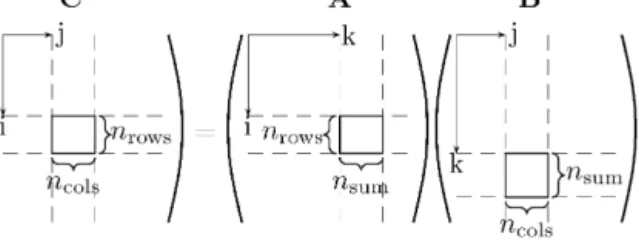
Fig. 1.Schematic representation of the multiplication of one pair of blocks during a sparse matrix multiplication in ONETEP. On the left is matrixC, the block shown of which contains a contribution from the blocks ofA and B, on the right. The dimensions of the blocks guarantee compatibility of the matrix sizes. Efficiency of these small block matrix-multiplication operations is crucial to the overall speed of the matrix algebra.

be truncated for NGWF centers separated by more than some cut-off length, when

|

Rα

−

Rβ

|

>

RK. This ensuresKhas a high degree

of sparsity in the limit of large systems, as each NGWF

φ

α has nonzero density kernel elements Kαβ _{only with a} system-size-independent number of other nearby NGWFs

φβ

. For a suitably chosen ordering of the atoms (achieved in ONETEP by means of a Peano space-filling curve [19]), the nonzero elements ofK are clustered near the diagonal of the matrix. For a set of strictly lo-calized functions

φ

α of rangeRφ the overlapSand HamiltonianH will also be short-ranged and thus sparse. Algebraic manipulation of these sparse matrices can therefore in principle be achieved inO

(

N

)

time given sufficient sparsity.

It is therefore crucial to the implementation of linear-scaling methods to have a sparse matrix algebra methodology capable of dealing efficiently with the multiplication of matrices whose spar-sity pattern corresponds to that of typical real systems of atoms. Previous descriptions of the parallel algorithms of ONETEP have fo-cused on the efficient parallel evaluation of operator integrals, and the sparse algebra routines have not previously been described: here we will briefly introduce the parallel sparse matrix algebra routines, and focus on how they have been optimized for efficient scaling.

All the matrices considered here are of sizeN

×

N where N is the number of NGWFs required to represent the occupied orbitals of the atoms present. This can exceed 105 in the largest calcu-lations presented in this work. The elements of the matrix must therefore be distributed over the parallel nodes of the computer running the simulation. The atoms are distributed over the nodes, and the data corresponding to columns of the sparse matrix are stored only on the node to which the atom of each column be-longs. The sparse indexing is dealt with by ‘atom-blocking’, where a block corresponding to the atom in column i and row j is of sizemi

×

mj, wheremi is the number of NGWFs on atomi. This means that rather than recording the NGWF rows for which each column is nonzero, we can record the atom block-rows for which each atom block-column is nonzero. This works because all the NGWFs for a species of atom have the same radius, so if any NGWF on a particular atom overlaps with one on another atom, they all do. Within the block, the data for each NGWF column is stored sequentially, and the computational overhead of indexing and cache-latency of sparse algebra is thus greatly reduced.

However, despite this efficient design, the performance of the sparse algebra routines has, in previous implementations of the method, been one of the main limiting factors on the speed of calculations, preventing efficient operation beyond a few thousand atoms. A first, relatively trivial step to improving this performance was to optimize the innermost loop of the sparse product by con-sidering the physical systems to which it will most often be ap-plied. Consider the operationCα_β

=

AαγBγβ, whereA,BandCare sparse matrices which may have different sparsity patterns.Fig. 1 shows this multiplication schematically. To perform the product,

three nested loops are required: first, over the block-columns j of B and C, parallelized over the nodes over which the atoms are distributed; second over all the nonzero block-rows k of B; and finally, for each block found, over the block-rowsi which are nonzero in bothAandC. If the data for the required block-column ofAis not local to the node on which the contribution from a par-ticular column ofBis being evaluated, it must be communicated to this node. There is therefore an outermost loop over the other nodes and, for each step, the nodes receive data from a different other node. Since each individual NGWF sphere only overlaps a system-size-independent number of its neighbors, there are only O

(

1

)

nonzero row elements in each column. This means that in principle the operation can be completed inO

(

N

)

operations over-all.

For one node–node pair, the pairs of blocks of A and Bthus identified as contributing toC are matrix-multiplied together and added to those of C. The fact that each matrix obeys the same blocking scheme means that the number of rowsnrowsin the block ofCis the same as inA, the number of columnsncolsin the block of C is the same as in B, and the number of columns nsum in the block of A is the same as the number of rows in the block of B. We therefore have three numbers nrows, ncols andnsum de-scribing the block-multiply. In principle, these can have any value, but some physical insight into the systems being simulated allows considerable speedup. Because the NGWFs in a particular atom-block represent anin situoptimized basis for that atom, one need only ever put enough NGWFs on each atom to represent the oc-cupied pseudo-atomic orbitals, taking into account the symmetry properties required due to their being centered on the atoms. For example, if only the uppermost s- and p-bands are occupied, 4 NGWFs are sufficient (1 to represent thesorbital and 3 for the px, py andpz orbitals). The overwhelming majority of block sizes in a real calculation are therefore in the set

{

1

,

4

,

5

,

9

,

10

}

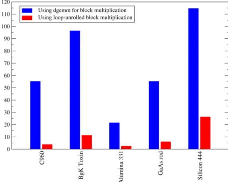
, depending on the species of atom and the nature of the bonding. By hard-coding the matrix multiplication for many of the combinations of these commonly occurring values, we avoid the overhead of library calls for these trivial matrix-multiplications.

The result, for simulations where the multiplication operations for the required block sizes are hard-coded, is a dramatic decrease in the total time taken for sparse algebra operations. A rough guide is a factor of 10 when executed on a single processor, though the specific value depends on the library call being compared against. However, this speedup in the time for the actual mathematical op-eration brings into clearer focus two further issues: firstly, that the communications patterns can be improved greatly by physical con-siderations of the optimal distribution of atoms over nodes for a realistic system, and secondly, that in many typical systems, the matrices being calculated are not, in comparatively small systems, of a great enough size that sparse algebra is actually worthwhile at the typical filling fractions that occur.Fig. 2 shows a compari-son of the time taken for 10 sparse matrix products when using generic matrix multiplication code, versus the time for the loop-unrolled version of the inner loop of the block multiplication. The range of systems tested is meant as a cross section of typical uses of the code demonstrating different challenges in different parts of the code, and is explained inTable 1.

Building on this success, we can obtain further system-de-pendent speedup by analyzing the properties of the dominant sparse algebra on which the main optimization cycle of the code relies, so as to alleviate the limiting factors on performance. ONETEP uses two approaches to the optimization of the density kernel: the penalty functional approach of Haynes and Payne[18] and our own modification of the Li, Nunes, Vanderbilt [20–22] variational approach. The latter is in use during the main loop of

Fig. 2.(Color online) Total time for 10 sparse matrix product operations on 4 cores of a dual-socket, dual-core Intel Woodcrest node. We compare the operation using the LAPACK routine ‘dgemm’ to the same operation with all the block multiplication operations unrolled for efficient vector operation.Table 1shows a key to the abbreviations labelling the systems.

Table 1

Key to the abbreviations used for the 5 different systems used for performance testing.

Abbrev. System Ecut/eV RK/a0 Rφ/a0 Nat Nφ Niter

C960 (12,0)carbon nanotube 400 20 6.7 960 3840 4

BgK toxin Organic anemone toxin 500 22 6.0 581 1466 10

Alumina331 α-alumina 3×3×1 cell 1200 24 7.7 270 1080 1

GaAs rod Wurtzite GaAs nanorod 400 40 10.0 430 1222 4

Silicon444 Silicon 4×4×4 cell 600 20 7.2 512 2048 1

Systems were chosen to represent a cross-section of common uses of ONETEP (nanostructures, organic molecules, semiconductor and oxide solids, etc.) and different extremes of cutoff energyEcut and kernel and NGWF cutoffsRK andRφ. The number of atomsNat and NGWFsNφare also shown. The numbers of iterationsNiter were chosen so as to keep the total times for each system comparable.

the program. In this approach, one defines the following electronic Lagrangian:

L

(

K

)

=

E

(

K

˜

)

−

μ

2 Tr

[ ˜

KS

] −

Ne

,

whereK

˜

is the McWeeny purified density kernel[12],

˜

K

=

3KSK

−

2KSKSK

,

(5)

andE

(

K

˜

)

is the total energy functional of this purified kernel. In-spection of Eq.(5)shows that if there is to be no truncation during the intermediate steps of updating the kernel, one must deal with matrices whose degrees of sparsity are very much lower than that of the kernel itself. For example, the least sparse matrix one cal-culates before the result is truncated has the form

(

KSKS

)

αβ, and this can be nonzero for any

φ

α,

φβ

pair separated by a distance

|

Rα

−

Rβ

|

of up to 2RK

+

4Rφ. This very greatly reduces the spar-sity of the resulting matrix, compared to that of the kernel itself. Furthermore, it is often desirable to be able to carry out calcula-tions with no kernel truncation, and not just in metals where the kernel cannot be truncated for physical reasons. Even though lin-ear scaling will not be obtained in very large systems, below a threshold of a few thousand atoms the computational time taken performing matrix algebra is negligible compared to other parts of the calculation.

Sparse matrix multiplication is only a benefit compared to sim-ply padding a full-square matrix with zeros as long as the over-head of sparse indexing is lower than the time saved by avoiding the unnecessary multiplication of zero elements. In practice, this

means that sparse matrices are not worth using unless they are around 90% sparse or more. It is therefore often possible to obtain a time saving by neglecting the sparse matrix indexing and sim-ply using a fully dense form for small systems. We have therefore implemented an option within ONETEP to activate dense matrix algebra in place of the sparse matrices.

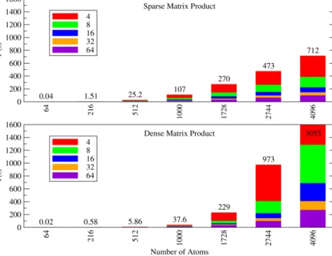
Comparisons of the performance of the two approaches can be seen in Figs. 3 and 4. Here we consider a typical sparse matrix product of a type which occurs many times per iteration. Denoting the sparsity pattern of the density kernel by K and the sparsity pattern of the overlap matrix by S, here we show an operation where the sparsity patterns of the matrices in the product are KS

×

K

→

KSK. For a typical solid, diamond-structure silicon, with Rφ

=

6

.

8a0 for the NGWFs and RK

=

24a0 for the density kernel, we consider supercells of Nat

=

8M3 atoms, resulting from repeating the 8-atom simple cubic unit cell M times in each direction. The degree of sparsity of these matrices as a function of the number of atoms in the supercell is shown in Table 2. Fig. 3 shows the timings for 10 repetitions of a matrix product between the two with both approaches. We vary both Nat and the number of CPU cores NP to show the scaling with the size the system and the number of cores used for the calculation.Fig. 4shows the timings for the matrix trace of a product of the same two matrices, which does not require evaluation of the full matrix product and thus scales differently withNat andNP.

The conclusion is as one would expect: dense matrix algebra is considerably faster at low filling fractions but scales as a much

Fig. 3.(Color online) Total time for 10 matrix product operations for matrices of typical sparsity levels for a solid, parallelized over varying numbers of cores. The overlayed colored bars represent different numbers of cores. The dimension of the matrix is 4Nat as there are 4 NGWFs per atom. Above: Block-indexed sparse matrices. Below: Fully dense matrices. Sparse algebra becomes linear-scaling withNat above a threshold of around 1000 atoms, whereas dense algebra remainsO(N3

). Sparse algebra therefore becomes faster somewhere around 2000 atoms. As the number of processors scales up, the total time scales down by nearly the same amount—the slight decrease from full 1/NP scaling of total time being due to the extra communication overhead at higherNP. AsNat increases, the maximum efficient value ofNPincreases with it.

Fig. 4.(Color online) Total time for 10 matrix trace operations for the product of two matrices of typical sparsity levels for a solid. Above: Block-indexed sparse matrices. Below: Fully dense matrices.

worse power of N: O

(

N3_at

)

for matrix multiplication, and O

(

N_at2

)

for the trace of a matrix product. With sparse algebra, the oper-ations respectively scale as O

(

N_at3

)

andO

(

N2_at

)

initially, while the filling fraction is still high, but both becomeO

(

Nat

)

above a certain system size, once the system already contains all the atoms within range of the various cutoffs. This occurs at aroundNat

=

1000 in the system shown here—beyond this point a graph ofT

(

Nat

)/

Nat would be seen to be flat as a function ofNat. Sparse algebra takes over as the faster method once we passNat

=

1728. At this point,

the kernel sparsity is 75% and the overlap sparsity is 95%, but the KS structure is still only 22% sparse and KSK is still at 0% spar-sity. As one would expect from the algorithm described above, it is clear that the sparsity of the multiplier and the multiplicand are more significant than that of the product in determining the time for the operation. These results appear to be typical for solids, though of course the rate at which the filling fraction changes with Nat depends on the values chosen for RK and Rφ and the crystal structure of the solid. The choices of localization radii used

Table 2

Filling fractions of matrices of different sparsity patterns for cubic supercells of fcc silicon. Nat S K KS KSK 64 93.75% 100.00% 100.00% 100.00% 216 40.28% 100.00% 100.00% 100.00% 512 16.99% 78.52% 100.00% 100.00% 1000 8.70% 44.10% 98.10% 100.00% 1728 5.03% 25.52% 77.78% 100.00% 2744 3.17% 16.07% 54.34% 100.00% 4096 1.73% 10.77% 35.23% 98.19% 8000 0.89% 5.51% 18.04% 73.15%

K is the sparsity pattern of the density kernel, which is cutoff atRK=24a0, and S

is the sparsity pattern of the overlap matrix, which is generated from the overlap of NGWFs of radiusRφ=6.7a0. KS is the sparsity patterns of a matrix product of

the kernel and overlap matrix, and KSK is the sparsity pattern of the product of this matrix with the kernel again.

Fig. 5.Sparsity pattern of the overlap matrix of a 512-atom block of solid silicon (M=4). Blocks shown in black represent atoms whose radius 6.7a0spheres

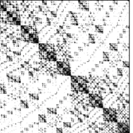
over-lap. The atoms have been ordered according to a Peano space-filling curve, which has the effect of grouping together nearby atoms, such that the nonzero elements cluster on the diagonal.

here correspond to a simulation able to match with a high degree of accuracy the results of a plane wave calculation of equivalent cutoff energy[23].

It is crucial that a linear-scaling DFT code scales efficiently to very large numbers of processors, as it is only in large systems that the benefits of the formalism will be obtained. Concurrent with the aforementioned improvements to the algorithms for the ma-trix algebra, and advantageous to its performance in both sparse and dense formats, we have implemented a new communications pattern for the sparse algebra routines. The importance of the com-munications pattern can be seen by considering the occupation of a typical matrix where the nonzero elements are determined by the overlaps of spheres centered on atoms ordered by a space-filling curve.Fig. 5shows a typical sparsity pattern for the overlap matrix in a block of the silicon system considered above. It can be seen that the space-filling curve is fairly successful in cluster-ing the nonzero elements of the matrix onto the diagonal even in a solid.

The consequence of this clustering is that the load balance must be carefully considered when performing matrix multiplica-tion. The atoms, and thus the matrix data, are distributed over the nodes of the parallel computer: All nodes must in general commu-nicate with all other nodes in order to perform a matrix multipli-cation, so the operation is divided into Np node-steps. However, there are multiple options for the ordering of the communica-tion and calculacommunica-tion. If the communicacommunica-tions pattern is such that at node-stepm all nodes work simultaneously on the portion of nodem’s data that overlaps their segment of the matrix, the load for that node-step will be very unevenly balanced, since clearly

node m will take very much longer on that node-step than any other node. We therefore order the communication so that each node first works on its own data, then steps off the diagonal by one to work on the next node’s data (modulo Np), then the next, and so forth. In this manner, each individual node-step is approxi-mately the same length on each processor.

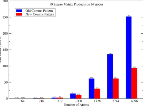
Fig. 6 compares the time taken for 10 sparse matrix multipli-cation operations with varying numbers of atoms on a 64 node cluster. With the old communications pattern, in which a ‘blocking’ communications operation (mpi_bcast) was used to communicate the data stored on each node to all other nodes at each step, sparse algebra performance was becoming severely limited by 64 nodes and large numbers of atoms. With the new system, the communi-cations algorithm improvements have resulted in more than a 50% speedup (over and above any speedup due to improved block mul-tiplication or dense matrix algebra).

As a result of considerable development work on the sparse algebra routines therefore, motivated by considerations of the physical system being studied, the sparse algebra performance of ONETEP has been sped up by a very considerable factor. On a small number of nodes this factor is around 10. However, the speedup scales with number of cores due to the removal of ‘blocking’ com-munications operations: on 64 cores, a factor of 20 or more can be obtained relative to the original implementation.

4. NGWF–NGWF pair operations

One of the main challenges of linear-scaling DFT is the evalu-ation of the entire Hamiltonian matrix with algorithms that scale as O

(

N

)

, in that each element of the Hamiltonian matrix is eval-uated with a computational effort that does not increase with the size of the system beyond a certain point. This is achieved in ONETEP by the use of the FFT box approach [15,16]. Several of the routines in ONETEP which employ the FFT box approach share many elements of their algorithmic structure, the common element of which we will describe as ‘row sums’. Considerable reduction in the prefactor of linear scaling can be obtained by ex-ploiting this similarity, which is the result of the common spatial localization of the NGWFs, to optimize the improve the perfor-mance of the algorithms used to evaluate various quantities.

The common structure of these routines can be seen by exam-ining the intermediates we must evaluate in order to calculate the following: (i) the kinetic energy Ekin via the kinetic matrix Tαβ, (ii) the local potential (sum of the Hartree and XC potentials and the local part of the pseudopotential) via the local potential ma-trix V_αloc_β, (iii) the densityn

(

r

)

, and (iv) a precursor to the NGWF gradient. Expressions for these are given below:

(i) Ekin

=

Kαβ

φ

α

| ˆ

T

|

φ

β

,

(ii) Eloc

=

Kαβ

φ

α

|

Vloc

|

φβ

,

(iii) n

(

r

)

=

Kαβ

_φ

α

(

r

)φβ(

r

),

(iv)

∂

E

/∂φ

α

(

r

)

=

Qαβ

φβ(

r

)

+ · · ·

where Qαβ _{is a matrix with the sparsity pattern of K}αβ_{. In each} case, the kernel (or other matrix of the same sparsity) is mul-tiplying what is effectively a matrix of overlaps or products of functions, and the distribution of NGWFs over nodes means that each node only needs to calculate those elements of this ma-trix where

φ

α belongs to that node. For each

φ

α, therefore, there are some number of NGWFs

φβ

for which some operation must be performed: for the kinetic energy, this is the Laplacian fol-lowed by calculation of the overlap with

φ

α, for the density, it is Fourier interpolation with

φβ

and deposition to the accumulat-ing FFT box, and so on. A full description of this system can be

Fig. 6.(Color online) Comparison of old and new communications patterns. Left bars: Blocking communications routines. Right bars: Diagonal-patterned nonblocking, com-munications routines. The performance gain achieved by this physically-motivated reorganization increases with the number of nodesNP. Already at 64 nodes the new

approach is more than twice as fast as with the blocking routines.

Fig. 7.Schematic 2D slice of an FFT box cut out of a rhombohedral unit cell, cen-tered onφα. Parallelepiped domains (ppds) within the sphere ofφαorφβonly are shown in light gray, and ppds within the spheres of bothφαandφβin dark gray. Calculations such as overlaps need only consider the ppds common to both spheres. For matrix elements such asφβ|∇2|φα, calculation of∇2φα(r)via a Fourier trans-form delocalizes it over the whole FFT box. However, one can still save computation by extracting the result to the ppds ofφβ summing the overlap only over these points, as elsewhereφβis zero.

found in Figs. 2–5 of Ref.[11] and the accompanying text, so we only summarize it here.

The

φβ

functions that overlap with each

φ

α will not necessarily be local to the node of

φ

α, so some communication of NGWFs is required. These NGWFs are stored in a so-called ‘ppd representa-tion’ (see Ref.[11]), where their values are recorded on the points inside a number of parallelepipeds (ppds) which are regions of the full simulation cell determined by division of the full grid in to parallelepiped-shaped regions of fixed numbers of points along each axis.Fig. 7shows a schematic representation of the benefits of the ppd approach.

Communication of NGWF values between processors is per-formed by sending lists of the ppds within the NGWF sphere, and the psinc coefficients on the points in those ppds. For large ra-dius spheres, this communication can take of order hundreds of microseconds, and there may be many millions of NGWF pairs to calculate per node. Additionally, because it is often not feasible to store the FFT boxes of every NGWF on each node simultaneously, a batch system is implemented so as to work on a batch of columns

at a time. A loop runs over batches of as many NGWFs as fit in memory, and having received each

φβ

, it is applied to every

φ

α in the batch with which it overlaps. However, if an NGWF

φ

βoverlaps multiple

φ

α functions in different batches, it must be recommuni-cated several times. Furthermore, the time taken to perform the inner operation (overlap or product) on each NGWF is small but not negligible, and serves to exacerbate any inefficiencies in the communications caused by any degree of serialization. It is there-fore of great importance to optimize the pattern of communication within a batch so as to maximize performance.

The communication pattern implemented prior to the current version is described in detail in Ref. [8]. Briefly, this consisted of a double loop, first over node–node blocks of the matrix start-ing with the diagonal, then over NGWF pairs for that block, all in synchrony between nodes. To avoid otherwise catastrophic seri-alization where columns have overlaps that need calculating only on a small number of processors at a time, the outer loop was per-formed in two stages. First, the node–node blocks on or below the diagonal were processed, eliminating one node-column from the calculation after each off-diagonal row. Second, the blocks above the diagonal were dealt with, again eliminating one node-column each time but in the reverse order to during the first stage, giving 2NP

−

1 steps in total. This ensured that the communication over-lapped calculation efficiently in as much as the limiting case was the calculations being performed on the first node during the first stage, and the last node during the second stage. However, in both stages, all the nodes could often actually only be performing com-putation (rather than just waiting to send NGWFs) on average a little over half the time. Communications therefore accounted for upwards of 50% of the time during this stage of the calculation, and could be considerably worse in the case of densely overlap-ping solids, where the large number of NGWFs required by the first node from the last node tended to overflow available MPI buffers and cause considerable further slowdown.

For the new approach, we note that it is a relatively simple task to prepare a list of the row–column pairs that need calcu-lating on each node for a particular batch of columns using the sparse matrix index. By calculating this ‘plan’ and sharing it with all the nodes before calculating the overlaps or products, an

op-Fig. 8.(Color online) Comparison of ‘planned’ and ‘unplanned’ communications patterns during the calculation of the density, plus modifications to deposition of functions to FFT boxes. Calculations performed on 4 dual-socket, dual-core nodes (16 cores) of Imperial’s CX1 machine (Intel Woodcrest CPUs). Left bars: Old system. Right bars: New system. All the systems show considerable improvement, the more so the more their NGWFs overlap. Crystalline solids show a particularly large speed-up, since they necessarily have a large number of densely overlapping NGWFs.Table 1shows a key to the abbreviations labelling the systems.

timized communications pattern is automatically available to each node. The maximum number of overlaps or products on any node is the number of ‘plan steps’np. A loop over this number of plan steps occurs on each processor, and for each step the node first examines the plan of every other node to determine whether it is required to send a new NGWF to that node. It then examines its own plan to determine whether it is going to receive a new NGWF from any node. Having done so (or loaded the NGWF into a buffer in the case where the plan calls for a local NGWF on that step), it proceeds to calculate the overlap for that row–column pair (or add the row function to an accumulating FFT box for that column in the case of products). In practice, the sending of the NGWFs can pre-empt the corresponding receipt, simply by looking ahead in the plan by a set number of steps to determine what to send.

Further speedups can be obtained by cache-optimization of the operation itself. In the case of the routines involving the overlap of a function represented by the grid point values on the ppds of a sphere with the grid point values of a function in an FFT box, we have removed all instances where the ppd was deposited to full 3D boxes. Instead, given that the values of the first function is only nonzero on the ppd points, the values of the second function can be extracted to the ppds of the sphere of the first function. Then, by multiplying the ppd values together as a column vec-tor, the overlap is obtained with far fewer operations. This speeds up the calculation of the local potential and kinetic matrices con-siderably. A similar procedure works to speed up the density and NGWF gradient ‘row sums’

_β∩α

φβ(

r

)

. Because the multiplication of

φ

α

(

r

)

and

φβ(

r

)

must be performed on the fine grid to avoid er-rors due to aliasing, one must deposit the values of

φ

β

(

r

)

to an FFT box, in order to use Fourier interpolation. By streamlining this pro-cess into a straightforward ppd-by-ppd deposition of values rather than an extraction to a minimal box followed by a deposition of this box to the FFT box, the use of intermediate arrays has been removed. This results in a speedup of more than a factor of two in cases where this memory transfer was occurring outside of cache due to the size of the FFT box.

Figs. 8–10show the effect of these changes on the time taken to perform the parts of the calculation that can be limited by row

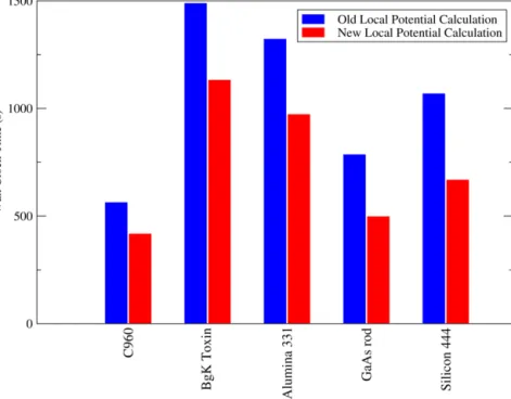
sums. Fig. 8 shows the time taken for a full calculation of the density across various systems, which are varyingly more or less dominated by the batch row sums part. Figs. 9 and 10 show the times for calculation of the local potential and kinetic matrices re-spectively. All of these show significant improvements, particularly the density evaluation.

5. Optimization of NGWF gradient and Fourier transforms

The outer loop of the calculation is the minimization of the to-tal energy with respect to the NGWF coefficients—effectively an optimization of the minimal basis set. To minimize the energy ac-curately with respect to these coefficients one must be able to calculate both the functional and the gradient of the functional with respect to the coefficients. The main computational effort of this optimization is divided into two parts: minimizing the elec-tronic Lagrangian using the LNV approach (the inner loop), and calculation of the energy gradient in the space of NGWF psinc function coefficients (the ‘NGWF gradient’). The full expression for the NGWF gradient varies according to the scheme being used, but for the psinc coefficient of a particular NGWF

φ

α corresponding to the point atri, it always takes the general form

δ

E

δ

Ci,α

=

β

[ ˆ

H

φβ

]

(

ri

)

Aβα

+

γ

φ

γ

(

ri

)

Bγα

,

for some choice of matrices Aβ

α and Bγα. In Section 4 we de-tailed improvements to the row sums, which is used for the latter expression, but this is often only a minor part of this calculation. Considerably more demanding, usually, is the calculation of the first part—the Hamiltonian acting on the NGWFs.

In the Hamiltonian, we can combine the Hartree VH

(

r

)

and exchange-correlation Vxc

(

r

)

terms (calculated directly from the density) with the local pseudopotential Vps,loc

(

r

)

to form a to-tal local potential Vloc

(

r

)

. We then need to consider only three separate terms: kinetic energy, local potential, and nonlocal pseu-dopotential. We are therefore calculating, on the grid points inside the localization radius of each

φ

α, the following expression

Fig. 9.(Color online) Comparison of ‘planned’ and ‘unplanned’ communications patterns during the calculation of the local potential matrix, combined with the effect of calculating of overlap integrals by extracting the functions from FFT boxes to ppds. Left bars: Old system. Right bars: New system.

Fig. 10.(Color online) Comparison of ‘planned’ and ‘unplanned’ communications patterns during the calculation of the kinetic matrix, combined with the effect of calculating of overlap integrals by extracting the functions from FFT boxes to ppds. Left bars: Old system. Right bars: New system. Those systems where the FFT time dominates over the communications and ‘row sums’ part have not improved significantly. However, those with densely overlapping long ranged NGWFs, particularly the crystalline solid systems still show an improvement.

β∩α

[ ˆ

H

φ

β

]

(

r

)

= −

1 2

∇

2

β∩α Kαβ

φ

β

(

r

)

+

Vloc

(

r

)

β∩α Kαβ

φ

β

(

r

)

+

β∩α

μ∩β Kαβ

_Pμ

_|

_φβ

Dμ Pμ

(

r

),

where Pμ are the nonlocal projectors and Dμ the corresponding Kleinman–Bylander denominators, labeled by an index

μ

which runs over the projectors for each angular momentum state on each atom with nonlocal channels in its pseudopotential.

A batch system has previously been partially implemented for this part of the calculation, but only for the local potential extrac-tion part. One batch of accumulating FFT boxes contains the ‘row sums’

_βKαβ

_φβ(

_r

₎

_{on the points in the FFT box centered on}

_φ

α, with the sum over

β

including all the NGWFs

φβ

overlapping

φ

α. The local potential Vloc

(

r

)

in the region for which

φ

α is nonzero must be extracted from the distributed, whole-cell array in which it is stored. One can therefore save on repeated extraction of the local potential if the FFT box containing

φ

α has not moved from

Fig. 11.(Color online) Comparison of old and new systems for the calculation of NGWF gradients. Improvements include the ‘planned sums’ system for calculating the accumulating FFT boxesβφβ(r), the saving of repeated calculations of identical projectors, and improvements in Fourier interpolation and Fourier filtering. Considerable speedup has been obtained across all systems—again, particularly those with densely overlapping NGWFs. Left bars: Old system. Right bars: New system.

one NGWF in the batch to the next (as will often occur since there are multiple NGWFs on each atom).

This batch system has now been extended to cover the nonlocal potential part of the calculation. Previously, for each

φ

α, there was a loop over the projectors overlapping all the

φβ

functions over-lapping

φ

α. If a projector contributed to the sum, it was generated from its reciprocal space radial representation once per NGWF

φ

α. However, since there are multiple NGWFs on each atom requiring the same projector at the same position in their FFT box, the batch system allows us to calculate these projectors only once per batch. This represents a very considerable saving on time spent Fourier transforming and shifting the projector functions.

To avoid errors due to aliasing, the calculation of local potential contribution is performed by multiplying the FFT box and the local potential together on the fine grid (which has twice the spacing of the standard grid). This routine has been improved considerably by improvements to the Fourier interpolation routines. By careful consideration of cache efficiency, and by avoiding unnecessary re-peated normalizations, the routines have been uniformly sped up by around 40%.

Fig. 11shows the combined effects of these improvements. The total time for calculation of the NGWF gradient is shown for the same set of different systems as the previous figures. In this case it is the GaAs nanorod, with its large radius NGWFs, and hence large FFT boxes, that takes longest—and also shows the greatest speedup as the overhead of recreating projectors is removed.

6. Results

In the preceding sections, we have detailed changes to the ONETEP code designed to improve the absolute speed of the code and its scaling with both system size and number of processors. We will now examine the overall effects of these changes. Most significant is the improvement in sparse algebra, which, in systems where this was the limiting factor (generally speaking, anything both well into the linear-scaling regime and larger than around 4000 atoms), has improved in performance by a factor of at least 5–10, and more on larger numbers of cores. Second, in solid sys-tems, where row sums performance was limiting on large numbers

of nodes, the optimization of these routines has resulted in a fac-tor of 5–10 (more system dependent) speedup in these areas of the code. Considerable work has also gone in to optimizing the initial-ization routines. Previously these contained many O

(

N2

)

steps that took negligible time and were thus judged not to matter as they were only performed once per calculation, such as initialization of the ppd lists describing each sphere. However, as the system size grows these inevitably grow to become comparable to the O

(

N

)

steps. However, most have now been replaced by alterna-tive algorithms which have onlyO

(

N

)

scaling, greatly reducing the initialization time. The only remaining algorithms scaling worse than O

(

N

)

are the Ewald sum (which is rarely a significant con-tribution to the total time) and the initialization of the whole-cell structure factor for each species, which is O

(

N2

₎

_{. There are} meth-ods available to improve the scaling of Ewald sums to O

(

N1.5

₎

_or better[24], and in even larger systems Fast Multipole Methods[25] may be the answer to calculating these long range electrostatic in-teractions in O

(

N

)

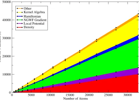
but at present the system sizes involved are not large enough to necessitate their use. Overall, for a full single-point energy calculation for a system size over a few thousand atoms and on a few tens of cores or more, the new code (version 2.2.12) is typically a factor of between 3 and 10 times faster than the pre-vious most recently-reported version (version 2.0.1).

Fig. 12 shows the total time for one full iteration of the code on cubic supercells of fcc silicon of increasing size. Full compari-son against previous versions of the code would be unfeasible for the systems shown here, due to the amount of wall clock time re-quired even for a single iteration of the old version at the larger system sizes. The results display near-perfect linear scaling of the total time per iteration at system sizes up to 32,768 atoms. The only limitation preventing larger systems from being tested on this hardware was the memory per core, which was nearly full by 32,768 atoms on 64 cores at this cutoff energy. Spreading the calculation over 256 cores or more would enable a 100,000 atom equivalent calculation. The number of NGWF iterations required for convergence remains roughly constant with system size, not ex-ceeding around 12–14, due to the efficient preconditioning of the gradient[14].

Fig. 12.(Color online) Timings for one iteration of ONETEP 2.2.12 on 64 cores (16 dual-socket, dual-core nodes) of Imperial’s CX1 cluster, calculating the total energy of a supercell of diamond structure silicon of increasing size. The total compute time is broken down by color into the various tasks performed each iteration. The dominant tasks are the calculation of the electron density (red), matrix algebra during kernel optimization (yellow), and calculation of the NGWF coefficient gradient (green). This calculation converges in around 12–15 iterations, independent of system size.

Fig. 13.(Color online). Total timings on 4 dual-socket, dual-core nodes (16 cores) for the most recent version of the code, 2.2.12, compared against those for version 2.0.1, which was current at the time of previous reports (e.g. Ref.[23]).Table 1shows a key to the abbreviations labelling the systems.

InFig. 13, we show the total times for the range of systems pre-sented above (note the varying number of iterations between dif-ferent systems, chosen to keep the total time approximately equal for easier comparison). Considerable improvements have been ob-tained across the range of systems, up to as much as an order of magnitude. Combined with the improved scaling with number of cores, this represents a very large increase in the feasible scale of problems that can be tackled with this approach. The sparse algebra improvements are at their most significant in systems pre-viously dominated by sparse algebra time, such as the 960-atom segment of carbon nanotube, so this shows the greatest improve-ment of all the systems. However, it is the speedup of the densely

overlapping systems such as the 3

×

3

×

1 Alumina supercell (120 atoms) which is most significant in terms of extending the range of applicability of ONETEP. Previously, it would not have been fea-sible on medium-sized clusters to access the linear scaling regime, the onset of which in a system with such large NGWFs is upwards of 1000 atoms since the number of points in an FFT box continues to grow as O

(

N3

)

up to this point. With the six- to ten-fold in-crease in performance of the row sums routines, such calculations are now routine on clusters of 16 or more cores.

The prevailing trend in high performance computing is towards ever larger clusters of high-performance, high-memory nodes

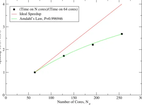
com-Fig. 14.(Color online) Parallel scaling for one iteration of the 27,000 atom silicon system fromFig. 12, on 64 to 256 cores of HECToR. The ‘speedup’ is normalized to be equal to 1 at 64 cores (the smallest number on which this calculation fits in memory). Also shown is the ideal speedup (NP/64) and a fit to Amdahl’s Law[26], which estimates

the parallel fractionP=0.9969.

posed of standard server CPUs connected with high-performance interconnects such as Infiniband. Consequently, it is important to know how a code scales to such large clusters. Previous results have demonstrated scaling of ONETEP from 1 to

∼

100 cores, and shown near-perfect parallelization, in that the wall clock time falls as nearly 1

/

NP with increasing number of cores. However, as one improves the serial performance of the code so that the paral-lel overheads become more significant, and as one goes to larger numbers of cores, it becomes harder to maintain this scaling. This is true of many applications: for example, a common way of us-ing traditional plane wave codes to simulate nonperiodic systems is to perform calculations on a large supercell at the Gamma-point only. One does not then benefit from the parallelization ofk-points over nodes, and while performance gains from parallelizing the code overG-vectors are rapid at small numbers of cores, commu-nications overheads come to dominate over around 100 cores and minimal further improvement is obtained.

In ONETEP, communications overheads are very much less, as they are only a serious issue within the sparse algebra routines. InFig. 14we present results obtained on a large cluster consisting of AMD Opteron dual-core nodes, the EPCC’s HECToR machine. We show the speedup relative to the time for the calculation on 64 nodes on 64, 128, 192 and 256 cores. There remains considerable improvement to be obtained even up to 256 cores, which is nearly a factor of 3 faster than with 64 cores, but clearly the improvement is beginning to saturate due to communications overheads. A fit to Amdahl’s law[26](which predicts the maximum speedup possible for an algorithm of which only a fractionP can be parallelized) fits the data well. At larger system sizes or with larger cutoffs this sat-uration point will come at a higher number of cores. Additionally, compared to a traditional plane-wave calculation at the gamma point (i.e. not benefiting fromk-point parallelization), Fig. 14 rep-resents very much more favorable improvement with system size. It is worth noting that, with the exception of the sparse algebra routines, all other parts of the calculation scale almost perfectly as 1

/

Np. Further work on the parallel scaling of the sparse algebra routines is expected to improve this performance.

7. Conclusion

We have presented a combination of improvements to the ONETEP code obtained by consideration of the factors limiting per-formance in typical systems. Sparse matrix algebra perper-formance has been sped up by the largest factor, but there are also very no-table improvements to the performance of many of the other tasks the code performs.

The scaling with the number of cores has been improved con-siderably. Previous results had shown this to be nearly linear in ideal systems such as nanotubes, but in solids performance be-came limited by communications inefficiencies at large system sizes. Now, with much more efficient parallel algorithms, use of the code in solids of thousands or tens of thousands of atoms has been demonstrated to be fast and efficient.

Acknowledgements

One the authors (N.D.M.H.) acknowledge the support of the En-gineering and Physical Sciences Research Council for postdoctoral funding (EPSRC Grant No. EP/F010974/1, part of the HPC Software Development program). P.D.H. and C.-K.S. acknowledge the support of University Research Fellowships from the Royal Society. A.A.M. acknowledges the support of the RCUK fellowship program.

Of great importance to this work was access to the comput-ing resources of Imperial College’s High Performance Computcomput-ing service (CX1), which has enabled most of the results presented here. Additionally, for the ability to perform larger calculations we acknowledge the computing resources provided by the EPSRC on the HECToR machine of the Edinburgh Parallel Computing Centre (EPCC).

References

[1] M.C. Payne, M.P. Teter, D.C. Allan, T.A. Arias, J.D. Joannopoulos, Rev. Mod. Phys. 64 (1992) 1045.

[2] S. Goedecker, Rev. Mod. Phys. 71 (1999) 1085.

[3] J.M. Soler, E. Artacho, J.D. Gale, A. García, J. Junquera, P. Ordejón, D. Sánchez-Portal, J. Phys.: Condens. Matter 14 (2002) 2745–2779.

[4] D.R. Bowler, R. Choudhury, M.J. Gillan, T. Miyazaki, Phys. Stat. Sol. B 243 (2006) 989.

[5] J. VandeVondele, M. Krack, F. Mohammed, M. Parrinello, T. Chassaing, J. Hutter, Comput. Phys. Comm. 167 (2005).

[6] J.-L. Fattebert, J. Bernholc, Phys. Rev. B 62 (2000) 1713; J.-L. Fattebert, F. Gygi, Phys. Rev. B 73 (2006) 115124. [7] M. Challacombe, J. Chem. Phys. 110 (1999) 2332.

[8] C.-K. Skylaris, P.D. Haynes, A.A. Mostofi, M.C. Payne, J. Chem. Phys. 122 (2005) 084119.

[9] G. Galli, M. Parrinello, Phys. Rev. Lett. 69 (1992) 3547.

[10] C. Brouder, G. Panati, M. Calandra, C. Mourougane, N. Marzari, Phys. Rev. Lett. 98 (2007) 046402.

[11] C.-K. Skylaris, P.D. Haynes, A.A. Mostofi, M.C. Payne, Phys. Stat. Sol. B 243 (2006) 973.

[12] R. McWeeny, Rev. Mod. Phys. 32 (1960) 335.

[13] C.-K. Skylaris, A.A. Mostofi, P.D. Haynes, O. Diéguez, M.C. Payne, Phys. Rev. B 66 (2002) 035119.

[14] A.A. Mostofi, P.D. Haynes, C.-K. Skylaris, M.C. Payne, J. Chem. Phys. 119 (2003) 8842.

[15] C.-K. Skylaris, A.A. Mostofi, P.D. Haynes, C.J. Pickard, M.C. Payne, Comput. Phys. Comm. 140 (2001) 315.

[16] A.A. Mostofi, C.-K. Skylaris, P.D. Haynes, M.C. Payne, Comput. Phys. Comm. 147 (2002) 788–802.

[17] C.-K. Skylaris, P.D. Haynes, A.A. Mostofi, M.C. Payne, J. Phys.: Condens. Matter 17 (2005) 5757.

[18] P.D. Haynes, M.C. Payne, Phys. Rev. B 59 (1999) 12173. [19] M. Challacombe, Comput. Phys. Comm. 128 (2000) 93. [20] X.-P. Li, R.W. Nunes, D. Vanderbilt, Phys. Rev. B 47 (1993) 10891. [21] M.S. Daw, Phys. Rev. B 47 (1993) 10898.

[22] P.D. Haynes, C.-K. Skylaris, A.A. Mostofi, M.C. Payne, J. Phys.: Condens. Mat-ter 20 (2008) 294207.

[23] C.-K. Skylaris, P.D. Haynes, J. Chem. Phys. 127 (2007) 164712. [24] J. Perram, H. Petersen, S. DeLeeuw, Mol. Phys. 65 (1988) 875. [25] L. Greengard, V. Rokhlin, J. Comput. Phys. 73 (1987) 325. [26] G. Amdahl, AFIPS Conf. Proc. 30 (1967) 483.