Virtual Scanning Algorithm for Road Network Surveillance

(1)

Virtual Scanning Algorithm for

Road Network Surveillance

Jaehoon Jeong,

Student Member, IEEE,

Yu Gu,

Student Member, IEEE,

Tian He,

Member, IEEE

,

and David H.C. Du,

Fellow, IEEE

✦

Abstract—This paper proposes aVIrtual Scanning Algorithm(VISA), tai-lored and optimized for road network surveillance. Our design uniquely leverages upon the facts that (i) the movement of targets (e.g., vehicles) is confined within roadways and (ii) the road network maps are normally known. We guarantee the detection of moving targets before they reach designated protection points (such as temporary base camps), while maximizing the lifetime of the sensor network. The main idea of this work isvirtual scan

– waves of sensing activities scheduled for road network protection. We provide design-space analysis on the performance of virtual scan in terms of lifetime and average detection delay. Importantly, to our knowledge, this is the first work to study how toguarantee target detection while sensor network deteriorates, using a novel hole handling technique. Through the-oretical analysis and extensive simulation, it is shown that a surveillance system, using our design, sustains orders-of-magnitude longer lifetime than full coverage algorithms, and as much as ten times longer than legacy duty cycling algorithms.

Index Terms—Sensor Network, Road Network, Virtual Scanning, Surveil-lance, Detection, Protection.

1 INTRODUCTION

Surveillance for critical infrastructure and areas is regarded as one of the most practical applications of wireless sensor networks (WSNs). So far, most of WSN surveillance systems have focused on surveillance for two-dimensional spaces, such as open battle-fields [1]–[4]. Research on road network surveillance, however, is very limited. In modern warfare, roadways (as fast maneuver paths) are vantage areas for military surveillance and operations. Clearly, surveillance in a road network is significantly different, because (i) the movement of targets (e.g., vehicles) is confined within road segments, and (ii) the road network maps are normally known (e.g., from Google Earth and Yahoo Maps). We argue that legacy solutions, which are not tailored for road networks, lead to suboptimal performance.

This paper proposes a novel sensing scheduling algorithm for target intrusion detection, utilizing the unique features of road networks. Specifically, we focus on supporting military operations with fast, infrastructure-free deployment. As shown in Figure 1(a), we guarantee the detection of targets, entering from entrance points, before they reach one of protection points; in modern

• Jaehoon Jeong, Yu Gu, Tian He, and David Du are with the Department of Computer Science and Engineering, University of Minnesota, Twin Cities, 200 Union Street SE, Minneapolis, MN 55455.

E-mail:{jjeong,yugu,tianhe,du}@cs.umn.edu.

Entrance Point Protection Point 4 2 1 2 3 1 2 3 4 4

(a) Protected Road Network

E E E E P P P P split merge Sensors wake up consecutively

Scan

Detect!

Road Intersection Sensing Scan 1 2 3 1 2 3 4 4

(b) Concept of Virtual Scanning Fig. 1. Road Network Surveillance

warfare, battlefield situational awareness requires both entrance points and protections points (e.g., temporary base camps) to be assigned and changed on demand for fast military maneuver within a road network. Therefore, we cannot place sensor gatesa priori before protection points for intrusion detection. Instead, a road-network-wide deployment is needed.

A straightforward solution for road network surveillance isduty cycling, in which nodes wake up simultaneously for w seconds (the minimum working time before reliable detection can be reported) and then the whole network remains silent forTseconds. The detection is guaranteed if it takes more thanT seconds for a target to travel along the shortest path between any pair of entrance points and protection points; this duty-cycling-based algorithm performs much better in terms of system lifetime than traditional full coverage algorithms [1]–[4] in road networks. This is because the duty cycling algorithm allows the whole network to be silent completely for T seconds everywseconds, but the full coverage algorithms (e.g., the one covers all intersections) require at least one subset of sensors to be active at any given point time, taking no advantage of the linear structure of road networks.

In this paper, we present a novel scan-based algorithm, which improves further energy efficiency of surveillance in road net-works. As shown in Figure 1(b), sensors wake up one by one for w seconds along road segments, creating waves of sensing activities, called virtual scanning. Waves propagate from one (or multiple) protection point P, split at the intersections, and merge along the route until they scan all of the road segments under surveillance. Our study reveals that this scan-based method can achieve significantly better performance (e.g., ten times system lifetime) than duty cycling algorithms. The concept of virtual scan-ning is simple, however, in-depth design is very challenging due to

(2)

a set of practical issues we consider in this paper. Particularly, we investigate (i) how to optimize the network-wide silent durationT

between scan waves, (ii) how to coordinate the working schedules of individual sensors during the scan, and (iii) how to deal with sensing holes due to unbalanced initial node deployment, node failure and the depletion of node energy over time. Specifically, the intellectual contributions in this paper are as follows:

• A new architecture for surveillance in road networks. VISA is the first work tailored for road networks, leading to orders-of-magnitude longer system life for target intrusion detection, using a novel scan-based algorithm.

• A sensing scheduling algorithm for an arbitrary road network. The working schedule of each sensor (i.e., when to wake up) is constructed in a decentralized way. The network-wide silent duration is computed byVISAscheduler and naturally disseminated along with sensing waves to the nodes in a network.

• An optimal sensing hole handling algorithm for uncovered road segments. The VISA scheduler deals with both the initial sensing holes at the deployment time as well as the sensing holes due to the heterogeneous energy budget among sensors by optimally labeling additionalpseudoprotection or entrance points.

• Considerations on two practical issues: (i) Detection failure probability and (ii) Time synchronization error. For each issue, we propose an optimal solution in terms of network lifetime.

The rest of this paper is organized as follows: Section 2 describes the problem formulation. Section 3 explains the VISA system design. Section 4 evaluates our algorithm through simula-tion. We summarize related work in Section 5 and then conclude this paper with future work in Section 6.

2 PROBLEM

FORMULATION

The goal in this paper is to choose each sensor’s sensing schedule in order to maximize the lifetime of a sensor network, while ensuring all intruding targets are detected before they reach protection points. For clarity, this section explains the basic idea of virtual scanning, using one road segment, and then we extend our design to arbitrary road networks in Section 3.

Dense area Sparse area Dense area Road Segment Length = l

E 1 2 3 n n-1 n-2 . . . . . . P . . .

Fig. 2. Randomized Linear Deployment

2.1 Virtual Scanning for Surveillance

We assumensensors are randomly placed on a road segment of lengthl. Each sensor has a conservative sensing circle of radius

r, which is long enough to cover the width of the road. This assumption holds true for most commercially available sensors (e.g., PIR sensors can detect moving car 60∼100 feet away). Therefore, we can represent sensing coverage using a linear sensor

network model as shown in Figure 2, wherensensors are linearly placed. At the moment, let the left end of the road segment be the entrance pointE of targets and the right end of the road segment be the protection pointP.

Letwbe the minimum working time needed by a sensor in order that the sensor can reliably detect a target over multiple samplings. Letvbe a maximum target speed. Suppose that targets enter only from the entrance point and move towards the protection point. In this scenario, we can use the traditional full coverage algorithms where sensors turn on all the time. We call this approach the

Always-Awake.

A better design can be built based on the observation that it takes at least l/v seconds for a target to pass a road segment of lengthl at a maximum speedv. Therefore, all sensors in the road segment can sleep togetherforl/v seconds, which is defined as silent time of the road network. After thissilent time, all nodes wake up simultaneously for detection. We call this approachDuty

Cycling.

n . . . . .

(b)

Sensor sensing sequence

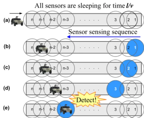
n-1 n-2 n-3 3 2 1 n . . . . . (c) n-1 n-2 n-3 3 2 n . . . . . (d) n-1 n-2 n-3 3 1 n . . . . . (e) n-1 n-3 3 2 1 n . . . . . (a)

All sensors are sleeping for timel/v

n-1 n-2 n-3 3 2 1

1

2

n-2

Detect!

Fig. 3. Sensor Sensing Sequence

Based on the fact that targets move only along the roadways, we propose a new design called Virtual Scanning. As shown in Figure 3, after all sensors sleep forl/vseconds, we turn on sensors one by one for working time w from the rightmost sensor s1 toward the leftmost onesn. Clearly, this wave of sensing activities guarantees the detection and allows additional sleeping time for individual sensors. Compared with Duty Cycling, this additional sleeping time is obtained by the fact thatall sensors but one can sleep during the scan. We note that the direction of a virtual scan shall be from the protection point to the entrance point. The virtual scan of the opposite direction (i.e., from the entrance point to the protection point) cannot guarantee target intrusion detection, if a very fast target enters right after the beginning of the network-wide silent time.

2.2 Analytical Network Lifetime Comparison

To understand key design parameters, this section compares an-alytically the network lifetime among the Always-Awake, Duty CyclingandVirtual Scanningmethods. For clarity, we summarize the notation in Table 1 and overall analytical results in Table 2.

Always-Awake & Duty Cycling: For the Always-Awake

ap-proach, the network lifetime Tnet is the same as Tlif e, because sensors work continuously without sleeping. For theDuty Cycling approach, the network lifetime Tnet is the number of periods

(3)

TABLE 2

Performance Analysis for Three Approaches

Approach Sleeping (Tsleep) Working (Twork) Network Lifetime (Tnet) Avg. Detection Time

Always-Awake 0 Tlif e Tlif e 0

Duty Cycling _vl w ⌊Tlif e

w ⌋(w+ l v) l2 2v(wv+l) Virtual Scanning (n−1)w+ l v w ⌊ T_{lif e} w ⌋(nw+ l v) l 2v TABLE 1

Notation of Parameters for Analysis

Parameter Definition

Tlif e Lifetime that a sensor can work continuously

corresponding to its energy budget.

Tnet Sensor network lifetime.

Twork Working time that a sensor needs to work for

reliable detection. NormallyTwork=w.

Tsleep Sleeping time of each sensor.

Tscan Scan time that a virtual scan wave moves along

the road segment.Tscan=nw.

Tsilent Silent time that the whole sensor network remains silent; that is, time that a target passes through the road segment of lengthl.Tsilent=l/v.

Tperiod Schedule period of the sensor network.

Tperiod=Tscan+Tsilent.

⌊Tlif e_w ⌋ multiplied by the length of the period Tperiod (i.e., the sum of the silent time _vl and the working timew):

Tnet =⌊Tlif e

w ⌋(

l

v +w) (1)

Virtual Scanning: In theVirtual Scanning, the network lifetime

Tnet is the number of periods ⌊Tlif e_w ⌋ multiplied by the period lengthTperiod.Tperiodis the sum of the scan time nwand silent time _vl as shown in Figure 4. Therefore, we have:

Tnet=⌊ Tlif e w ⌋(Tscan+Tsilent) =⌊ Tlif e w ⌋(nw+ l v) (2) 1 23 k n-1 n ... ... Time [sec] 0 P ow e r [m W ] w Twork= period T 1 23 k n-1 n ... ... nw Tscan= Tsilent=l/v

Scan Time Silent Time

Fig. 4. Scheduling Time Diagram for Nodek

Figure 5 shows the comparison of lifetime among these three approaches. For example, forw= 1sec,Virtual Scanninghas the lifetime of 30 hours, Duty Cycling3.2 hours, and Always-Awake 0.14 hour;Virtual Scanninghas 9.4 times lifetime ofDuty Cycling and 214 times lifetime of Always-Awake.

2.3 Analytical Detection Time Comparison

This section compares the average detection time after a target entering a road segment among the Always-Awake,Duty Cycling andVirtual Scanningmethods.

Always-Awake & Duty Cycling: For Always-Awake, since a

target is detected as soon as it enters the road segment, the average

0 1 2 3 4 5 0 5 10 15 20

Working Time w [sec]

Avg. Detection Time [sec]

Virtual Scan Duty Cycling Always−Awake 0 1 2 3 4 5 0 20 40 60

Working Time w [sec]

Network Lifetime [hr]

Virtual Scan Duty Cycling Always−Awake

Fig. 5. Performance Comparison according to Working Time

detection time is zero. For the Duty Cycling, if a target enters during the working period, detection time is zero. On the other hand, if a target enters during the silent time, average detection time is half of the silent time l/(2v). The percentage of silent time within a period isl/(wv+l), therefore, the overall average detection time of theDuty Cyclingapproach is l2_/₍₂_v₍_wv₊_l_)).

Virtual Scanning: We suppose thatnsensors are deployed on a

road segment, so each sensor covers the length ofl/nin average. Also, we suppose that target speed is v and a target can arrive at any time; that is, the arrival time is uniformly distributed. A target can arrive either duringscan timeorsilent time. We analyze separately the average detection time for each period and then combine them to obtain overall expected delay l/(2v). Please refer to Appendix A for detailed derivation; note that the average detection time for bounded variable target speed is also derived in Appendix B.

Figure 5 shows the comparison of average detection time among the three approaches. Virtual Scanning detects with a constant delay l/(2v) regardless of working time w. On the other hand, the average detection time of the Duty Cycling tends to de-crease slowly while working timewincreases. TheAlways-Awake method detects without any delay. For example, for working time

w = 0.1 sec, Virtual Scanning has similar performance with Duty Cycling, about 10.9 sec. For working time w = 5 sec, the Virtual Scanningdetects target within 10.9 sec in average and the Duty Cycling does within 8.87 sec; the average detection delay ratio between theVirtual Scanningand theDuty Cyclingis 1.23. However, the ratio of the Virtual Scanning’s network lifetime to the Duty Cycling’s network lifetime is 37, as shown in Figure 5. Thus, even though the average detection time increases slightly with Virtual Scanning, the benefit of network lifetime is quite remarkable.

2.4 Configuring VISA for Better Delay and Longer Life-time

As a reminder, when the network silent time Tsilent is equal to or smaller than l/v, target detection is guaranteed. Basic VISA design uses l/vas the network silent time Tsilent. However, if a smaller silent timeTsilentis used, it is possible to detect the target not only faster but also with less energy than theDuty Cycling algorithm.

(4)

0 10 20 30 0 5 10 15 20

Silent Time α [sec]

Virtual Scan Duty Cycling 0 10 20 30 0 20 40 60 80 100

Silent Time α [sec]

Network Lifetime [hr]

Virtual Scan Duty Cycling

α

min=2.5 sec αmax=21.6 sec

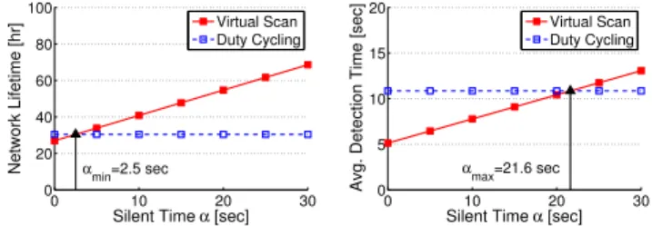
Fig. 6. Performance Comparison under DifferentαValues

LetTsilent =αforα∈ [0, l/v]. In order to outperformDuty

Cyclingin both network lifetime and average detection delay, we shall satisfy the following inequalities:

Virtual Scanning Duty Cycling

⌊Tlif e w ⌋(nw+α) ≥ ⌊ Tlif e w ⌋(w+ l v) l(nw+α) 2(nwv+l) ≤ l2 2v(wv+l) (3)

Solving the above inequalities, we have: max{l v−(n−1)w,0} ≤α≤min{ l(nwv+l) v(wv+l) −nw, l v}

When α falls into this range, Virtual Scanning has better performance thanDuty Cyclingin both the average detection time and network lifetime. For example, as shown in Figure 6, for

w= 0.1 sec, whenα is less than αmax = 21.6 sec, the average detection time of Virtual Scanning is shorter than that of Duty Cycling. Also, when α is greater than αmin = 2.5 sec, Virtual

Scanning’s lifetime is longer thanDuty Cycling’s. Thus, the range of α achieving better detection delay and lifetime is [2.5, 21.6] sec. We note the results here only illustrate the idea. Detailed study on the performance effect of αis presented in evaluation Section 4.3.

3 VIRTUAL

SCANNING

ALGORITHM

DESIGN

For the sake of clarity, the previous section presents the basic idea using one road segment. In the rest of the paper, we demonstrate how to apply the virtual scanning to road networks with arbitrary topology. This section is organized as follows: Section 3.1 lists definitions and assumptions used in VISA. Section 3.2 describes the scheduling algorithm, and Section 3.3 presents the hole handling algorithm.

3.1 Definitions and Assumptions

Definition 3.1 (Road Network Graph): Let Road Network Graph be G = (V, E), where V = {v1, v2, ..., vn} is a set of intersections, entrance points, and protection points in the road network under surveillance, and E = [eij] is a matrix of road segment lengtheij for verticesviandvj. Figure 7 shows a graph G corresponding to the road network in Figure 1. Note that the entrance point set and the protection point set are not static. These two sets can be changed either on demand for military maneuvers or to deal with sensing holes in Section 3.3.

Definition 3.2 (Network Lifetime): LetNetwork Lifetimebe the duration from the starting of a sensor network for surveillance until a target can possibly reach one of the protection points without detection. In other words, lifetime ends when there exists a possible breach path between an entrance point to a protection

1 9 2 10 3 11 14 15 12 13 5 6 7 18 8 16 17 4 200 80 200 150 140 130 70 100 250 110 170 100 140 180 160 150 140 110 140 270 150 250 140 80 E E E E P P P P

s

G

Fig. 7. Road Network GraphG

point. Note that for the target, we cannot differentiate between energy vehicles and our vehicles from detection since binary sensors are used.

Definition 3.3 (VISA Scheduler): LetVISA Schedulerbe a sink node that initiates the sensing scheduling algorithm.

The VISA design is based on the following assumptions: • Road map and locations of sensor nodes are known to

VISA Scheduler. The sensor location can be obtained through localization schemes [5].

• Sensors are roughly time-synchronized at tens of millisecond level. It can be easily achieved because existing solutions [6], [7] can achieve microsecond level accuracy.

• Sensors only have simple sensing devices for binary target detection, such as PIR sensors [8]. No sophisticated hardware is available.

• The circular sensing model is used in the conservative way using the minimum sensing range. For irregular sensing modeling, SAM [9] can be used to explore in-situ sensing irregularity.

• One of existing low-duty-cycle data forwarding schemes, such as DSF [10] and DESS [11] is used to deliver nodes’ locations and target detection results to the VISA scheduler. • Targets move only along predefined roads with the bounded

maximum speed.

3.2 VISA Scheduling on Road Network

This section presents the design of virtual scanning, including schedule establishment and dissemination.

3.2.1 Establishment of Working Schedule

For clarity in presentation, we use the subgraphGs of the graph G shown in Figure 7 where the edge weight means the physical distance of the road segment. First, we will consider a road network with one entrance and one protection point at first, and then will consider a road network with multiple entrances and multiple protection points. Also, for now, we assume that no sensing holes exist in the middle of roadways where targets cannot be detected due to the non-existence of sensors. The sensing hole handling will be discussed in Section 3.3.

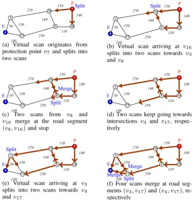
Figure 8 shows the snapshots of virtual scanning in the road networkGswith one entrancev4labeled asEand one protection point v7 labeled as P; note that one edge e3,4 of length 50 is added to Gs in order to explain the virtual scanning. The virtual scan’s propagation time on each road segment is the multiplication of the number of sensors and the individual working time w,

(5)

E P 3 8 16 17 4 Split 150 140 110 140 270 150 250 140 7 18 50

(a) Virtual scan originates from protection pointv7and splits into

two scans Split E P 3 8 16 17 4 150 140 110 140 270 150 250 140 7 18 50

(b) Virtual scan arriving at v16

splits into two scans towards v3

andv8 E P 3 8 16 17 4 150 140 110 140 270 150 250 140 7 18 50 Merge Split

(c) Two scans from v8 and v16 merge at the road segment

(v8, v16)and stop E P 3 8 16 17 4 150 140 110 140 270 150 250 140 7 18 50

(d) Two scans keep going towards intersections v3 andv17,

respec-tively E P 3 8 16 17 4 150 140 110 140 270 150 250 140 7 18 50 Split

(e) Virtual scan arriving at v3

splits into two scans towards v4

andv17 E P 3 8 16 17 4 150 140 110 140 270 150 250 140 7 18 50 Merge Split Merge

(f) Four scans merge at road seg-ments(v3, v17)and(v4, v17),

re-spectively

Fig. 8. Virtual Scanning on Road Network for Working

Schedule Establishment

instead of the physical distance of a road segment. As shown in Figure 8, by turning on sensors along roads consecutively, virtual scanning waves propagate along multiple routes simultaneously, split at intersections, and disappear when two waves encounter each other in a road segment. Note that once a virtual scanning wave arrives at entranceE, it keeps propagating to the rest of the road network. This scanning gurantees the detection of all of the mobile targets in the road network.

In the case of multiple entrance and protection points, scan operation is similar, except that multiple protection points initiate scanning at the same time. Because the waves merge in the middle of road segments during virtual scanning (as shown in Figure 8(c)), regardless the number of protection points and the locations of the sensors, each sensor only works forwseconds per scan, which is a nice feature for energy balance. Clearly, the scan wave arrival time for each sensor can be easily computed with All-Pairs Shortest Path algorithm, such as Floyd-Warshall algorithm[12]. We note the scan wave arrival time decides the working schedule of a sensor node. In other words, a sensor shall start to work for w

seconds after a virtual scanning wave arrives.

Road Network Virtual Scan 1 p 2 p n p . . . 1 e 2 e m e . . .

P

E

(a) Virtual Scanning on an Arbi-trary Road Network with Protec-tion Points and Entrance Points

1 p 2 p n p 1 e 2 e m e

P

E

. . . . . . . . . Scan Wave Propagation Path Vehicle Movement Path scan SP move SP

P

1 p 2 p n p

(b) Sleeping Time Computation considering the Shortest Scanning and Movement Paths

Fig. 9. Virtual Scanning on Road Networks

3.2.2 Establishment of Sleeping Schedule

The previous section discussed how to decide working sched-ule during the scan. This section explains how to compute the optimal sleeping length, i.e., the maximum duration sensors can sleep safely after working for w seconds while guaranteeing the detection.

Figure 9(a) shows the virtual scanning in an arbitrary road network. Let P = {p1, ..., pn} be the set of protection points.

Let E={e1, ..., em} be the set of entrance points. As discussed

before, a period Tperiod consists of (i) silent time Tsilent during which the whole network is turned off and (ii) scan time Tscan during which scan waves propagate across the network. Since a sensor only works for fixedTwork=wseconds everyTperiod, the longerTperiodis, the better energy efficiency we have. Therefore, we shall identify the maximum Tperiod value that can guarantee the detection. Before this optimization, we define two important concepts as below:

Definition 3.4 (The Shortest Scanning Path): The Shortest Scanning Path pscan(i, j) is the shortest-delay path for wave propagation from vi to vj on the graph G, where vi ∈ P and vj ∈E. Letlscan(i, j) be the number of sensors along the path pscan(i, j). Therefore, the Shortest Scanning Time Tscan(i, j) can be computed aslscan(i, j)∗w.

Definition 3.5 (The Shortest Movement Path): The Shortest Movement Path pmove(i, j)is the shortest-distance path between vertices vi and vj on the graph G where vi ∈ E and vj ∈ P. Let lmove(i, j)be the shortest distance ofpmove(i, j). Therefore, the Shortest Movement Time Tsilent(i, j) can be computed as lmove(i, j)/vmax, where vmax is maximum target speed. We note that all of the sensors along the path pmove(i, j) can sleep together for the silent time Tsilent(i, j).

These two shortest pathspscan(i, j)andpmove(i, j)for all pairs of vertices can be computed based onGby the All-Pairs Shortest Paths algorithm, such asFloyd-Warshall algorithm.

An important principle of computing the sleeping time is that all of vehicles entering during the sleeping time must be detected before their arrival to the protection points. Once a virtual scan wave originating from the protection points has swept an entrance point, the paths from this swept entrance point to the protection points are vulnerable to the target intrusion. This is because the swept paths are not swept again until the next scan period.

It is noted that we can guarantee detection by setting Tperiod as the sum of all-pair minimum scanning time and all-pair

minimum movement time. However, the resulting Tperiod is

shorter than the optimal value, (i) because an intruding target could have to travel a longer route from an entrance point with theearliestscan arriving time than the shortest route withall-pair

minimum movement time, or (ii) because it could have to wait

until a late scan arrives before it can travel along the shortest route with all-pair minimum movement time, especially when sensors are non-uniformly placed across a network.

We claim that a longer safe period Tperiod can be obtained as the minimum sum of the scanning time from vi to vj and

the vehicle movement time from vj to vk, for vi, vk ∈ P and

vj ∈ E than the sum of all-pair minimum scanning time and

(6)

a three-column graph is introduced as shown in Figure 9(b). The edges between the first and second columns denote the time for wave propagation and the edges between the second and third columns denote the time for target movement. To compute a safe period Tperiod, we need to identify the shortest path from any vertex in the first column to any vertex in the third column. Without loss of generality, supposep1⇒e1⇒p2is the shortest path where p1 ⇒ e1 is the shortest scanning path from p1 to e1, e1 ⇒ p2 is the shortest movement path from e1 to p2, and the sum of the scanning time and the movement time for these two paths is the minimum among all of the possible ones. Once the virtual scan arrives at the entrance pointe1 with a delay of Tscan(p1, e1), the path from the entrance pointe1to the protection point p2 becomes vulnerable, if the network remains silent for more thanTsilent(e1, p2). Thus, to prevent a target from reaching the protection pointp2without detection, another scan wave must be generated from the protection point p2 after Tsilent(e1, p2). Thus, the safe period isTperiod=Tscan(p1, e1) +Tsilent(e1, p2). Note that p1 ⇒ e1 and e1 ⇒ p2 are not necessarily all-pair minimum scanning path and all-pair minimum movement path simultaneously. Therefore, our claim is proved. Consequently, the sleeping time is Tsleep = Tperiod−Twork, because each sensor must work for its duty cycleTwork=wseconds per period.

Now, we can formally define the optimization problem of the sleeping time. Suppose that sensors are randomly deployed into the target road network with a uniform sensor density; note that since the number of sensors is proportional to the road segment length, the shortest scanning path is the same as the reverse of the shortest movement path. Let Tsleep(i, j, k) = Tscan(i, j) + Tsilent(j, k)−Tworkforvi, vk ∈Pandvj ∈EwhereTwork=w. The optimal sleeping time is chosen as follows:

Tsleep← min

vi,vk∈P, vj∈E

Tsleep(i, j, k).

(4) Obviously, the searching for an optimal sleeping time is done in polynomial time O(mn2_{). It is noted that only under a} uniform sensor density, the formulation in Eq. 4 guarantees the optimal sleeping time. Even for a non-uniform sensor density, this formulation provides a good sleeping time close to the optimal one. We leave the optimization for this non-uniform sensor density as future work.

Once the sleeping time value is computed by VISA scheduler, it piggybacks in the counter message discussed in Section 3.2.3 and is disseminated to all the sensors in the network. If the VISA scheduler changes the locations of protection and entrance points dynamically, it only needs to re-calculate a new sleeping time and re-disseminate it.

3.2.3 Decentralized Implementation

In a centralized implementation, a VISA scheduler calculates the working schedules for all sensors and disseminate the results, which leads to far more messages than necessary ones. Actually the scan wave arrival time for each sensor can be calculated in a decentralized way. During the initialization phase, all sensors are awake. The sensors at the protection points generate short messages containing a counter with value initialized to one, and pass them to their immediate neighboring sensors. The neighbor-ing sensors only record the minimum counter value ever seen (i.e.,

1 2 3 4 4 1 2 2 3 4

Sensing Hole Segment 5 H H4 1 H 2 H 3 H

(a) Sensing Hole Segments on Road Network:Hi= (hj, hk) 1 v 2 v v10 11 v 9 v 12 v 13 v v5 6 v 15 v 14 v 16 v v7 18 v 8 v 3 v 17 v 4 v E E E P P P P E 9 h 10 h 7 h 8 h 2 h 1 h 4 h 3 h 5 h h6 i P

(b) Augmented Graph including Sensing Holes:Ga= (Va, Ea) Fig. 10. Augmentation of Road Network Graph for Holes

discard the rest of messages arriving late), increment the counter, and then relay the message to their neighboring sensors. If a sensor is located at a road intersection, it duplicates and relays multiple copies of messages to all its neighboring nodes except the one it received the message from. In this way, the sensors can decide their sensing scanning order (i.e., the minimum counter value) in the distributed way. Given a sensing order ofK, a node shall start to work at time Kwand stop at time(K+ 1)w.

For the sleeping schedule, given the sensor density and the road network along with the entrance and protection points, a conservative sleeping time can initially be estimated by VISA Scheduler; note that sensor densityρis defined as the number of sensors within the sensing range2rwhereris the sensing radius. For example, under a uniform sensor density ρ, we can estimate a conservative sleeping time asscanning time + movement time -working time=α(l

2rρw+ l

v−w)where the shortest path’s length isl, the sensing radius isr, the working time is w, the maximum vehicle speed isv, and the coefficient isα(e.g., 0.9). This sleeping time piggybacks in the counter message for the setup of sensors’ working schedules in a decentralized way above. After this setup of working schedules, the number of sensors per road segment is reported to VISA Scheduler to determine an optimal sleeping time. This optimal sleeping time will replace the previous conservative sleeping time later.

Up to now, the sensors know when to wake up in order to create virtual scanning (i.e.,Working Schedulein Section 3.2.1) and how long they can safely sleep with optimal efficiency (i.e., Sleeping Schedule in Section 3.2.2). Note that if the entrance point setE

and the protection point set P are changed either on demand for military maneuvers or to deal with sensing holes in Section 3.3, both Working Scheduleand Sleeping Scheduleare performed for these updated sets.

3.3 Handling of Sensing Holes

We have so far discussed the sensor working schedule and sleeping schedule, assuming balanced energy and no initial sensing holes. In this section, we discuss the handling of sensing holes that can exist after the sensor deployment and that can occur due to sensor failure or energy depletion. Note that for such sensing holes, we can use sensing hole detection schemes previously studied [13], [14]. As shown in Figure 10(a), there exist five sensing hole segments (i.e., H1, ..., H5) that cannot be covered by sensors in the given road network graph. Our idea to deal with these initial hole segments is that we make an augmented graph by addingthe endpoints of the hole segments(called hole endpoints)

(7)

as shown in Figure 10(b). Note that these initial hole segments and the corresponding hole endpoints can be identified by VISA Schedulersince sensors report their locations toVISA Schedulerat the initialization phase. To ensure the protection, we treat the hole endpoints as either pseudo entrance points or pseudo protection points. The hole handling problem is, therefore, reduced to a labeling problem of hole endpoints.

Problem Definition: How to optimally determine the role of each hole endpoint (i.e., label as either entrance point or protection point) in order to achieve the maximum sleeping time, leading to the maximization of the sensor network lifetime.

In the rest of this section, we present an optimal labeling algorithm for hole handling.

3.3.1 Initial Sensing Holes

In reality, there is high probability that some road segments are not covered by sensors even though many sensors are randomly deployed on road network as shown in Figure 10(a). We define these uncovered road segments as the initial sensing hole seg-ments; note that each sensing hole segment consists of two hole endpoints.

Suppose that n hole endpoints occur under a uniform sensor density. With an exhaustive search, 2n _{cases are required to} investigate. This means the time complexity ofO(2n_{). Since this} complexity is intractable, we need an improved way to achieve an optimal labeling for hole endpoints.

We explain here the idea with a simplified example; Fig-ure 10(b) shows one roadway Pi consisting of v3, v16, and v7 and a hole segmentH1with hole endpointsh1andh2, which are closer to a protection pointv7 than an entrance pointv3. If two hole endpoints h1 and h2 are labeled differently, this short hole segment determines the shortest sleeping time. To avoid this,h1 and h2 should have the same type of label. Furthermore, since h1 and h2 near the protection point v7, in order to get a longer sleeping time, they should be labeled as protection points.

Conceptually, when labeling hole endpoints, we should label each hole endpoint with the same label as the closest point already labeled. Rationale behind this insight is:the maximization of the path distance between the entrance points and protection points leads to a maximum sleeping time according to Eq. 4.

Formally, let H be the set of hole endpoints such that H =

{h1, h2, . . . , hk}. LetEbe the set of entrance points andP be the

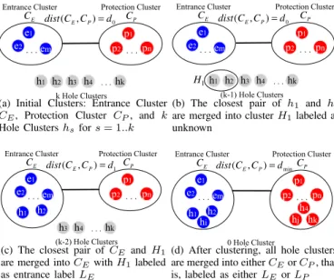
set of protection points. LetLE be entrance label andLP be pro-tection label. We can label the holes inH, by partitioningH into two disjoint subsets (called clusters) Entrance Cluster (CE) and Protection Cluster (CP). Asano et al. proposed such a clustering algorithm for a farthest k-partition based on Minimum Spanning Tree (MST) [15], giving an optimal clustering to maximize the inter-cluster distance. We extend Asano’s Clustering for sensing hole labeling.

Figure 11 illustrates the main idea. Let dist(CE, CP) be the inter-cluster distance between CE and CP. Our objective is to partition the set H into two disjoint sets CE and CP such that the inter-cluster distance betweenCE andCP is maximized. The initial inter-cluster distance is dist(CE, CP) = d0, as shown in Figure 11(a). In this example, suppose that two hole clustersh1 and h2 are the closest pair of two clusters. In this case, these

p2 e2 p1 pn . . . e1 em . . . h2 . . .hk k Hole Clusters 0 ) , (C C d dist _E _P = h3 h4

Entrance Cluster Protection Cluster

E

C C_P

h1

(a) Initial Clusters: Entrance Cluster

CE, Protection Cluster CP, and k Hole Clustershsfors= 1..k

(k-1) Hole Clusters e1 e2 _e_m . . . p1 p2 _{. . .}pn 0 ) , (C C d dist E P =

E C CP h2 h3 h4 . . .hk h1 1 H

(b) The closest pair of h1 and h2

are merged into clusterH1labeled as

unknown e1 e2 _e_m . . . h1 h2 1 ) , (C C d dist _E _P =

E C C_P p1 p2 _{. . .} pn hk . . . (k-2) Hole Clusters h3 h4

(c) The closest pair ofCE andH1

are merged intoCEwithH1labeled

as entrance labelLE e1 e2 _e_m . . . p1 p2 _{. . .}pn h1 h2 0 Hole Cluster min ) , (C C d dist E P = h4 hi hj hk

E

C CP

(d) After clustering, all hole clusters are merged into eitherCEorCP, that is, labeled as eitherLE orLP Fig. 11. Clustering for Sensing Hole Labeling

hole clusters are merged into one hole clusterH1with the same, unknown label, as shown in Figure 11(b). The reason two clusters

h1andh2are merged into one hole cluster with the same label is to let the inter-cluster distance betweenCEandCP be maximized. Otherwise, the inter-cluster distance betweenh1andh2can be the inter-cluster distance shorter than the initial inter-cluster distance

dist(CE, CP) =d0. As shown in Figure 11(c), two clusters CE and H1 are the closest pair, so H1 is merged into CE with hole endpoints h1 and h2 labeled as entrance. In this way, we can cluster all of the hole endpoints into eitherCEorCP to maximize the inter-cluster distancedist(CE, CP), as shown in Figure 11(d). Similar to Asano’s algorithm [15], our clustering gives an optimal hole labeling because it satisfies the greedy choice propertyand optimal substructure [12].

As an important difference from Asano’s Clustering, during the clustering, we maintain multiple hole clusters Hi labeled as unknown in addition to one Entrance Cluster CE and one Protection Cluster CP. Through the MST construction, we merge one hole clusterHi to eitherCE orCP such that the inter-cluster distance between CE and CP is maximized. We call this new labeling algorithm the MST-based Labeling.

3.3.2 Sensing Holes due to Energy Depletion or Failure

In the previous section, we discussed the initial sensing hole issue. However, since in reality, the sensors deployed on road network may not have the same amount of energy initially, we need to consider the sensing holes caused by this unbalanced sensor energy budget. Also sensor could fail over time. We can deal with these sensing holes in the same way as with the initial holes; we can either completely relabel all holes or incrementally label new holes by using MST-based Labeling. The former is optimal, but the latter introduces less computation.

To detect the failure of sensors due to energy depletion, the sensors can regularly report their existence to VISA Scheduler. Also, in a distributed way, the neighboring nodes can exchange their health status with each other in a regular basis. We leave this kind of fault node detection as future work, because inVISA, the fault node detection is not a key design component.

(8)

3.4 Handling of Detection Failure Probability

In reality, there exist sensing errors in sensors. We need to relax the assumption that every vehicle within the sensing range of some sensors can be detected with probability one. Letp be the probability of a success (called detection success probability) on each sensing for working time w. When the required network-wide detection probability for mobile targets is given asPreq(e.g., 0.99) and the sensor’s detection success probability is known as

p = 0.9, the question is how to schedule sensors in order to achieve the user-required detection probabilityPreq. The idea is to perform multiple sensing activities. For example, let q be the probability of a failure (calleddetection failure probability) where

q= 1−p. When p= 0.9,q= 0.1, which means that there exists one detection missing among ten detection trials. LetPreq = 0.99, which means that there exists one detection missing among one hundred detection trials. Assume that a mobile target is staying at a sensor’s sensing range. In order to achievePreq= 0.99, the sensor needs to perform two consecutive sensing activities because the corresponding network-wide detection failure probability is 1−Preq = 0.01 and the detection failure of two consecutive sensing activities is (1−q)2 = 0.01. Another way is for two sensors to perform their sensing activity simultaneously for the mobile target. The first approach is defined astemporal redundant sensingand the second asspatial redundant sensing. Our scheme to deal with the detection failure probability is the combination of these two approaches, defined asredundant sensing.

First, we explain the number of redundant sensing activities

N given q and Preq. Let P¯req be the network-wide detection failure probability such thatP¯req= 1−Preq. Suppose the sensing activities are independent and identically distributed (i.i.d.). The numberN can be computed as follows:

qN ≤P¯req⇒N =⌈logqP¯req⌉. (5)

Time [sec] 0 W or k i ng S ch e dul e _T _w work = period T w N nw Tscan= +( −1) Tsilent=l/v−(N−1)w Scan Time Silent Time

1 2 3 ... k ... n-1 n 1 2 3 ... k ... n-1 n 1 2 3 ... k ... n-1 n 1 2 3 ... k ... n-1 n 1 2 3 ... k ... n-1 n 1 2 3 ... k ... n-1 n

Fig. 12. Scheduling Time Diagram for Redundant Sensing

P 1 2 3 4 E n n-1 n-2 . . . Scan Window (a) Scan by Sensor 1

P 1 2 3 4 E n n-1 n-2 . . . Scan Window (b) Scan by Sensors 1 and 2

P 1 2 3 4 Scan Window E n n-1 n-2 . . .

(c) Scan by Sensors 1, 2 and 3

P 1 2 3 4 E n n-1 n-2 . . . Scan Window (d) Scan by Sensors 2, 3 and 4 Fig. 13. Virtual Scanning for Redundant Sensing

Figure 12 shows the scheduling time diagram for the redun-dant sensing in the Virtual Scanning. As shown in the figure, each sensor performs N sensing activities consecutively. For the redundant sensing, we performNvirtual scans consecutively from the protection point towards the entrance point. To guarantee that a mobile target is scanned at leastN times, the silent timeTsilent is reduced to _vl −(N−1)w. This is becauseN scans should be started before the mobile target reaches the protection point.

Figure 13 shows the virtual scanning for the redundant sensing whereN = 3, which is equivalent to the scheduling time diagram in Figure 12. The scan window is defined as the cluster of adjacent working sensors. Initially, as shown in Figure 13(a), when sensor

s1is working, the size of the scan window is 1. After the working timew, as shown in Figure 13(b), the size becomes 2 since two sensorss1ands2are working together. After anotherw, as shown in Figure 13(c), the size becomes 3 since three sensors s1, s2 and s3 are working together. Finally, after another w, as shown in Figure 13(d), the scan window of size 3 is shifted to the left because the numberN of simultaneous working sensors is 3.

For theDuty Cycling, each sensor performsN sensing activities per its duty cycle in order to provide the same detection probability as with theVirtual Scanning. On the other hand, for the Always-Awake, no change is required for the redudant sensing, because it can already provide such a redudant sensing. We summarize the performance analysis for these three approaches in Table 3 in terms of the maximum network lifetime Tnet. Note that the network lifetime is usually less than Tnet since a vehicle can pass the sensor network at any time without detection where each sensor can detect a vehicle with detection success probability p

per sensing trial; that is, because the sensor network tries to detect the vehicle N times with the detection success probabilitypper sensing trial, it can fail detecting the vehicle with probability (1−p)N _for_N _{trials per duty cycle.}

3.5 Handling of Time Synchronization Error

Up to this point, it is assumed that sensors in VISA system are roughly time-synchronized as long as there is no time gap between two neighboring sensors during the scan time for vehicle detection. Considering that many state-of-the-art solutions [6], [7] can provide sensors with the time synchronization at the microsecond level, we explain how to perform the virtual scanning to satisfy this assumption in this subsection.

Figure 14 illustrates the handling of the time synchronization by the overlap of the working schedules through the margin of sensing time. As shown in Figure 14(a), there exist time gaps among the working schedules of sensors sk−1, sk and sk+1. However, as shown in Figure 14(b), through the margin of the working time based on the maximum time synchronization errorǫmax, the working schedules have time overlaps, guaranteeing no time gaps among the working schedules.

This detection guarantee can be explained in a more formal way as follows: Suppose that a maximum time synchronization error is known asǫmax, sensorsk is required to have a margin ofǫmax for its working start timets

kand working end timetek such that the working schedule is[ts

k−ǫmax, tek+ǫmax]. This allows two adja-cent sensors’ working schedules to overlap even under maximum time synchronization errors. It can be explained that this working

(9)

TABLE 3

Performance Analysis for Three Approaches in Redudant Sensing

Approach Sleeping (Tsleep) Working (Twork) Maximum Network Lifetime (Tnet)

Always-Awake 0 Tlif e Tlif e

Duty Cycling _vl−(N−1)w N w ⌊Tlif e

N w ⌋(N w+ l v−(N−1)w) Virtual Scanning (n−1)w+ l v−(N−1)w N w ⌊ Tlif e N w ⌋(nw+ l v) Time W o rk in g S ch ed u le k

...

k-1 k+1

...

time gap s k t −1 e k t −1 s k t e k t s k t +1 e k t +1 time gap

(a) Scheduling Time Diagram with Time Gap

Time W o rk in g S ch ed u le

...

time overlap max ε − s k t +εmax e k t k-1 k k+1 time overlap max 1+ε − e k t +1−εmax s k t

(b) Scheduling Time Diagram with Time Overlap Fig. 14. Handling of Time Synchronization Error

schedule with a margin ofǫmaxguarantees the target detection as follows: Suppose that the working time isw, the accurate working schedules of two adjacent sensorsskandsk+1are[t∗, t∗+w]and [t∗₊_{w, t}∗_{+ 2}_w_{], respectively, and the their synchronization errors} are ǫk and ǫk+1 ∈ [−ǫmax, ǫmax], respectively. Let us consider the worst scenario for the maximum time gap between these two working schedules, that is, ǫk =−ǫmax andǫk+1 =ǫmax. This setting makes the following working schedules: (i) sk’s working schedule = [t∗₋_ǫ

max, t∗ +w−ǫmax] and (ii) sk+1’s working schedule =[t∗₊_w₊_ǫ

max, t∗+2w+ǫmax]. Now, we augment these two schedules with the maximum time synchronization errorǫmax for the safe detection as follows: (i) sk’s new working schedule = [t∗₋₂_ǫ

max, t∗+w] and (ii) sk+1’s new working schedule = [t∗₊_{w, t}∗_{+ 2}_w_{+ 2}_ǫ

max].Thus, these new working schedules have no time gap, so the targets can be detected without missing. Note the sleeping time Tsleep for sensor sk decreases by 2ǫmax since the working timeTworkbecomesw+2ǫmaxin the schedule period

Tperiod.Duty Cyclingalso needs to adjust each sensor’s working

time and sleeping time by w+ 2ǫmax in the same way as with

Virtual Scanning. On the other hand,Always-Awakedoes not need this adjustment since it does not have any sleeping time.

4 PERFORMANCE

EVALUATION

In this section, we analyze performance of VISA, comparing with other schemes for road network surveillance.

• Performance Metrics:We usenetwork lifetimeandaverage

detection timeas the performance metrics.

• Baselines: Since the road network surveillance is a new

research area, to the best of our knowledge, there exist no other state-of-the-art sensing schemes for road network surveillance. We compare VISA with two approaches: Duty CyclingandAlways-Awake.

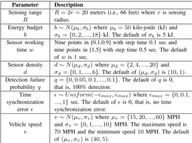
• Parameters:In the performance comparison, we investigate

the effect of the following three parameters: (i) working time, (ii) sensor density, (iii) time synchronization error, and (iv) detection failure probability. In addition, we reveal (i) the effect of sleeping time duration and (ii) the effect of sensing hole labeling.

Simulation uses the map of a real road network as shown in Figure 7. For vehicle mobility, vehicles arrive at the specified entrances of the road network and randomly choose one protection point as destination, moving towards the destination via the shortest path. The vehicle arrival time is uniformly distributed during the system lifetime with mean inter-arrival time 60 sec. The system parameters are selected based on a typical military scenario [16]. Unless mentioned otherwise, the default values in Table 4 are used. Based on these settings, we implemented our own event-driven simulator for evaluation.

TABLE 4

Simulation Configuration

Parameter Description

Sensing range R= 2r= 20meters (i.e., 66 feet) whereris sensing

R radius.

Energy budget b∼N(µb, σb)whereµb= 50kilo-joule (kJ) and

b σb={0,2, ...,18}kJ. The default ofσbis 5 kJ. Sensor working Nine points in [0.1,0.9] with step time 0.1 sec and

timew nine points in [1,5] with step time 0.5 sec. The default ofwis 1 sec.

Sensor density d∼N(µd, σd)whereµd={2,4, ...,20}and

d σd={0,1, ...,6}. The default of(µd, σd)is(10,1). Detection failure q={0,0.05,0.1, ...,0.1}. The default ofqis 0,

probabilityq that is, 100% detection.

Time ǫ∼U nif orm(−ǫmax, ǫmax)whereǫmax={0,0.1, synchronization ...,1}sec. The default ofǫis 0, that is, no time

errorǫ synchronization error.

v∼N(µv, σv)whereµv={15,20, ...,60}MPH Vehicle speed andσv={0,1, ...,10}MPH. The maximum speed is

v 70MPH and the minimum speed10MPH. The default

of(µv, σv)is(40,5).

For network lifetime measurement, the default energy budget (50 kJ) is used, but for the average detection time measurement, to obtain high statistical confidence, a full-day energy budget is used for the comparison among the three approaches.

4.1 System Behavior over Time

All three methods Virtual Scanning,Duty Cycling and Always-Awake can guarantee the detection of targets. Their difference lies in the network lifetime. Clearly, as a node can sleep longer per period with detection guarantee, the more energy efficiency can be obtained. Figure 15 shows how the sleeping time Tsleep changes before network lifetime ends. As shown in the figure, Virtual Scanninghas by far the longest sleeping time and hence the longest network lifetime. For example, Virtual Scanningsustains

(10)

for 28.2 hours, compared with 1.4 hours in Duty Cycling and 5.4 minutes in Always-Awake. This is because of the significant energy savings during the scanning process. Note that in Figure 15, Virtual Scanning lets the sleeping time degrade gradually. This is because as the sensors are dying over time due to energy depletion, the sensing holes occur. These sensing holes let the distance between the entrance cluster and the protection cluster get shorter, as discussed in Section 3.3. Thus, the shorter inter-cluster distance leads to the shorter sleeping time. In the following subsections, we will quantitatively show the effect of the sleeping time on the performance.

0 50 100 150 200 250 300 0 5 10 15 20 25 30

Sleeping Time [sec]

Time [hours]

Virtual Scan Duty Cycling Always-Awake

Fig. 15. The Comparison of Sleeping TimeTsleepover Time

4.2 Performance Comparison

In this section, we compare three approaches: (i)Virtual Scanning, (ii) Duty Cycling and (iii) Always-Awake in terms of Network Lifetime and Average Detection Time under several user-level parameters, such as working time duration, energy budget, and sensor density. Each point in each experiment is the mean of the results obtained with 10 different random seeds.

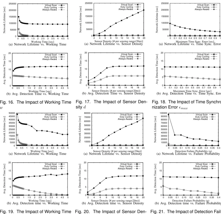
4.2.1 The Impact of Working Time

Since w is the minimum working time before reliable detection can be reported, this evaluation reveals how different hardware response speeds and sensing algorithms affect the VISA and other baselines. We use non-uniform 50kJ energy budget with the energy variation 5kJ. Clearly, VISA provides significantly longer system lifetime than the baselines, especially when w is large as shown in Figure 16(a). For example, whenwis 1 second, VISA extends network lifetime by 18.5 times, compared withDuty Cyclingand 146 times, compared withAlways-Awake. As shown Figure 16(b), the average detection time of Virtual Scanning is 11.5 sec, which is two times longer than that ofDuty Cycling, 5.8 sec. Therefore,Virtual Scanningcan provide 19 times lifetime of Duty Cyclingat the expense of two times longer average detection time.

4.2.2 The Impact of Sensor Density

We definesensor densityas the average number of sensors within sensing range R. As expected from the formula of the network lifetime in Eq. 2, the high sensor density provides the longer network lifetime forVirtual Scanning, as shown in Figure 17(a). This is because with a higher density, we have a longer scanning timeTscan, which allows sensor nodes to sleep longer. However, the high sensor density does not contribute much to the network lifetime to Duty Cyclingand Always-Awake, since their sleeping

time is independent of the number of sensors (as shown in Table 2).

For the average detection time, in both Virtual Scanningand Duty Cycling, under sparse sensor density less than 8, the lower density lets the sensors close to entrances detect vehicles earlier, leading to the shorter average detection time, as shown in Fig-ure 17(b). This is because for initial sensing holes due to low sensor density, the corresponding hole endpoints are labeled as entrance points or protection points for the sensing hole handling discussed in Section 3.3. As the sensor density becomes lower, the distance between the entrance cluster and the protection cluster is getting shorter, leading to the shorter average detection time according to Avg. Detection Time equations in Table 2. On the other hand, under sensor density greater than 8, since the distance between the entrance cluster and the protection cluster is constant regardless of the sensor density, the average detection time is almost the same. In summary, at all sensor density settings,Virtual Scanning provides the longest network lifetime with a small degradation in detection time (e.g., double detection latency), compared with the lifetime increase (e.g., 19 times) where sensor density is 10 with w = 1 sec; note that this performance gain becomes higher when sensor density becomes higher.

4.2.3 The Impact of Time Synchronization Error

We investigate the impact of the time synchronization error on the network lifetime and average detection time. For this investigation, the margin of working time is set to the maximum time synchronization errorǫmax for the safe detection. As shown in Figure 18(a), asǫmax increases, the network lifetimes of both

Virtual ScanningandDuty Cyclingdecrease. This is because each sensor’s working time increases by 2ǫmax and its sleeping time decreases by 2ǫmax, as discussed in Section 3.5.

For the average detection time, as shown in Figure 18(b),Virtual Scanninghas almost the same average detection time regardless of

ǫmax. This is because the average detection time is independent of the working time changed by ǫmax, as shown in Table 2. On the other hand, the average detection time ofDuty Scanningtends to decrease asǫmaxincreases. This is because the average detection time is inversely proportional to the working time increased by 2ǫmax, as shown in Table 2.

4.2.4 The Impact of Detection Failure Probability

In this subsection, we investigate the impact of detection failure probabilityqalong with the following two parameters: (i) working time wand (ii) sensor density d. Figure 19 shows the impact of the working time on the performance in the redundant sensing to deal with the detection failure probability. In the simulation setting, the number of redundant sensing activities is 3 because

q is set to 0.1; that is, since the working time in the redundant sensing is 3 times longer than that in the non-redundant sensing in Section 4.2.1, the lifetime in the redundant sensing is at most one third of that in the non-redundant sensing; note that this maximum lifetime is possible only when vehicles can be detected until the energy budgets of the sensors are depleted completely.

As shown in Figure 19(a), forVirtual Scanning, this expectation is valid when the working time is short, such as from 0.1 to 1 sec; this is caused by the fact that in a short working

(11)

0 50000 100000 150000 200000 250000 0 0.5 1 1.5 2 2.5 3 3.5 4 4.5 5

Network Lifetime [sec]

Working Time [sec]

(a) Network Lifetime vs. Working Time

0 5 10 15 20 0 0.5 1 1.5 2 2.5 3 3.5 4 4.5 5

Working Time [sec]

(b) Avg. Detection Time vs. Working Time Fig. 16. The Impact of Working Time w 0 50000 100000 150000 200000 250000 2 4 6 8 10 12 14 16 18 20

Sensor Density [# per sensing range(20m)]

(a) Network Lifetime vs. Sensor Density

0 5 10 15 20 2 4 6 8 10 12 14 16 18 20

(b) Avg. Detection Time vs. Sensor Density Fig. 17. The Impact of Sensor Den-sityd 0 50000 100000 150000 200000 250000 0 0.1 0.2 0.3 0.4 0.5 0.6 0.7 0.8 0.9 1

Maximum Time Sync. Error [sec]

(a) Network Lifetime vs. Time Sync. Error

0 5 10 15 20 0 0.1 0.2 0.3 0.4 0.5 0.6 0.7 0.8 0.9 1

Maximum Time Sync. Error [sec]

(b) Avg. Detection Time vs. Time Sync. Error Fig. 18. The Impact of Time

Synchro-nization Errorǫmax

0 5000 10000 15000 20000 25000 30000 35000 40000 45000 50000 0 0.5 1 1.5 2 2.5 3 3.5 4 4.5 5

Working Time [sec]

0 5 10 15 20 0 0.5 1 1.5 2 2.5 3 3.5 4 4.5 5

Working Time [sec]

(b) Avg. Detection time vs. Working Time Fig. 19. The Impact of Working Time

wunder Redundant Sensing

0 10000 20000 30000 40000 50000 60000 70000 80000 2 4 6 8 10 12 14 16 18 20

(a) Network Lifetime vs. Sensor Density

0 5 10 15 20 2 4 6 8 10 12 14 16 18 20

(b) Avg. Detection time vs. Sensor Density Fig. 20. The Impact of Sensor

Den-sitydunder Redundant Sensing

0 10000 20000 30000 40000 50000 60000 70000 80000 90000 100000 0 0.05 0.1 0.15 0.2 0.25 0.3 0.35 0.4

Detection Failure Probability (q)

(a) Network Lifetime vs. Failure Probability

0 5 10 15 20 0 0.05 0.1 0.15 0.2 0.25 0.3 0.35 0.4

Detection Failure Probability (q)

(b) Avg. Detection time vs. Failure Probability Fig. 21. The Impact of Detection

Fail-ure Probabilityq

time, neighboring sensors can perform more than three sensing activities. For example, suppose that two sensors s1 and s2 are almost in the same location and the working timewis 0.1 sec. For the sensing circle of 20 meters, a vehicle takes almost 1 second to pass this sensing circle with the speed of 40 MPH. These two sensors can try to detect the vehicle 3 times, respectively; the total number of trials becomes 6. Thus, the network-wide detection failure probability is q6_{= 10}−6 _{that is a very small number. On} the other hand, for the working time longer than 1 sec, the lifetime is decreasing because the network-wide detection can fail earlier than the maximum lifetime with only three detection trials; in this case, the network-wide detection failure probability isq3_{= 10}−3_. Thus, the benefit of the spatial redundant sensing decreases as the working time increases. Note that in Figure 19(a), the curve

is not smooth from w = 1 sec to w = 2 sec. After w = 1 sec, the network-wide detection failure probability dramatically increases with less spatial redundant sensing. For Duty Cycling, the lifetime tends to decrease as the working time increases in the similar way with the case of the non-redundant sensing. For

w= 0.1sec,Virtual Scanninghas 2.89 times longer lifetime than Duty Cycling. For the working time longer than0.5 sec, Virtual Scanninghas at least 10 times longer lifetime thanDuty Cycling. As shown in Figure 19(b), the average detection time ofVirtual Scanningincreases slightly as the working time increases. This is because the network-wide detection failure probability increases with less spatial redundant sensing according to the increase of the working time, leading to a little later detection. ForDuty Cycling, the average detection time decreases faster for the increase of the

(12)

working time than that in the non-redundant sensing, as shown in Figure 19(b). This is because the redundant sensing increases the working time per duty cycle; note that the average detection time is inversely proportional to the working time.

For the sensor density, as shown in Figure 20, the patterns of the curves ofVirtual ScanningandDuty Cyclingare similar to those in the non-redundant sensing, as shown in Figure 17. The remarkable difference in the network lifetime is that the lifetimes ofVirtual ScanningandDuty Cycling are reduced to almost one third. For the average detection time,Virtual Scanninghas almost the same detection time as with the case of the non-redundant sensing. The average detection time of Duty Cycling is shorter than the case of the non-redundant sensing. This is because that the average detection time is inversely proportional to the working time and the working time is increased due to the redundant sensing.

Now, we investigate the impact of detection failure probabil-ity on both peformance metrics. For the lifetime, as shown in Figure 21(a), Virtual Scanninghas shorter lifetime according to the increase of detection failure probability q, leading to the increasing number of sensing activities per duty cycle. However, the performance gain ofVirtual Scanningin the lifetime is at least 17 times over Duty Cycling and at least 20 times over Always-Awake. For the average detection time, as shown in Figure 21(b), Virtual Scanninghas almost the constant detection time, however Duty Cyclingtends to have a shorter detection time according to the increase of q; this is because the increase of q leads to the increase of the working time.

In summary, even in the realistic setting with the time synchro-nization error and detection failure probability, Virtual Scanning outperforms both Duty Cycling and Always-Awake in terms of network lifetime.

4.3 Achieving Shorter Delay and Longer Lifetime Simul-taneously

In this subsection, we show that there exists a working time such thatVirtual Scanningis better in both the detection delay and the lifetime thanDuty Cycling. In Section 2.4, we showed analytically how VISA achieves a shorter delay and a longer network lifetime simultaneously by adjusting thesilent time (Tsilent =α) within the range that satisfies Eq. 3 where the silent time is part of the sleeping time. To confirm our design empirically, Figure 22 shows the performance effect of Virtual Scanning according to α. As shown in Figure 22, whenVirtual ScanningreducesαfromTsilent to0in the working time of0.1 second, it has better performance in both the network lifetime and average detection time thanDuty Cycling. Therefore, the system operator can achieve the required performance by tuning the working time and the sleeping time.

4.4 The Effect of Hole Handling

This section compares three different methods for hole handling: • MST-based Labeling: our hole labeling scheme discussed in

Section 3.3.

• Random Labeling: a new hole is randomly labeled as either pseudoentrance point orpseudoprotection point.

• No Labeling: when a new hole occurs, it is not handled, leading to the end of system lifetime.

0 50000 100000 150000 200000 250000 0 0.5 1 1.5 2 2.5 3 3.5 4 4.5 5

Working Time [sec] Virtual Scan with α=Tsilent Virtual Scan with α=Tsilent/2 Virtual Scan with α=0 Duty Cycling

0 5 10 15 20 0 0.5 1 1.5 2 2.5 3 3.5 4 4.5 5

Working Time [sec] Virtual Scan with α=Tsilent Virtual Scan with α=Tsilent/2 Virtual Scan with α=0 Duty Cycling

(b) Avg. Detection time vs. Working Time

Fig. 22. The Impact of Silent Timeα

0 50000 100000 150000 200000 250000 0 0.5 1 1.5 2 2.5 3 3.5 4 4.5 5

Working Time [sec] MST-based Labeling

Random Labeling No Labeling

Fig. 23. The Comparison of Hole Labeling Algorithms

We use the same Virtual Scanning for these three labeling algorithms. As shown in Figure 23, MST-based Labeling gives longer lifetime than both Random Labeling and No Labeling. Random Labeling and No Labeling have the similar lifetime, because Random Labeling cannot label holes appropriately to prevent a breach path (i.e., path vulnerable to vehicle intrusion to protection points) from existing; that is, since Random Label-ing might label holes against our labeling rule based on MST discussed in Section 3.3.1 (i.e., to label two closest holes with the same label for longer lifetime), the holes close to entrance points can have different labels, leading to the short sleeping time. Since No Labelingdoes not handle sensing hole, one sensing hole creates a breach path, leading to the end of system.

For the average detection time, these three labeling algorithms have similar performance whose curves are almost the same as the curve of Virtual Scanningin Figure 16(b).

5 WORK

Most research on coverage for detection has so far focused on Full Coverage[1]–[4], [17]–[20] in a 2-dimensional space. In [4], authors use the off-duty eligibility rule to turn on/off a node as long as the neighboring nodes can cover the sensing area of this node. The Coverage Configuration Protocol (CCP) [18] provides an energy-efficient sensing coverage, integrated with SPAN for connectivity. In [21], surveillance coverage is achieved through probing. DiffSurv [22] provides differentiated surveillance to an