HAL Id: hal-01405322
https://hal.inria.fr/hal-01405322
Submitted on 16 Dec 2016HAL is a multi-disciplinary open access archive for the deposit and dissemination of sci-entific research documents, whether they are pub-lished or not. The documents may come from
L’archive ouverte pluridisciplinaire HAL, est destinée au dépôt et à la diffusion de documents scientifiques de niveau recherche, publiés ou non, émanant des établissements d’enseignement et de
A Cartesian Scheme for Compressible Multimaterial
Models in 3D
Alexia de Brauer, Angelo Iollo, Thomas Milcent
To cite this version:
Alexia de Brauer, Angelo Iollo, Thomas Milcent. A Cartesian Scheme for Compressible Mul-timaterial Models in 3D. Journal of Computational Physics, Elsevier, 2016, 313, pp.121-143. �10.1016/j.jcp.2016.02.032�. �hal-01405322�
A Cartesian Scheme for Compressible
Multimaterial Models in 3D
Alexia de Brauer, Angelo Iollo
∗
Univ. Bordeaux, IMB, UMR 5251, F-33400 Talence, France. CNRS, IMB, UMR 5251, F-33400 Talence, France. INRIA, F-33400 Talence, France.
Thomas Milcent
Univ. Bordeaux, I2M, UMR 5295, F-33400 Talence, France. Arts et M´etiers Paristech, F-33607 Pessac, France.
Abstract
We model the three-dimensional interaction of compressible materials separated by sharp interfaces. We simulate fluid and hyperelastic solid flows in a fully Eu-lerian framework. The scheme is the same for all materials and can handle large deformations and frictionless contacts. Necessary conditions for hyperbolicity of the hyperelastic neohookean model in three dimensions are proved thanks to an explicit computation of the characteristic speeds. We present stiff multimaterial interactions including air-helium and water-air shock interactions, projectile-shield impacts in air and rebounds.
Key words: compressible multimaterial, immersed boundary, Eulerian elasticity
∗ Corresponding author
Email addresses: [email protected] (Alexia de Brauer),[email protected] (Angelo Iollo),
1 Introduction
The study of three-dimensional multimaterial phenomena requires efficient nu-merical modeling and simulation. These problems are insoluble by traditional theoretical and experimental approaches and hazardous to study in the labo-ratory. Nevertheless, their accurate and efficient simulation is crucial to reduce environmental impact in many industrial domains. Numerical model research in this field is particularly active because of the formidable difficulty in apply-ing classical approaches based onad hoc models and schemes to multi-physics contexts.
In what follows we focus on phenomena that involve gases, liquids and elastic materials undergoing rapid evolution and large deformations in three space dimensions. For this reason, we privilege a fully Eulerian approach and a monolithic model that describes each material by the same set of conservation equations and an appropriate thermodynamically consistent constitutive law different for each material [15]. For specific applications, typically in presence of mostly radial phenomena, Lagrangian or Lagrangian-Eulerian approaches may be more pertinent, see [20,13,6,21].
Fully Eulerian hyperbolic conservative models for continuum mechanics were introduced in [15,26,27] and their numerical analysis started in [12,24]. In [12] the authors propose a scheme, the ghost-fluid method, that allows an implicit capturing of the material interfaces. Moreover, they devise a locally non-conservative Godunov solver at the interface that is stable and non oscil-latory. This scheme relies on the definition of a ghost medium that requires the storage of additional variables at the material interfaces, where the solution of two Riemann problems, each relative to a different material, is necessary. A different method was proposed in [24] where a conservative cut-cell tech-nique was developed for hyperelastic and plastic multimaterial simulations. A specific feature of this numerical model is that the deviations of the deforma-tion gradient with respect to the irrotadeforma-tional compatibility condideforma-tion and to continuity equation are explicitly penalized in the governing equations. This scheme is at the base of many other subsequent works in the literature. Another approach is introduced in [11] for hyperelastic solid and fluid
interac-tions. The authors design a conservative non-equilibrium mixture model that relaxes to the desired multimaterial conservation laws. In this approach one compromises on the sharpness of the material interface to avoid oscillations and to apply an HLLC solver previously developed for a single material in [14]. Further developments of this method include plasticity modeling [10] and an hyperbolic sub-system splitting procedure [9] where each sub-system has only three waves instead of seven.
The analysis and the simulation of three-dimensional hyperelastic models present specific difficulties due to the seven-wave pattern and to the inher-ent hyperbolicity constraint. In [4] an approximation of the Riemann problem based on characteristic tracing is employed to simulate the one-dimensional projection of the seven-wave pattern typical of a three-dimensional hypere-lastic constitutive law. This approach has further been developed in [3] to deal with actual multimaterial interfaces thanks to a variant of the ghost-fluid method, with applications to one-dimensional as well as two-dimensional deformations of multiple hyperelastic sliding materials. A fully conservative cut-cell three-dimensional Eulerian method is then presented in [5] for simu-lating multiple compressible solid and fluid components where internal bound-aries are tracked using level set functions. A different discretization scheme is adopted in [17], where the simulation of elastic and plastic two-dimensional flows is based on a hybrid centered-difference WENO method and a ghost-fluid approach at the interface. The authors employ a fourth-order centered-difference stencil away from discontinuities that requires no explicit calculation of the local hyperbolic characteristic information. As a result, the scheme is constructed in a general way to allow for possibly different constitutive re-lations. In the same spirit, a conventional third-order WENO scheme and a ghost-fluid method are applied in [2] to actual three-dimensional simulations of hyperelastic and plastic impacts and penetration with adaptive mesh refine-ment. It is known that approximate Riemann solvers for such problems may lead to inaccurate intermediate states as noted in [23,4]. However, these local inaccuracies do not seem to significantly pollute the solution when compared to exact test cases [14,11,16].
Hence, the typical features of integration schemes for Eulerian formulations of the hyperelastic conservation laws are: i) tracking of internal boundaries by a level set function; ii) approximate Riemann solver to compute numerical
fluxes; iii) ghost-material approach to compute numerical fluxes at the ma-terial interface. In this respect, the present study details a twofold contribu-tion to the simulacontribu-tion of complex three-dimensional hyperelastic phenomena. Firstly, we show under usual assumptions that the hyperelastic neohookean model employed satisfies the necessary conditions for hyperbolicity by explic-itly computing the analytic wave speeds of small perturbations. Secondly, we simplify the computations of the numerical fluxes at the material interface such that no ghost material is defined and no mixture model is needed to ob-tain a non-oscillatory scheme, extending to three space dimensions the method presented in [16]. Thanks to this method, we are able to explicitly determine the internal boundary conditions modeling shock-bubble interactions, three-dimensional impacts and rebounds of hyperelastic materials immersed in a fluid.
2 The model
This model was already discussed in [15,26,27,24,7,11]. We follow here the formulation presented in [16] where a neohookean model was investigated and extend it to three dimensions.
2.1 Forward and backward characteristics
Let Ω0 ⊂R3 be the reference (or initial) configuration of a continuous medium and Ωt ⊂ R3 the deformed configuration at time t. In order to describe the
evolution of this medium in the Lagrangian frame we define the forward char-acteristicsX(ξ, t) as the image at timetin the deformed configuration of a ma-terial pointξ belonging to the initial configuration, i.e.,X : Ω0×[0, T]−→Ωt,
(ξ, t)7→X(ξ, t) (see Fig.1). The corresponding Eulerian velocity fielduis de-fined asu: Ωt×[0, T]−→R3, (x, t)7→u(x, t) where Xt(ξ, t) =u(X(ξ, t), t) X(ξ,0) =ξ (1)
backward characteristicsY(x, t) (see [7]) that for a timet and a pointxin the deformed configuration, gives the corresponding initial point ξ in the initial configuration, i.e., Y : Ωt×[0, T]−→ Ω0, (x, t) 7→ Y(x, t) (see Fig. 1). Since
Y(X(ξ, t), t) = ξ, differentiating with respect to time and space in turn we have: Yt+u· ∇xY = 0 Y(x,0) =x (2) and [∇ξX(ξ, t)] = [∇xY(x, t)]−1. (3)
The relation (2) is the Eulerian equivalent of the characteristic equation (1). In addition, equation (3) allows to compute the gradient of the deformation in the Eulerian frame via Y.
Y(x, t) =ξ
x=X(ξ, t)
Initial configuration Ω0 Deformed configuration Ωt
Fig. 1. Forward and backward characteristics.
2.2 Eulerian model
The local form of the governing equations of mass, momentum and energy conservation in the deformed configuration Ωt can be written as
ρt+ divx(ρu) = 0
(ρu)t+ divx(ρu⊗u−σ) = 0
(ρe)t+ divx(ρeu−σTu) = 0
(4)
The physical variables are the density ρ(x, t), the velocity u(x, t), the total energy per unit mass e(x, t) and the Cauchy stress tensor in the physical domain σ(x, t). To close these systems a constitutive law is needed to detail the relationship between the stress tensors and the other physical variables.
2.3 Hyperelastic models
The classical results of this section can be found in the textbook [18]. Let us define ε = e− 1
2|u|
2 the internal energy per unit mass. In the hyperelastic context, ε is a function of the deformation tensor ∇ξX and the entropy s.
The energy has to be Galilean invariant and we focus in this paper on the isotropic case. It can be proved that the material is Galilean invariant and isotropic if, and only if, ε is expressed as a function of the invariants of the right Cauchy-Green tensor C(ξ, t) = [∇ξX]T[∇ξX] or equivalently of the
in-variants of the left Cauchy-Green tensorB(ξ, t) = [∇ξX][∇ξX]T. The three
di-mensional invariants often considered in the literature are Tr(·), Tr(Cof(·)) = (Tr(·)2−Tr(·2))/2 and Det(·).
We assume that ε is the sum of εvol, a term depending on volume variation and entropy, and εiso a term accounting for isochoric deformation. Hence the internal energy is given by
ε=εvol(ρ, s) +εiso(Tr(B),Tr(B
−1
)) (5)
where in three dimensions we have
B(x, t) = [∇xY]−1[∇xY]−T/J
2
3(x, t) J(x, t) = det([∇
xY])−1 (6)
the term relative to an isochoric transformation may also depend on entropy. Here, we will limit the discussion to materials where the isochoric term is in-dependent of the entropy, as in the case of idealized crystals (metals, ceramic). The Cauchy stress tensor σ(x, t) is then given by (see [18] for the details)
σ(x, t) =−ρ2∂εvol ∂ρ s (ρ, s)I+ 2J−1 σiso− Tr(σiso) 3 I ! (7) where σiso = ∂εiso ∂α B− ∂εiso ∂β B −1 (8)
and α, β denote the first and second argument of εiso, respectively.
2.4 Overall model
Together with equations of mass, momentum and energy conservation (4), the additional equation (2) is required in order to record the deformation in the Eulerian frame. However, since σ will directly depend on ∇xY (5-7) we
take the gradient of (2) as a governing equation and obtain the system in conservative form ρt+ divx(ρu) = 0
(ρu)t+ divx(ρu⊗u−σ) = 0
(∇xY)t+∇x(u· ∇xY) = 0
(ρe)t+ divx(ρeu−σTu) = 0
(9)
where some fluxes of ∇xY are zero (see equation (13)). The initial
den-sity ρ(x,0), the initial velocity u(x,0), the initial total energy e(x,0) and ∇xY(x,0) = I are given together with appropriate boundary conditions. This
system is known in the literature as the inverse deformation gradient formu-lation.
We choose a general constitutive law that models gas, fluids and elastic solids. The internal energy per unit mass ε=e− 1
2|u|
2 is defined as
ε(ρ, s,∇xY) =
neohookean elastic solid
z }| { κ(s) γ−1 1 ρ −b !1−γ −aρ | {z }
van der Waals gas
+p∞ ρ | {z } stiffened gas +χ ρ0 (Tr(B)−3) (10)
where B is defined in (6). We obtain according to (7)
σ(ρ, s,∇xY) = −p(ρ, s)I+ 2χJ−1 B− Tr(B) 3 I ! (11) where p(ρ, s) = −p∞−aρ2+κ(s) 1 ρ −b !−γ (12) Hereκ(s) = exp s cv
and cv, γ,p∞, a, b, χ are positive constants that
char-acterize a given material. Parametersaandbcorrespond to the van der Waals parameters,p∞accounts for fluid or solid materials where intermolecular forces
are present (see for example [14,11]). The last term in the energy expression models a neohookean elastic solid where the constant χ is the shear elastic modulus. For very large deformations, more complete models (Mooney-Rivlin, Ogden) take into account an additional invariant in the energy function in three dimensions. Without loosing in generality, here we stick to a neohookean model as it leads to simpler expressions in the following developments.
3 Numerical Scheme
Let x = (x1, x2, x3) be the coordinates in the canonical basis of R3, u = (u1, u2, u3) the velocity components, Y,ji the components of the tensor [∇xY]
ρ ρu1 ρu2 ρu3 Y1 ,1 Y2 ,1 Y3 ,1 Y1 ,2 Y2 ,2 Y3 ,2 Y,13 Y2 ,3 Y3 ,3 ρe ,t + ρu1 (ρu1)2 ρ −σ 11 ρu1ρu2 ρ −σ 21 ρu1ρu3 ρ −σ 31
ρu1Y,11+ρu2Y,12+ρu3Y,13
ρ
ρu1Y,21+ρu2Y,22+ρu3Y,23 ρ
ρu1Y,31+ρu2Y,32+ρu3Y,33
ρ 0 0 0 0 0 0
ρu1ρe−(σ11ρu1+σ21ρu2+σ31ρu3)
ρ ,1 + ρu2 ρu1ρu2 ρ −σ 12 (ρu2)2 ρ −σ 22 ρu2ρu3 ρ −σ 32 0 0 0
ρu1Y,11+ρu2Y,12+ρu3Y,13
ρ
ρu1Y,21+ρu2Y,22+ρu3Y,23 ρ
ρu1Y,31+ρu2Y,32+ρu3Y,33
ρ 0
0
0
ρu2ρe−(σ12ρu1+σ22ρu2+σ32ρu3)
ρ ,2 + ρu3 ρu1ρu3 ρ −σ 13 ρu2ρu3 ρ −σ 23 (ρu3)2 ρ −σ 33 0 0 0 0 0 0
ρu1Y,11+ρu2Y,12+ρu3Y,13
ρ
ρu1Y,21+ρu2Y,22+ρu3Y,23
ρ
ρu1Y,31+ρu2Y,32+ρu3Y,33
ρ
ρu3ρe−(σ13ρu1+σ23ρu2+σ33ρu3)
ρ ,3 = 0 0 0 0 0 0 0 0 0 0 0 0 0 0 (13) This system can be written in the compact form
Φt+ (G1(Φ)),1+ (G2(Φ)),2+ (G3(Φ)),3 = 0 (14)
We discretize (14) with a finite volume method on a Cartesian mesh. Let ∆xi
be the grid spacing in the xi direction and Ωi,j,k the control volume centered
at the node (i∆x1, j∆x2, k∆x3). The semi-discretization in space of (14) on Ωi,j,k gives (Φi,j,k)t+ G1 i+1/2,j,k−G1i−1/2,j,k ∆x1 +G 2 i,j+1/2,k−G2i,j−1/2,k ∆x2 +G 3 i,j,k+1/2−G3i,j,k−1/2 ∆x3 = 0 (15)
where Φi,j,k is the value of the conservative variable integrated on Ωi,j,k. In
Fig. 2 are shown sections in two dimensions of the three-dimensional compu-tational cell projected on their respective parallel planes.
x y z i∆x1 j∆x2 k∆x3 (i−1)∆x1 (i+ 1)∆x1 (j−1)∆x2 (j+ 1)∆x2 (k−1)∆x3 (k+ 1)∆x3 Φi−1,j,k Φi+1,j,k Φi−1,j,k Φi+1,j,k Φi,j−1,k Φi,j+1,k Φi,j−1,k Φi,j+1,k Φi,j,k−1 Φi,j,k+1 Φi,j,k−1 Φi,j,k+1 G1i−1 2,j,k G1i+1 2,j,k G2 i,j−1 2,k G2 i,j+12,k G3 i,j,k−1 2 G3 i,j,k+12
Φ
i,j,kFig. 2. Discretization on the control volume Ωi,j,k. Two-dimensional sections of the
computational cell are projected on planes (xy), (yz) and (zx).
The fluxes in (15) will be computed by approximate one-dimensional Riemann solvers in the direction orthogonal to the cell sides of the Cartesian mesh. Therefore, we have
G1i−1/2,j,k ≈ F(Φi−1,j,k; Φi,j,k) G1i+1/2,j,k ≈ F(Φi,j,k; Φi+1,j,k) (16)
G2i,j−1/2,k ≈ F(Φi,j−1,k; Φi,j,k) G2i,j+1/2,k ≈ F(Φi,j,k; Φi,j+1,k) (17)
whereF(·; ·) is a numerical flux function that will be specified in the follow-ing.
The fluxes in (13) are the same in the three spatial directions. Let us consider the one-dimensional problem in the x1 direction
Φt+ (G1(Φ)),1 = 0 (19)
where we have (Y,i2)t= (Y,3i)t = 0. These equations introduce six characteristics
in (19) whose speeds are 0. This means also that Y,i2 and Y,i3 are just constant parameters in the other equations of the system. Therefore, in the next sections we focus on the wave structure of the following one-dimensional problem
Ψt+ (F(Ψ)),1 = 0 (20) where Ψ = ρ ρu1 ρu2 ρu3 Y1 ,1 Y2 ,1 Y,13 ρe F(Ψ) = ρu1 (ρu1)2 ρ −σ 11 ρu1ρu2 ρ −σ 21 ρu1ρu3 ρ −σ 31
ρu1Y,11+ρu2Y,12+ρu3Y,13
ρ
ρu1Y,21+ρu2Y,22+ρu3Y,23
ρ
ρu1Y,31+ρu2Y,32+ρu3Y,33
ρ
ρu1ρe−(σ11ρu1+σ21ρu2+σ31ρu3)
ρ . 4 Characteristic speeds
In this section we extend in three dimensions the criterion given in [16] to analytically compute the wave speeds. Also, we prove that when we consider
a neohookean constitutive law, the wave speeds are real for any deformation under usual assumptions.
4.1 General case
The governing equations (20) are closed with the constitutive law (5)-(7) which defines σ as a non-linear function of the unknowns. In this adiabatic and in-viscid model, it can be shown that entropy is just transported along the char-acteristics for smooth solutions. Since the wave velocities are locally defined by infinitesimal smooth variations of the conservative variables Ψ, the energy equation can be simply replaced by st+u· ∇s= 0. Thus, instead of (20), we
study the following quasi-linear system:
ρ ρu1 ρu2 ρu3 Y,11 Y2 ,1 Y3 ,1 s ,t + 0 1 0 0 0 0 0 0 −(ρu1)2 ρ2 2ρu1 ρ 0 0 −σ 11 ,1 −σ,112 −σ,113 −σ,s11 −ρu1ρu2 ρ2 ρu2 ρ ρu1 ρ 0 −σ 21 ,1 −σ,212 −σ,213 −σ,s21 −ρu1ρu3 ρ2 ρu3 ρ 0 ρu1 ρ −σ 31 ,1 −σ,312 −σ,313 −σ,s31
−ρu1Y,11+ρu2Y,12+ρu3Y,13
ρ2 Y1 ,1 ρ Y1 ,2 ρ Y1 ,3 ρ ρu1 ρ 0 0 0
−ρu1Y,21+ρu2Y,22+ρu3Y,23
ρ2 Y2 ,1 ρ Y2 ,1 ρ Y2 ,3 ρ 0 ρu1 ρ 0 0
−ρu1Y,31+ρu2Y,32+ρu3Y,33
ρ2 Y3 ,1 ρ Y3 ,1 ρ Y3 ,3 ρ 0 0 ρu1 ρ 0 0 0 0 0 0 0 0 ρu1 ρ ρ ρu1 ρu2 ρu3 Y,11 Y2 ,1 Y3 ,1 s ,1 = 0 0 0 0 0 0 0 0 (21) whereσij,1,σ,ij2,σij,3, and σij
,s denote the derivative of σij with respect toY,11,Y,12,
Y,31 and s respectively. We denote by Jac the matrix appearing in (21).
Σ = [∇σ][∇Y] := σ11 ,1 σ11,2 σ,113 σ21 ,1 σ21,2 σ,213 σ31,1 σ31,2 σ,313 Y1 ,1 Y,12 Y,31 Y2 ,1 Y,22 Y,32 Y,31 Y,32 Y,33 (22)
The characteristic polynomial of Jac can be written under the form
P(λ) = (λ−u1) 2
ρ3 ((ρ(u1−λ) 2
)3+ Tr(Σ)(ρ(u1−λ)2)2+ Tr(Cof((Σ))(ρ(u1−λ)2) + Det(Σ))
so that the eigenvalues of Jac are
ΛE = ( u1, u1, u1 ± s α1 ρ , u1± s α2 ρ , u1± s α3 ρ ) (23)
where α1, α2 and α3 are the roots of the polynomial of third order
X3+ Tr(Σ)X2+ Tr(Cof((Σ))X+ Det(Σ) = 0 (24)
Therefore, the necessary conditions for system (20) to be hyperbolic are α1 > 0, α2 >0 andα3 >0. In [25] it is shown that these conditions are also sufficient to ensure that a complete system of eigenvectors of the Jacobian matrix exists.
Roots of third order polynomial
With the change of variablesX =Z−Tr(Σ)/3, equation (24) reduces to
Z3+PZ+Q= 0 (25)
P = Tr(Cof((Σ))− Tr(Σ) 2 3 Q= 2Tr(Σ)3 27 − Tr(Σ)Tr(Cof((Σ)) 3 + Det(Σ) (26)
The three solutions are reals if ∆3D = 4P3+ 27Q2 ≤0 (which impliesP ≤0)
and are given by
αk = 2 s −P 3 cos 1 3arccos −sign(Q) s 1−∆3D 4P3 + 2kπ 3 − Tr(Σ) 3 k = 1,2,3 (27)
Moreover, the αi are positive if Tr(Σ) <0,Tr(Cof((Σ))>0 and Det(Σ) <0.
In the particular case where ∆3D = 0 we obtain a solution of multiplicity two
α1 = 3Q P − Tr(Σ) 3 α2 =α3 =− 3Q 2P − Tr(Σ) 3 (28)
4.2 Hyperbolicity of the neohookean model
The internal energy ε with the neohookean model reads
ε=εiso(ρ, s) + χ ρ0 (Tr(B)−3) (29) LetA be Aij = (−1)i+j(K1iK1j+K2iK2j+K3iK3j) (30) where
K11=Y,22Y,33−Y,23Y,23 K21 =Y,21Y,33−Y,23Y,13 K31=Y,12Y,23−Y,22Y,31 K12=Y,21Y 3 ,3−Y 3 ,1Y 2 ,3 K22 =Y,11Y 3 ,3 −Y 3 ,1Y 1 ,3 K32=Y,11Y 2 ,3−Y 2 ,1Y 1 ,3 K13=Y,21Y 3 ,2−Y 3 ,1Y 2 ,2 K23 =Y,11Y 3 ,2 −Y 3 ,1Y 1 ,2 K33=Y,11Y 2 ,2−Y 2 ,1Y 1 ,2
We can show thatJ−1B =AJ13. Therefore the expression of the stress tensorσ
(11) becomes
σ =−p(ρ, s)I+ 2χJ13 A− Tr(A)
3 I
!
(31)
Using the square of the sound speed c2(ρ, s) = ∂p ∂ρ s, (22) changes into Σ = 2 9χJ 1/3 D1 D2J β2+ 6A12 D2J β3+ 6A13 6A12 −3β2J A12−9A11 −3β3J A12 6A13 −3β2J A13 −3β3J A13−9A11 −ρc2 1 0 0 0 0 0 0 0 0 (32) where D1 =−2A11−5A22−5A33 D2 =−2A11+A22+A33 β2 =K11Y,21−K21Y,22+K31Y,32 β3 =K11Y,13−K21Y,23 +K31Y,33
and we have the relation β2A12+β3A13 = 0 Thus, it follows that
Tr(Σ) =− ρc2+10 9χJ 1 3(4A 11+A22+A33) (33) Tr(Cof(Σ)) = 4χJ13 A11ρc2+ 1 9χJ 1 3(C1+ 11A2 11+ 5A11(A22+A33)) (34) det(Σ) =−(2χJ13)2A11 A11ρc2+ 2 9χJ 1 3C1 (35) where C1 = 2A211+ (A12)2+ (A13)2+ 5(A11A22−(A12)2+A11A33−(A13)2)
We have that C1 ≥0 because
A11A22−(A12)2 = (K12K21−K11K22)2+ (K12K31−K11K32)2+ (K22K31−K21K32)2 ≥0
A11A33−(A13)2 = (K13K21−K11K23)2+ (K13K31−K11K33)2+ (K23K31−K21K33)2 ≥0
Since Aii ≥ 0, it follows that Tr(Σ) ≤ 0,Tr(Cof((Σ)) > 0 and Det(Σ) < 0.
The reduced parameters are then given by
P =−1 3 ρc2− 2 9χJ 1 3C2 2 + 4 3(2χJ 1 3)2C3 ! (36) Q=− 2 27 ρc2− 2 9χJ 1 3C 2 ρc2−2 9χJ 1 3C 2 2 + 2(2χJ13)2C 3 ! (37) ∆3D =− 1 9 4 3(2χJ 1 3)2C3 2 ρc2− 2 9χJ 1 3C2 2 +16 9 (2χJ 1 3)2C3 ! (38) where C2 = 7A11−5(A22+A33) C3 = (A12)2+ (A13)2 ≥0
As C3 ≥0 we obtain that P ≤0 and ∆3D ≤0. Also, the sign of Qis equal to
the sign of 29χJ13C2−ρc2.
This result shows that the necessary conditions for the neohookean model to be hyperbolic are satisfied, since the wave speeds given by (23) and (27) are real for any deformation, under the usual assumptions c2 >0 and χ≥0.
4.3 Small deformations
We investigate the simplifications of the wave speeds for small deformations. In this case∇Y ≈I and Aij =δij. Hence, we have
C1 = 12 C2 = 3 C3 = 0 and (33)-(35) reduce to Tr(Σ) =− ρc2+20 3χ ≤0 Tr(Cof(Σ)) = 4χ ρc2 +11 3 χ ≥0 det(Σ) =−4χ2 ρc2 +8 3χ ≤0
The reduced parameters are given by
P =−1 3 ρc2+ 2 3χ 2 Q=− 2 27 ρc2+2 3χ 3 ∆3D = 0
ΛE = ( u1, u1, u1± s c2+ 4 3 2χ ρ , u1± s 2χ ρ , u1± s 2χ ρ ) (39)
Therefore, in the small deformation limit the speeds corresponding to trans-verse waves coincide, as in the classical theory of linear elasticity.
5 Numerical flux
In this section we first introduce the HLLC solver employed for a single ma-terial. Then we specify the numerical flux for the multimaterial case.
5.1 HLLC Solver
We consider equation (20) with the initial condition
Ψ(x, t= 0) = Ψl if x≤0 Ψr if x >0, (40)
The numerical flux functionF(Ψl; Ψr) at the cell interfacex= 0 is determined
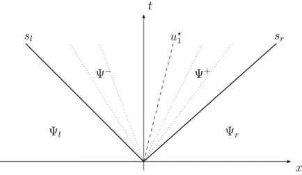
based on the solution of the HLLC [29] approximate Riemann problem, simi-larly to what is done in [14,16]. Even though the exact wave pattern involves seven distinct waves, see (23), the approximate solver approaches the solution using three waves (the contact discontinuityu?
1, the fastest leftward and right-ward wavessl andsr), thus inducing only two intermediate states Ψ− and Ψ+
x t sr u? 1 sl Ψr Ψ+ Ψ− Ψl
Fig. 3. HLLC solver wave pattern.
Let define the intermediate states Ψ− and Ψ+ and their related fluxes as
Ψ−= ρ− ρ−u−1 ρ−u−2 ρ−u−3 (Y1 ,1) − (Y,21)− (Y3 ,1) − (ρe)− F− = ρ−u−1 ρ−(u−1)2−(σ11)? ρ−u−1u−2 −(σ21)? ρ−u−1u−3 −(σ31)? u−1(Y1 ,1) −+u− 2(Y,21) −+u− 3(Y,13) − u−1(Y,21)−+u−2(Y,22)−+u−3(Y,23)− u−1(Y3 ,1) −+u− 2(Y,23) −+u− 3(Y,33) − u−1(ρe)−−((σ11)?u− 1 + (σ21)?u − 2 + (σ31)?u − 3) (41)
Ψ+= ρ+ ρ+u+1 ρ+u+ 2 ρ+u+ 3 (Y,11)+ (Y2 ,1)+ (Y,31)+ (ρe)+ F+ = ρ+u+ 1 ρ+(u+1)2−(σ11)? ρ+u+ 1u+2 −(σ21)? ρ+u+ 1u+3 −(σ31)? u+1(Y,11)++u+2(Y,21)++u+3(Y,13)+ u+1(Y2 ,1)++u + 2(Y,22)++u + 3(Y,23)+ u+1(Y,31)++u+2(Y,23)++u+3(Y,33)+ u+1(ρe)+−((σ11)?u+ 1 + (σ21)?u+2 + (σ31)?u+3) (42)
Here the stresses (σ11)?,(σ21)? and (σ31)? are independent unknowns.
The HLLC scheme is based on the assumption that every wave is a shock and therefore Rankine-Hugoniot relations give
F(Ψr)− F+ =sr(Ψr−Ψ+) F+− F− =u1(Ψ+−Ψ−) F−−F(Ψl) =sl(Ψ−−Ψl) (43)
We introduce the notations
Ql=F(Ψl)−slΨl Qr =F(Ψr)−srΨr (44)
and we denote byQi
l (respectively Qir) thei-th component of Ql (respectively
Qr). In the following, except when otherwise explicitly stated, we take u−1 =
u+1 =u?
1.
ρ−= Q 1 l u−1 −sl ρ+= Q 1 r u+1 −sr (45) (Y,11)−= Q 5 l −u − 2(Y,12) −−u− 3(Y,13) − u−1 −sl (Y,11)+= Q 5 r−u + 2(Y,12)+−u + 3(Y,13)+ u+1 −sr (46) (Y,12)−= Q 6 l −u − 2(Y,22)−−u − 3(Y,23)− u−1 −sl (Y,12)+= Q 6 r−u + 2(Y,22)+−u + 3(Y,23)+ u+1 −sr (47) (Y,13)−= Q 7 l −u − 2(Y,32) −−u− 3(Y,33) − u−1 −sl (Y,13)+= Q 7 r−u + 2(Y,32)+−u + 3(Y,33)+ u+1 −sr (48) (ρe)−= Q 8 l + (σ11)?u − 1 + (σ21)?u − 2 + (σ31)?u − 3 u−1 −sl (ρe)+= Q 8 r+ (σ11)?u + 1 + (σ21)?u2++ (σ31)?u+3 u+1 −sr (49)
The relations for the velocities u±i and the stresses (σi1)? are linked and are described in the three following cases.
(1) In the case where both Ψl and Ψr are solid states (χ 6= 0), all velocity
and stress components are continuous across the contact discontinuity. Hence, it follows that
u−1 =u+1 =u?1 = Q 2 l −Q2r Q1 l −Q1r (σ11)? = Q 2 lQ1r−Q1lQ2r Q1 l −Q1r (50) u−2 =u+2 =u?2 = Q 3 l −Q3r Q1 l −Q1r (σ21)? = Q 3 lQ1r−Q1lQ3r Q1 l −Q1r (51) u−3 =u+3 =u?3 = Q 4 l −Q4r Q1 l −Q1r (σ31)? = Q 4 lQ1r−Q1lQ4r Q1 l −Q1r (52)
(2) When at least one of the states Ψl or Ψr is fluid (χ = 0) or in the case
where both Ψl and Ψr are solid states (χ6= 0) with a frictionless contact,
we have that u1 and σ11 are continuous. Hence, equation (50) is still verified. However sinceσ21 andσ31vanish at the interface, the transverse velocitiesu2 and u3 can be discontinuous. It follows that equations (51 )-(52) are replaced by
u−2 = Q 3 l Q1 l u+2 = Q 3 r Q1 r (σ21)? = 0 (53) u−3 = Q 4 l Q1 l u+3 = Q 4 r Q1 r (σ31)? = 0 (54)
(3) If Ψl and Ψr are solid states (χ 6= 0) relative to two different objects in
frictionless contact, a rebound with material contact takes place when the normal velocities of the states Ψl and Ψr are such that ur > ul. In
this case σ11,σ21 and σ31 vanish and the velocities u
1,u2 and u3 are dis-continuous. The stress components σ11, σ21 and σ31 are negligible based on the hypothesis that whenur > ul, a tiny film of gas is instantaneously
formed between the two solids at a negligible pressure compared to the stress in the elastic materials. Hence, equations (53)-(54) are still verified and equations (50) are replaced by
u−1 = Q 2 l Q1 l u+1 = Q 2 r Q1 r (σ11)? = 0 (55)
Similarly to [16], from equations (43) we consistently obtain
(Y,2i)± = (Y i ,2)l+ (Y,2i)r 2 and (Y,i3)±= (Y i ,3)l+ (Y,i3)r 2 .
Finally, the robustness of the scheme is strongly influenced by the estimation of sl and sr. We use the estimate presented in [8] which is a simple way to
obtain robust speed estimates :
sl = min((u1−λ)l,(u1−λ)r) sr= max((u1 +λ)l,(u1+λ)r).
where λ=qmaxαi
ρ .
associated fluxes F±. The numerical flux at the cell interface x = 0 is then given by F(Ψl; Ψr) = F(Ψl) if 0≤sl F− if sl ≤0≤u?1 F+ if u? 1 ≤0≤sr F(Ψr) if sr ≤0 (56) where F is defined in (20).
Finally, the waves corresponding to the degenerate characteristics in Y,i2 and
Y,i3 do not contribute to the numerical flux in the direction 1. The variables
Yi
,2 and Y,i3 are updated in time when the fluxes in the directions 2 and 3, respectively, are computed.
5.2 Multimaterial solver
The multimaterial solver is detailed in one dimension for sake of clarity and is the same as in [16]. In three dimensions we use the same method in all directions. We consider a case where the interface separating materials with different constitutive laws is located between the cell centersk−1 and k. The main idea of the multimaterial solver is that, instead of (56) we take
Fl
k−1/2 =F
− Fr
k−1/2 =F
+ (57)
x Ψk−1 Ψk (k−1)∆x k∆x Fk−3/2(Ψk−2,Ψk−1) Fl k−1/2 F r k−1/2 Fk+1/2(Ψk,Ψk+1)
Fig. 4. Fluxes at the material discontinuity.
As for ghost-fluid methods, the scheme is locally non conservative sinceF− 6=
F+, but it is consistent since F± are regular enough functions of the states
to the left and to the right of the interface and F+ = F− when those states
are identical. In [16] it is shown that the error in conservation is negligible as the number of cell interfaces for which a non-conservative numerical flux is employed is always negligible compared to the total number of mesh cells. A special care is needed at the multimaterial interface. To avoid the singularity due to the discontinuity ofY and to keep the interface sharp, the computation of (Yi ,2) ± and (Yi ,3) ± is one-sided: (Y,i2)−= (Y,i2)l (Y,i2) + = (Y,2i)r (58) (Y,i3)−= (Y,i3)l (Y,i3) + = (Y,3i)r (59)
This can be seen as an extension by continuity of Yi
,2 and Y,i3 relative to each material.
5.3 Extension to second-order in each space direction
The scheme is extended to second-order accuracy using a piecewise-linear slope reconstruction in space, with minmod limiter. For the cells separated by the multimaterial interface, the stencil used to compute the slopes is smaller. We calculate these slopes using the corresponding intermediate state of the multimaterial Riemann problem. For example, if cells k − 1 and k do not belong to the same medium, the slope of cell k−1 is computed using Ψk−2, Ψk−1 and the intermediate state to the left of the contact discontinuity. This state is determined thanks to the solution of an approximate Riemann problem between Ψk−1 and Ψk, without slope reconstruction.
5.4 Interface advection and time integration
Coherently with a fully Eulerian approach, a level set function is used to follow the interface separating different materials. The level set function is transported with the velocity field by the equation :
ϕt+u· ∇ϕ= 0 (60)
This equation is approximated with a WENO 5 scheme [19].
The conservation equations and the interface advection are explicitly inte-grated in time by a Runge-Kutta 2 scheme. The interface position is advected using the material velocity field. For numerical stability, the integration step is limited by the fastest characteristics over the grid points. Hence, the in-terface position will belong to the same interval between two grid points for more than one time step. When the physical interface overcomes a grid point, the corresponding conservative variables, say Ψk, do not correspond anymore
to the material present at that grid point before the integration step. When the physical interface moves to the right, then we take Ψk = Ψ−, whereas if
it moves to the left Ψk = Ψ+. In three dimensions this is done direction by
6 Numerical results
We show in this section three-dimensional shock-bubble interactions and im-pacts in air. In particular, we simulate elastic rebounds in two and three dimensions. Computation are performed with an MPI parallel code.
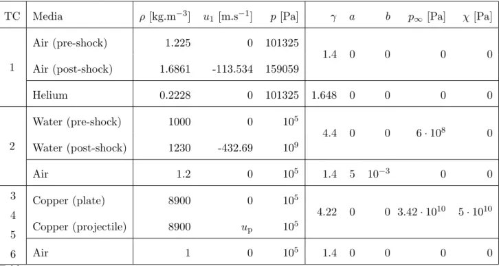
Table 1 shows the material properties and initial conditions relative to each test case.
TC Media ρ [kg.m−3] u1 [m.s−1] p[Pa] γ a b p∞ [Pa] χ[Pa]
1 Air (pre-shock) 1.225 0 101325 1.4 0 0 0 0 Air (post-shock) 1.6861 -113.534 159059 Helium 0.2228 0 101325 1.648 0 0 0 0 2 Water (pre-shock) 1000 0 105 4.4 0 0 6·108 0 Water (post-shock) 1230 -432.69 109 Air 1.2 0 105 1.4 5 10−3 0 0 3 4 5 6 Copper (plate) 8900 0 105 4.22 0 0 3.42·1010 5·1010 Copper (projectile) 8900 up 105 Air 1 0 105 1.4 0 0 0 0 Table 1
Test cases description.
6.1 Shock-bubble interaction
We consider two shock-bubble interaction test cases involving different fluids. The boundary conditions are fixed at the initial values for inlet and homo-geneous Neumann conditions are imposed at outlet. Reflection conditions are imposed for all the other boundaries.
Air-helium shock-bubble interaction
TC1 is the propagation in air of a Mach 1.22 shock through an helium bubble. The initial configuration and the physical parameters are described in Fig. 5
and in Table 1. The computation is performed on a 1000×400×400 mesh and lasts for 50h on 300 processors. The zero iso-value of the level set function and schlieren on the horizontal plane through the center of the bubble are presented at different times on Fig.6.
x y z 222.5mm 89mm 89mm 10mm 44.5mm 44.5mm 172.5mm 25mm Helium Air (pre-shock) Air (post-shock)
Fig. 5. Sketch of the initial configuration for the shock-bubble interaction TC1. The computational domain is [247.5,470]×[0,89]×[0,89]mm.
Fig. 6. Interaction of a Mach 1.22 shock propagating in air through an helium bubble (TC1). Pictures att= 62µs, 110µs, 163µs, 264µs, 471µs, 735µs. From left to right, top to bottom.
The results are qualitatively similar to those presented in the literature in two dimensions, see for example [28,12,22,16].
Air-water shock-bubble interaction
TC2 involves a van der Waals gas bubble and a Mach 1.422 shock in water modeled by a stiffened gas constitutive law. The initial configuration and the physical parameters are described in Fig. 7 and in Table 1. This test case is more severe compared to the previous one since it presents larger density ratios. The mesh is 480× 400× 400 and the computation lasts 15h on 96 processors. The results are presented in Fig.8, where we show the zero of the level set function and the schlieren on the vertical plane through the center of
the bubble. x y z 1.2m 1m 1m 0.25m 0.5m 0.5m 0.7m 0.2m Air Water (pre-shock) Water (post-shock)
Fig. 7. Sketch of the initial configuration for shock-bubble interaction TC2. The computational domain is [−0.2,1]×[0,1]×[0,1]m.
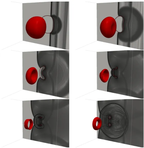
Fig. 8. Interaction of a Mach 1.422 water shock and an air bubble (TC2). Interface and schlieren on the plane z = 0.5 at time t = 37µs, 73µs, 110µs, 132µs, 147µs, 195µs. From left to right, top to bottom.
The bubble is strongly compressed, it changes topology and swirls similarly to what happens in two dimensions, see [1,16].
6.2 Impact
We present an impact simulation of a 800m.s−1 projectile on a plate in air (TC3). The initial configuration and the physical parameters are described in Fig. 9 and in Table 1. In this simulation the projectile and the plate are adjacent at initial time. The projectile and the plate are a single material and
they are described by the same level set. In other words they will necessarily stick together for the whole simulation. Homogeneous Neumann conditions are imposed at the borders. The computation is performed on a 6003 mesh and uses 216 processors for 60h.
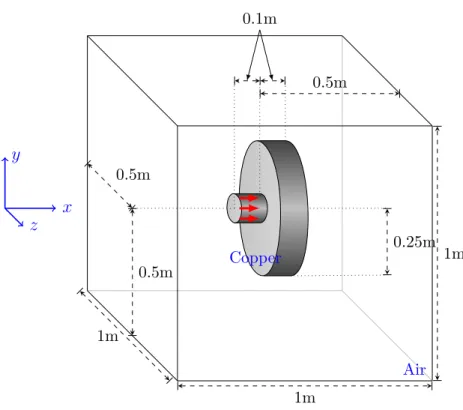
x y z 0.5m 0.5m 0.1m 1m 1m 1m 0.5m 0.25m Air Copper
Fig. 9. Sketch of the 3D initial configuration for the impact test case TC3 where a projectile impinges on a cylindrical plate with a velocity of 800m.s−1. The compu-tational domain is [−0.5,0.5]3m.
The results are shown on Fig. 10. The elastic material is deformed and oscil-lates while being displaced rightward. Schlieren images on the planesx= 0.03,
y = 0 and z = 0 are presented. Compared to the two dimensional test case [16] the deformation is less evident as the mass ratio between the projectile and the plate is smaller.
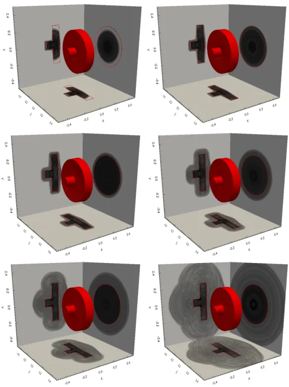
Fig. 10. Impact of a projectile on a plate (TC3). Interface and schlieren att= 24µs, 43µs, 88µs, 178µs, 355µs, 710µs. From left to right, top to bottom.
For this test case we present in Tab.2the convergence of the mass and energy conservation errors as functions of the grid refinement. The errors are com-puted by relative L1 norms in space and time. The simulations last until the
fluxes are zero across the domain boundaries for a mesh of 1003. This time represents 25% of the total computational time (fourth snapshot in Fig.10). It can be observed that the conservation errors coherently decrease as the mesh is refined with a rate close to 1, as expected. However, for large elongations of the material, like in the case of rubbers, conservation errors may occur due to the level set discretization. For long filaments, it may occur that when a structure is smaller than a computational cell, the isoline zero of the level set function disappears, and with it, the material contained.
L1 error 1003 2003 4003
Mass conservation (%) 0.6117 0.2602 0.1145
Energy conservation (%) 0.6155 0.2596 0.1137
Table 2
Mass and energy conservationL1errors in space and time in percentage of the total mass and energy, respectively, for mesh sizes of 1003, 2003 and 4003 (TC3).
Also, we show in Tab.3the relative error betweenρandρ0det(∇xY), and the
Frobenius norm of∇x× ∇xY for several mesh sizes. For these computations,
we only consider solid cells situated at a distance of 0.025m from the interface in order to avoid the singularity of the inverse deformation tensor at the border of the elastic solids. The simulations last about half the total computational time (fifth snapshot in Fig. 10). It can be seen that the errors decrease as the mesh is refined, at a rate that is of about 1 for the density, and slightly smaller for ∇x× ∇xY, as expected because of the additional differentiation.
L1 error 1003 2003 4003
|ρ−ρ0det(∇xY)|(%) 0.2300 0.1456 0.0511
k∇x× ∇xYk 0.1716 0.1258 0.0768
Table 3
L1-norm error in space and time of |ρ−ρ0det(∇xY)| in percentage of ρ and L1
-Frobenius norm in space and time of ∇x×(∇xY) for mesh sizes of 1003, 2003 and
6.3 Rebounds
We now focus on cases similar to impacts except that the projectile is not initially adjacent to the plate and can rebound. Here we do not consider the modeling of the full relevant physics at the scales induced by the arbitrarily small gap between the objects getting in contact. However, in terms of numer-ical modeling this case may need special care in the solution of the Riemann problem when the projectile and the plate get in material contact. Material contact is defined as a configuration where the level sets pertaining to the projectile and the plate are separated by less than a grid point. We model this phenomenon as a frictionless contact where both the normal and the tangen-tial stresses vanish. This allows a discontinuity in both normal and tangentangen-tial velocities in the solution of the Riemann problem, see equations (53),(54) and (55).
Two-dimensional rebounds
First, we simulate the solution in two dimensions as the meshes that can be afforded are significantly finer. As depicted on Fig. 11, the first test case is relative to a copper disk moving toward a copper layer on the east boundary. The surrounding fluid is air. The east border of the computational domain acts as a rigid wall where the displacement vanishes in the normal direction. The other borders are modeled by homogeneous Neumann conditions.
The gap between the disk and the plate measures 10−2m and the disk travels at a speed of 500m.s−1. A few snapshots of the solution are presented on Fig12. The computations are run on 20002 and 40002 meshes. The computations last 10h and 12h on 144 and 324 processors, respectively.
2m 2m 1m 0.5m ∅1m 0.01m Copper Air Copper
Fig. 11. Sketch of the 2D initial configuration for impact and rebound test case TC4 where a copper disk impinges on a copper layer at velocity 500m.s−1. The computational domain is [−1,1]2m.
150 300 450 0.000e+00 5.018e+02 Velocity (m/s) 1.0 -0.5 -1.0 0.0 0.5 0.0 0.5 -1.0 -0.5 1.0 1.0 -0.5 -1.0 0.0 0.5 0.0 0.5 -1.0 -0.5 1.0 150 300 450 0.000e+00 5.012e+02 Velocity (m/s) 2500 5000 7500 0.000e+00 1.052e+04 Velocity (m/s) 1.0 -0.5 -1.0 0.0 0.5 0.0 0.5 -1.0 -0.5 1.0 1.0 -0.5 -1.0 0.0 0.5 0.0 0.5 -1.0 -0.5 1.0 2000 4000 6000 8000 0.000e+00 9.688e+03 Velocity (m/s) 1500 3000 4500 0.000e+00 5.729e+03 Velocity (m/s) 1.0 -0.5 -1.0 0.0 0.5 0.0 0.5 -1.0 -0.5 1.0 1.0 -0.5 -1.0 0.0 0.5 0.0 0.5 -1.0 -0.5 1.0 1500 3000 4500 0.000e+00 5.974e+03 Velocity (m/s)
Fig. 12. Impact and rebound of a projectile on a layer in two dimensions. Velocity and schlieren at timet= 21µs, t= 450µs and t= 900µs from top to bottom. The mesh is 20002 on the left and 40002 on the right.
In the case where the mesh is 20002, the rebound takes place thanks to a material contact of the disk with the copper layer. An high speed shock and the corresponding jet emerge from the impact. When the mesh size increases to 40002 cells, no contact occurs at the rebound and a thin layer of air cells
still separates the two materials. The flow and deformation features observed for a 20002 mesh are overall retrieved for a 40002 mesh.
The pressure through y= 0 for both meshes is presented on Fig. 13. We can observe a significant pressure peak at the contact interface compressing the material and therefore the surrounding fluid that is ejected from the contact region at high speed.
−0.4 −0.2 0 0.2 0.4 0.6 0.8 1 10 20 30 40 50 60 70 80 90 x (m) p+p ∞ (GPa) Mesh 20002 Mesh 40002
Fig. 13. Pressure on the line y= 0 in the range x∈[−0.4,1] at timet= 450µs.
TC5 is relative to the impact of a the projectile at 800m.s−1 initially detached from a shield in two dimensions. The initial configuration and the physical parameters of the two-dimensional simulation are described in Fig. 14 and in Table 1. The computation is performed on a 40002 mesh and uses 242 processors for 6 hours.
1m 1m 0.5m 0.1m 0.5m 0.05m 0.5m ∅0.1m Copper Air
Fig. 14. Sketch of the 2D initial configuration for impact and rebound test case TC5 where a projectile impinges a plate at velocity 800m.s−1. The computational domain is [−0.5,0.5]2m.
Here the disk actually rebounds on an shock layer created in front of the disk. This layer has a thickness of a few grid points. Again a high speed shock forms at the impact. The speed of this shock is of the order of that of the fast waves in the elastic solid. These results show that the overall scheme is robust on very fine meshes for stiff numerical simulations.
Three-dimensional rebound
The initial configuration and the physical parameters of the three-dimensional rebound (TC6) are described in Fig. 16 and in Table 1. The computation is performed on a 4003 mesh and uses 216 processors for 24 hours.
x y z 0.5m 0.5m 0.1m 1m 1m 1m 0.5m 0.3m ∅ 0.2m
Fig. 16. Sketch of the initial configuration for the impact test case TC6 where a projectile impinges a shield at velocity 800m.s−1 and rebounds. The computational domain is [−0.5,0.5]3m.
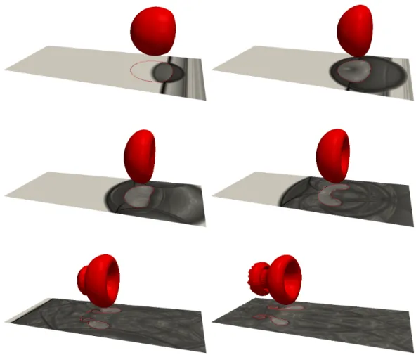
Fig. 17. Impact of a projectile on a shield (TC6). Interface and schlieren on the planes x = 0.025 and y =z = 0 at t = 107µs, 166µs, 206µs, 256µs, 383µs, 710µs. From left to right, top to bottom.
Overall the physics of the interaction is similar to what observed in two di-mensions. In the figure the level set of the shield is in blue, whereas as the sphere is red. The level sets are also projected on the visualized planes.
7 Conclusions and Future Work
We have presented a three-dimensional multimaterial model that describes the dynamics of the interaction between gas, liquids and neohookean materials. This model is hyperbolic and reduces to the well known linear model in the small-deformation limit. The numerical scheme is based on an approximate Riemann solver that is able to model multimaterial interfaces with possibly frictionless contacts. The scheme is simple to implement, stable and robust, as shown by the stiff test cases presented.
The explicit solver proposed is constrained by the time scale of the elastic waves. For problems such as impacts or in general fast-dynamical processes, this is the relevant scale of the physical phenomenon. For physical phenom-ena that take place on the time scale determined by the material velocity, the stability condition limits the application of such time-dependent approaches. Also, the significantly different time scales present in multimaterial phenomena introduce accuracy and efficiency problems that are well known in low-speed compressible fluids. Future work will include exploration of these issues for compressible multimaterial flows, as well as, enriching the model with plastic-ity.
Acknowledgements
This study has been carried out with financial support from the French State, managed by the French National Research Agency (ANR) in the frame of the Investments for the future Programme IdEx Bordeaux-CPU (ANR-10-IDEX-03- 02). The simulations presented in this paper were carried out using the PLAFRIM experimental parallel testbed, being developed under the Inria PlaFRIM development action with support from LABRI and IMB and other entities: Conseil R´egional d’Aquitaine, FeDER, Universit´e de Bordeaux and
CNRS (see https://plafrim.bordeaux.inria.fr/). Alexia De Brauer is supported by a grant from the DGA (D´el´egation G´en´erale de l’Armement, Minist`ere de la D´efense).
References
[1] G. Allaire, S. Clerc, and S. Kokh. A five-equation model for the simulation of interfaces between compressible fluids. Journal of Computational Physics, 181(2):577–616, 2002. 30
[2] P.T. Barton, R. Deiterding, D. Meiron, and D. Pullin. Eulerian adaptive finite-difference method for high-velocity impact and penetration problems. Journal of Computational Physics, 240(C):76–99, 2013. 3
[3] P.T. Barton and D. Drikakis. An Eulerian method for multi-component
problems in non-linear elasticity with sliding interfaces. Journal of Computational Physics, 229(15):5518–5540, 2010. 3
[4] P.T. Barton, D. Drikakis, E. Romenski, and V.A. Titarev. Exact and
approximate solutions of Riemann problems in non-linear elasticity. Journal of Computational Physics, 228(18):7046–7068, 2009. 3
[5] P.T. Barton, B. Obadia, and D. Drikakis. A conservative level-set based method for compressible solid/fluid problems on fixed grids . Journal of Computational Physics, 230(21):7867–7890, 2011. 3
[6] M. Berndt, J. Breil, S. Galera, M. Kucharik, P.-H. Maire, and
M. Shashkov. Two-step hybrid conservative remapping for multimaterial arbitrary Lagrangian-Eulerian methods. Journal of Computational Physics, 230(17):6664–6687, 2011. 2
[7] G.H. Cottet, E. Maitre, and T. Milcent. Eulerian formulation and level set models for incompressible fluid-structure interaction. ESAIM: Mathematical Modelling and Numerical Analysis, 42:471–492, 2008. 4,5
[8] S. Davis. Simplified second-order Godunov-type methods. SIAM Journal on Scientific and Statistical Computing, 9(3):445–473, 1988. 22
[9] N. Favrie, S Gavrilyuk, and S Ndanou. A thermodynamically compatible
splitting procedure in hyperelasticity. Journal of Computational Physics, 270(C):300–324, 2014. 3
[10] N. Favrie and S. L. Gavrilyuk. Diffuse interface model for compressible fluid – Compressible elastic-plastic solid interaction. Journal of Computational Physics, 231(7):2695–2723, 2012. 3
[11] N. Favrie, S.L. Gavrilyuk, and R. Saurel. Solid-fluid diffuse interface model in cases of extreme deformations. Journal of Computational Physics, 228(16):6037–6077, 2009. 2,3,4,8
[12] R.P. Fedkiw, T. Aslam, B. Merriman, and S. Osher. A non-oscillatory Eulerian approach to interfaces in multimaterial flows (the ghost fluid method). Journal of Computational Physics, 152:457–492, 1999. 2,28
[13] S. Galera, P.-H. Maire, and J. Breil. A two-dimensional unstructured cell-centered multi-material ALE scheme using VOF interface reconstruction. Journal of Computational Physics, 229(16):5755–5787, 2010. 2
[14] S.L. Gavrilyuk, N. Favrie, and R. Saurel. Modelling wave dynamics of compressible elastic materials. Journal of Computational Physics, 227(5):2941– 2969, 2008. 3,8,18
[15] S.K. Godunov. Elements of continuum mechanics. Nauka Moscow, 1978. 2,4
[16] Y. Gorsse, A. Iollo, T. Milcent, and H. Telib. A simple cartesian scheme for compressible multimaterials. Journal of Computational Physics, 272:772–798, 2014. 3,4,11,18,22,23,24,28,30,31
[17] D.J. Hill, D. Pullin, M. Ortiz, and D. Meiron. An Eulerian hybrid WENO centered-difference solver for elasticplastic solids. Journal of Computational Physics, 229(24):9053–9072, 2010. 3
[18] G.A. Holzapfel. Nonlinear Solid Mechanics. A continuum approach for
engineering. J. Wiley and Sons, 2000. 6,7
[19] G.S. Jiang and C.W. Shu. Efficient implementation of Weighted ENO schemes. Journal of Computational Physics, 126(1):202–228, 1996. 25
[20] G. Kluth and B. Despres. Discretization of hyperelasticity on unstructured mesh with a cell-centered Lagrangian scheme. Journal of Computational Physics, 229(24):9092–9118, 2010. 2
[21] P.-H. Maire, R. Abgrall, J. Breil, R. Loub`ere, and B. Rebourcet. A nominally second-order cell-centered Lagrangian scheme for simulating elastic-plastic flows on two-dimensional unstructured grids. Journal of Computational Physics, 235(C):626–665, 2013. 2
[22] A. Marquina and P. Mulet. A flux-split algorithm applied to conservative models for multicomponent compressible flows. Journal of Computational Physics, 185(1):120–138, 2003. 28
[23] G.H. Miller. An iterative Riemann solver for systems of hyperbolic
conservation laws, with application to hyperelastic solid mechanics. Journal of Computational Physics, 193(1):198–225, 2003. 3
[24] G.H. Miller and P. Colella. A conservative three-dimensional eulerian method for coupled solid-fluid shock capturing. Journal of Computational Physics, 183(1):26–82, 2002. 2,4
[25] S Ndanou, N. Favrie, and S Gavrilyuk. Criterion of hyperbolicity in
hyperelasticity in the case of the stored energy in separable form. Journal of Elasticity, 115(1):1–25, 2013. 13
[26] B.J. Plohr and D.H. Sharp. A conservative eulerian formulation of the equations for elastic flow. Advances in Applied Mathematics, 9:481–499, 1988. 2,4
[27] B.J. Plohr and D.H. Sharp. A conservative formulation for plasticity. Advances in Applied Mathematics, 13:462–493, 1992. 2,4
[28] J. Quirk and S. Karni. On the dynamics of a shock-bubble interaction. Journal of Fluid Mechanics, 318(1):129–163, 1996. 28
[29] E.F. Toro, M. Spruce, and W. Speares. Restoration of the contact surface in the HLL-Riemann solver. Shock Waves, 4:25–34, 1994. 18


![Fig. 5. Sketch of the initial configuration for the shock-bubble interaction TC1. The computational domain is [247.5, 470] × [0, 89] × [0, 89]mm.](https://thumb-us.123doks.com/thumbv2/123dok_us/9665223.2454494/28.892.137.777.751.999/sketch-initial-configuration-shock-bubble-interaction-computational-domain.webp)
![Fig. 7. Sketch of the initial configuration for shock-bubble interaction TC2. The computational domain is [−0.2, 1] × [0, 1] × [0, 1]m.](https://thumb-us.123doks.com/thumbv2/123dok_us/9665223.2454494/30.892.195.692.653.1018/sketch-initial-configuration-shock-bubble-interaction-computational-domain.webp)