In Proc. AAMAS Workshop on Agent Mediated Electronic Commerce VI, July 2004.
Three Automated Stock-Trading Agents:
A Comparative Study
Alexander A. Sherstov and Peter Stone The University of Texas at Austin Department of Computer Sciences
Austin, TX 78712 USA
{sherstov, pstone}@cs.utexas.edu
Abstract. This paper documents the development of three autonomous
stock-trading agents within the framework of the Penn Exchange Simulator (PXS), a novel stock-trading simulator that takes advantage of electronic crossing net-works to realistically mix agent bids with bids from the real stock market [1]. The three approaches presented take inspiration from reinforcement learning, myopic trading using regression-based price prediction, and market making. These ap-proaches are fully implemented and tested with results reported here, including individual evaluations using a fixed opponent strategy and a comparative analysis of the strategies in a joint simulation. The market-making strategy described in this paper was the winner in the fall 2003 PLAT live competition and the runner-up in the spring 2004 live competition, exhibiting consistent profitability. The strategy’s performance in the live competitions is presented and analyzed.
1
Introduction
Automated stock trading is a burgeoning research area with important practical applica-tions. The advent of the Internet has radically transformed the nature of stock trading in most stock exchanges. Traders can now readily purchase and sell stock from a remote site using Internet-based order submission protocols. Additionally, traders can moni-tor the contents of buy and sell order books in real time using a Web-based interface. The electronic nature of the transactions and the availability of up-to-date order-book data make autonomous stock-trading applications a promising alternative to immediate human involvement.
The work reported here was conducted in the Penn Exchange Simulator (PXS), a novel stock-trading simulator that takes advantage of electronic crossing networks to realistically mix agent bids with bids from the real stock market [1]. In preparation for an open live competition, we developed three parameterizable trading agents and defined several instantiations of each strategy. We optimized each agent independently, and then conducted detailed controlled experiments to select the strongest of the three for entry in the live competition.
It is important to realize from the outset that this research is primarily an agent
study pertaining to the interactions of particular agents in a fixed economy. Although
PXS makes a strong and reasonable claim to implementing a realistic simulation of the stock market, the results and conclusions in this paper pertain to test economies includ-ing specific other stock-tradinclud-ing agents. In particular, we do not aim to create strategies
that are ready for profitable deployment in the real stock market (otherwise we would likely not be writing this paper!). Rather, this paper makes three main contributions. First, it contributes an empirical methodology for studying and comparing stock-trading agents—individually as well as jointly in a shared economy—in a controlled empiri-cal setting. Second, it implements this methodology to compare three specific trading agents based on reinforcement learning, myopic trading using regression-based price prediction, and market making. Third, this paper contributes detailed specifications of promising strategy designs, one of which vastly outperformed competitor strategies in an open stock-trading competition and exhibited consistent profitability under a variety of market conditions.
The remainder of the paper is organized as follows. Section 2 provides the relevant technical background on the PXS simulator, our substrate domain. Section 3 charac-terizes prior research and points out the distinguishing features of this work. Section 4 discusses our approach to the automated stock-trading problem, explains our assump-tions, and details our experimental methodology. Sections 5–7 describe our three stock-trading strategies. Sections 8–10 present and analyze the experimental results, focusing, respectively, on individual evaluations, the joint simulation, and the live competitions. Finally, Section 11 concludes with a discussion of unresolved questions and promising directions for future work.
2
Background
The Penn-Lehman Automated Trading (PLAT) project [1] is a research initiative de-signed to provide a realistic testbed for stock-trading strategies. PLAT provides a sim-ulated stock-trading environment known as the Penn Exchange Simulator (PXS) that merges virtual orders submitted by computer programs with real-time orders from the Island electronic crossing network (ECN) [2]. No actual monetary transactions are con-ducted, and the efficacy of a trading strategy can be reliably assessed in the safety of a simulated market. Many previous stock simulators been developed that execute simu-lated orders at the current price in the real stock market. However, such simulators miss the effect of a simulated order on this price, an effect that becomes increasingly signifi-cant as the size of the orders increases. The main novelty of PXS is that it uses not only the current stock price, but also the whole list of pending limit orders to realistically determine the effect of simulated activity on the market [1].
PXS operates in cycles. During every cycle, a trading agent can place new orders and/or withdraw some of its previously placed orders. When placing a buy order, the agent specifies the number of shares it wishes to purchase and the highest price per share it is willing to pay. PXS sorts the buy orders by price into a buy order book, with the most competitive (highest-priced) orders at the top of the book. Likewise, a sell
order states the amount of stock being sold and the lowest price per share the seller
is willing to accept. PXS sorts the sell orders into a sell order book, with the most competitive (lowest-priced) orders on top. When an order arrives, PXS matches it with orders in the opposite order book (starting at the top of the book) that meet the order’s price requirements. Partial matches are supported. Any unmatched portion of the order is placed in the corresponding book, awaiting competitive enough counterpart orders to match fully.
Apart from complete order-book data, the simulator makes a variety of agent-specific and market-wide information available to aid in order placement. In addition to real-time operation (live mode), the simulator supports historical simulations that use archived stock-market data from the requested day. Historical mode operates on a compressed time scale, allowing the simulation of an entire trading day in minutes. As a result, the agent is able to place considerably fewer orders overall than in live mode. Aside from the lower order-placement frequency, historical mode is operationally iden-tical to live mode.
In December 2003 and April 2004, live PLAT stock-trading competitions were held including agents from several universities. The sole performance criterion was the Sharpe ratio, defined as the average of the trader’s daily score over several days di-vided by the standard deviation. Thus, favorable placement in the competition required not only sizable daily earnings but also consistent day-to-day performance. The trader’s score on a given trading day was its total profit and loss (“value”) at the end of the day
plus total “rebate value” (computed as $0.002 per share that added liquidity to the
simu-lator) minus total “fee value” (computed as $0.003 per share that removed liquidity from the simulator). These rebates and fees are the same as those used by the Island ECN. Arbitrarily large positive or negative intra-day share holdings were allowed. However, the entrants were to completely unwind their share positions before the end of the day (i.e., sell any owned shares and buy back any owed shares) or face severe monetary penalties.
As a benchmark strategy for the experiments reported in this paper, we used the Static Order-Book Imbalance (SOBI) strategy [1], provided to participants in the PLAT competition as an example trading agent. We used default settings for all SOBI pa-rameters. SOBI sells stock when the volume-weighted average price (VWAP) of the buy-book orders is further from the last price than the sell-book VWAP, interpreting this as weaker support for the current price on the buyers’ part and a likely depreciation of the stock in the near future. In the symmetric scenario, SOBI places buy orders.
3
Related Work
Prior research features a variety of approaches to stock trading, including those pre-sented here. Automated market making has been studied in [3–5]. Reinforcement learn-ing has been previously used to adjust the parameters of a market-maklearn-ing strategy in response to market behavior [3]. Other approaches to automated stock trading include the reverse strategy and VWAP trading [5, 6]. A brief overview of these common ap-proaches can be found in [7].
To our knowledge, there have been no empirical studies of the interactions of het-erogeneous strategies in a joint economy, yet such simulations would likely be more revealing of a strategy’s earning potential than a study of the strategy in isolation. As a result, this work combines detailed individual evaluations of the strategies with a prin-cipled study of their performance in a joint economy. Another distinguishing feature of this research is the use of a highly realistic stock simulator. Furthermore, this research bases performance evaluations on the Sharpe ratio, a reliable measure of “the statistical significance of earnings and the trade-off between risk and return” [1]. The Sharpe ratio is “the most widely-used measure of risk-adjusted return,” a quantity most modern fund
managers seek to maximize (rather than raw profits) [8]. Unfortunately, the Sharpe ratio has seen little use in the automated stock-trading literature.
The strategies themselves certainly do set this work apart from previous research. Specifically, we know of no other research applying reinforcement learning to the com-plete stock-trading task. Moreover, the exact design and parameterization of the trend-following and market-making strategies used in this paper have likely not been tried elsewhere. However, what truly makes this work original are the principled compar-isons of the strategies in a novel, more realistic setting, with a relatively uncommon and valuable performance metric.
4
Approach and Assumptions
The generic stock-trading agent architecture used throughout this paper is illustrated in Figure 1. The PLAT competition does not allow share/cash carryover from one trading day to the next. This algorithm is therefore designed to run from 9:30 a.m. to 4 p.m., the normal trading hours, maximizing profits on a single day (lines 1–4) and completely un-winding the share position before market close (lines 5–9). The actual trading strategy is abstracted into the COMPUTE-ACTIONroutine. Given the system’s state, this routine prescribes the withdrawal of some of the previously submitted orders and/or the place-ment of new orders, each given by a type (BUYorSELL), volume, and price. Sections 5, 6, and 7 explore distinct implementations of this routine.
GENERIC-TRADING-AGENT
1 whilecurrent-time<3 p.m.
2 dostate←updated trader, market stats; action←COMPUTE-ACTION(state) 3 ifaction6=VOID
4 then place/withdraw orders peraction 5 withdraw all unmatched orders
6 while market open ¤unwind share position
7 dostate←updated trader, market stats 8 ifshare-position6= 0
9 then match up to|share-position|shares of top order in opposite book
Fig. 1. Generic agent architecture
Position unwinding (lines 5–9 in Figure 1) works as follows. The agent starts by withdrawing all its unmatched orders. Then, if the agent owes shares (has sold more than it has purchased), it places a buy order, one per order placement cycle, forsshares at pricep, wheresandpare the volume and price of the top order in the sell book. The liquidation of any owned shares proceeds likewise. This unwinding method allows for rapid unwinding at a tolerable cost. By spacing the unwinding over multiple cycles, this scheme avoids eating too far into the books. By contrast, a scheme that simply places a single liquidating order is unable to take advantage of future liquidity and possibly better prices.
The fundamental assumption underlying the generic agent design of Figure 1 is that profit maximization and position unwinding are two distinct objectives that the automated trading application can treat separately. Although this task decomposition may be suboptimal, it greatly simplifies automated trader design. Moreover, the profit-maximization strategies proposed in this paper, perhaps with the exception of the
ap-proach based on reinforcement learning, hold very reasonable share positions through-out the day, making unwinding feasible at a nominal cost. The time of the phase shift between profit maximization and position unwinding (3 p.m.) was heuristically chosen so as to leave more than enough time for fully unwinding the agent’s position.
We have adopted the following experimental methodology in this paper. First, we developed three parameterizable strategies (implementations of the COMPUTE
-ACTIONroutine) and defined several instantiations of each strategy. Next, we evaluated
each instantiation separately, in a controlled setting, using SOBI as a fixed opponent strategy. In what follows, we describe only the most successful instantiation of each strategy. Finally, we identified the most successful strategy among these by means of a joint simulation. The live competitions, albeit not controlled experiments, have offered additional empirical feedback.
5
The Reinforcement Learning Agent
Reinforcement learning [9] is a machine-learning methodology for achieving good long-term performance in poorly understood and possibly non-stationary environments. Given the seemingly random nature of market fluctuations, it is tempting to resort to a model-free technique designed to optimize performance given minimal domain exper-tise and a reasonable measure of progress. A machine-learning approach to this problem is further motivated by the need to adapt to the economy (particular mix of opponents, market performance, etc.). A fixed, hand-coded strategy can hardly account for all con-tingencies.
In its simplest form, a reinforcement learning problem is given by a 4-tuple {S,A, T, R}, whereS is a finite set of the environment’s states;Ais a finite set of actions available to the agent as a means of extracting an economic benefit from the environment, referred to as reward, and possibly of altering the environment state;
T :S × A → S is a state transition function; andR :S × A → Ris a reward func-tion. The state transition and reward functions T andR are possibly stochastic and unknown to the agent. The objective is to develop a policy, i.e., a mapping from envi-ronment states to actions, that maximizes the long-term return. A common definition of return, and one used in this work, is the discounted sum of rewards:P∞t=0γtrt, where
0< γ <1is a discount factor andrtis the reward received at timet.
The original RL framework was designed for discrete state-action spaces. In order to accommodate the continuous nature of the problem, we used tile coding, a linear function-approximation method, to allow for generalization to unseen instances of the continuous state-action space.
5.1 Strategy Design
Since the transition functionT is an unknown feature of the environment meant to be learned by the agent, the design of a trading strategy reduces to the specification of the state-action space and the reward function. After exploring several formulations of the stock-trading problem as a reinforcement-learning task, we adopted the following design:
State space. The state space is given by a single variable, the price parameter∆pt=
pt−pt, computed as the difference between the current last price and an exponential average of previous last prices:pt = βpt−1+ (1−β)pt. The effect ofβ is to focus
the agent on short-term or long-term trends (see Section 5.2 for an experimental study of this effect). The definition of the price parameter as a difference serves a twofold purpose. On the one hand, it gives an indication of the latest market trend:∆p ≈ 0 corresponds to a stationary market, ∆p < 0 corresponds to a decline in price, and
∆p > 0indicates that the stock price is on the rise. On the other hand, this definition makes the learned policy more general by eliminating the dependency on the absolute values of the prices.
We limited the state space to the price parameter for the following reasons. First of all, share and cash holdings are of no use as state variables: the “right” trading decision is never contingent on these parameters because the agents are allowed to have an arbi-trarily large positive or negative share/cash position, and position unwinding is no part of the profit-maximization strategy. For the same reason, a “remaining time” parameter would not be helpful either. Although additional state variables might have been useful, we decided to avoid the corresponding increase in complexity.
Action space. The action space is likewise given by a single variable, the volume of
shares to purchase or sell. We limited the range of this variable to[−900,900], with negative values corresponding to sell orders and positive values, to buy orders. This trade size is a very generous leash, allowing rapid accumulation of share positions as large as 150,000 shares and beyond. To save a dimension of complexity, we decided against extending the action space to include order price. Instead, we always set the price of an order to the last price, leaving it up to the agent to adjust the demanded volume accordingly.
Reward function. Ideally, the reward should be computed only once, at the end of
the trading day, with zero intermediate rewards assigned at each time step along the way; otherwise, there is a danger that the trader will learn to optimize the sum of local rewards without optimizing the final position ([9], Chapter 3). There are two important complications with this approach. First, it rules out on-line adjustment to the economy. Second, given the complexity of the state-action space (2 continuous variables) and the duration of a simulation (≈50,000 order placement cycles in live mode), the training time requirements of this method seem excessive. Instead, we use a localized reward function, given by the difference in present value (cash holdings plus shares valued at the last price) from the last time step.
5.2 Parameter Choices
We used the Sarsa algorithm [10, 11] with the following parameters:α= 0.04,γ= 0.8,
² = 0.1, andλ = 0.7. We have not experimented with varying these values and used them as reasonable general settings. A final parameter that played a substan-tial role wasβ, the update rate for computing the exponential average of past prices:
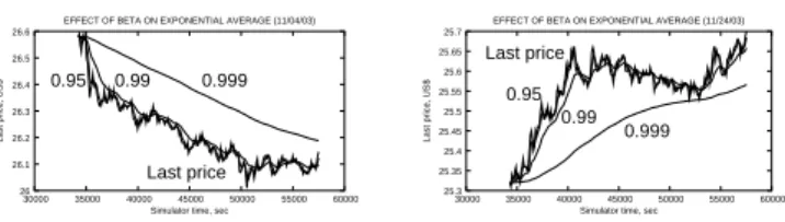
pt =βpt−1+ (1−β)pt. Figure 2 demonstrates the behavior of the average price on two trading days with different price dynamics andβ settings. As the graphs indicate, the closerβ is to 1, the more “inert” the exponential average, i.e., the less responsive to changes in the price trend. On the one extreme,β = 0.95essentially duplicates the last price graph, yielding little information about past price dynamics. On the other ex-treme,β = 0.999 yields an average that is not at all representative of the changes in price dynamics. The graphs indicate that a choice ofβ = 0.99offers a nice balance,
responding sufficiently quickly to genuine trend reversals and ignoring random fluctu-ations. We use this informed heuristic choice forβin our experiments, leaving a more detailed optimization with respect to actual performance for future work.
Last price 0.999 0.95 0.99 26 26.1 26.2 26.3 26.4 26.5 26.6 30000 35000 40000 45000 50000 55000 60000
Last price, US$
Simulator time, sec EFFECT OF BETA ON EXPONENTIAL AVERAGE (11/04/03)
25.3 25.35 25.4 25.45 25.5 25.55 25.6 25.65 25.7 30000 35000 40000 45000 50000 55000 60000
Last price, US$
Simulator time, sec EFFECT OF BETA ON EXPONENTIAL AVERAGE (11/24/03)
0.999 0.95
Last price
0.99
Fig. 2. Effect ofβon price average
The strategy was trained on 250 historical simulations, each encompassing over 15,000 order placement cycles, for a total of nearly 4 million Bellman backups. This amount of training effort was deemed to provide the agent with sufficient experience. Each simulation involved SOBI as the agent’s only opponent. The trading days were a random mix of trading days in October 2003, similar in composition to the handpicked collection of days on which performance was measured. The agent functioned in learn-ing mode (i.e., uslearn-ing the original settlearn-ings of the learnlearn-ing and exploration rates) durlearn-ing evaluative simulations to allow on-line adjustment to the economy.
6
The Trend-following Agent
Our second agent uses a trend-following (TF) approach based on price prediction. Un-like reinforcement learning, this approach constructs an explicit model of market dy-namics, based on linear regression, to guide order placement. Roughly, the strategy is as follows. If the price is rising (i.e., the slope of the regression line is positive), the agent places buy orders, confident that it will be able to sell the purchased shares back at a higher price. If, on the other hand, the price is falling, the agent will place sell orders. In either case, the agent attempts to unwind its share position just before the price starts to drop (if it is currently on the rise) or just before the price starts to rise (if it is currently on the decline).
The details of the TF approach are best illustrated through an example. Figures 3a and 3b show, respectively, the Island last price on November 18, 2003, and the first and second derivatives1P0andP00of the price function (scaled differently to permit display on the same set of axes). The value of theP0 curve at timetis the slope of the linear regression line computed using the price data for the past hour, i.e., for the time interval
[t−3600, t], wheretis expressed in seconds. The length of the time interval presents a trade-off between currency (shorter time intervals generateP0 curves that are more responsive to price fluctuations) and stability (longer time intervals generateP0curves that are more “inert” and thus less susceptible to random fluctuations). We used an interval width of 1 hour, the duration of a typical medium-term trend, to balance these desirable characteristics. The purpose of theP0curve is to distill growth and decrease information from the price graph, detecting genuine long-term price trends and ignoring short-term random price fluctuations.
1As explained below,P0andP00extract growth information from series of price data, to account for its noisy nature. Therefore,P0andP00are not derivatives in the strict sense of the term since they do not capture instantaneous change, and we abuse this mathematical concept slightly here.
The value of theP00curve at timetis the slope of the linear regression line computed using theP0curve data for the past 400 seconds, i.e., over the time interval[t−400, t]. The width of the time interval over which the regression line is computed offers the same trade-off between responsiveness and stability; our experiments suggest that the value of 400 seconds offers a good balance. TheP00curve is above thex-axis whenever theP0 curve is exhibits growth, and below thex-axis whenever theP0curve is on the decline. Therefore, theP00(t)value changes sign whenever theP0curve reaches a local extremum, signaling a likely trend reversal in the near future. The purpose of theP00(t) is to alert the agent when the price trend is reversed.
price 25.1 25.2 25.3 25.4 25.5 25.6 25.7 25.8 25.9 30000 35000 40000 45000 50000 55000 60000 MSFT price, US$
Simulator time (sec) ISLAND LAST PRICE ON 11/18/03
P’ P’’ −15 −10 −5 0 5 10 15 20 35000 40000 45000 50000 55000 60000 Simulator time (sec)
P’ AND P’’ CURVES ON 11/18/03
a b
Fig. 3. Island last price on 11/18/2003 (a) and the correspondingP0
andP00
curves (b)
Figure 4 presents the trend-following strategy in pseudo-code. We used a trade size of 75 shares, a rather generous limit leading to share positions as large as 150,000 shares. Further increasing the trade size may complicate unwinding. Another essential component of the strategy is the order pricing scheme (lines 1–2). In the pseudo-code, we definedpredicted-last-price =a·tcurr+b, wheretcurris current time anda= P0(t
curr)andbare the parameters of the linear regression line fitted to the price data for the past hour. Our original implementation always stepped a fractional amount in front of the current top order, ensuring rapid matching of placed orders. The current strategy design uses a more cautious pricing scheme that experiments show results in systematically better performance.
COMPUTE-ACTION(state)
1 sell-price←max{last-price,predicted-last-price}
2 buy-price←min{last-price,predicted-last-price}
3 ifP0>0andP00>0
4 then return “BUY75 shares atbuy-price” 5 elseifP0<0andP00<0
6 then return “SELL75 shares atsell-price”
7 elseifshare-position6= 0 ¤reversal, so unwind 8 then withdraw unmatched orders
9 return “match up to|share-position|shares of top order in opposite book” 10 else return “VOID”
Fig. 4. The trend-following strategy
7
The Market-making Agent
As discussed above, the objective of the trend-following strategy is to look for long-term trends in price fluctuations, buying stock when the price is low and later selling stock when the price has gone up (and vice versa with the price going in the opposite
direction). As a result, the performance of the strategy is highly dependent on the price dynamics of a particular trading day. If more consistency is desired, an approach based on market making (MM) may be more useful. Unlike the trend-following strategy, the MM strategy capitalizes on small fluctuations rather than long-term trends and is likely to produce a smaller variance in profit.
Our final approach to the stock-trading problem combines the regression-based price prediction model presented in Section 6 with elements of market making. The strategy (Figure 5) still buys stock when the price is increasing at an increasing rate and sells stock when the price is decreasing at an increasing rate. However, rather than wait for a trend reversal to unwind the accumulated share position, the agent places buy and sell orders in pairs. When the price is increasing at an increasing rate, the agent places a buy order. As soon as this primary order is matched, the agent places a sell order at price
p+PM (the conditional order, so called because its placement is conditional on the matching of the primary order), confident that the latter will be matched shortly when the price has gone up enough. ThePM (profit margin) parameter is the per-share profit the agent expects to make on this transaction. Our implementation usesP M = $0.01 as a sufficiently profitable yet safe choice. The situation is symmetric when the price is decreasing at an increasing rate. Finally, the agent takes no action during periods des-ignated as “price reversal” by the prediction module (with price increasing/decreasing at a decreasing rate): since the orders are placed in pairs at what is deemed a “safe” time, no additional effort is called for to unwind the share position. The pricing scheme (stepping just behind the top order) is designed to avoid fees for removing liquidity, as discussed in Section 2.
COMPUTE-ACTION(state)
1 S←price of top sell order + $0.001 ¤sell price 2 B←price of top buy order - $0.001 ¤buy price 3 place qualifying conditional orders
4 ifP0>0andP00>0 5 then create conditional order
“SELL75 @B+PM” 6 return “BUY75 shares atB” 7 elseifP0<0andP00<0 8 then create conditional order
“BUY75 @S−PM” 9 return “SELL75 shares atS” 10 else return “VOID”
Fig. 5. The market-making strategy
M
M
F
F
Z
Z
Z
O
O
O
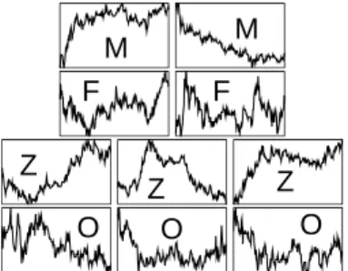
Fig. 6. Price dynamics (stock price vs. time)
on the 10 days used for strategy evaluation. Dates (left to right and top to bottom): 11/3, 4, 6, 19, 12, 18, 24, 21, 13, 26. (All dates in Oct. 2003.) Label legend: M=“monotonic,” F=“substantial fluctuation,” Z=“zigzag behav-ior,” O=“mixed (other).”
8
Individual Assessment
Our controlled experiments in this section and Section 9 use a set of 10 trading days carefully selected to represent typical price dynamics (Figure 6), namely, monotonic decrease/increase, substantial fluctuation, and zigzag and mixed behaviors. The graphs in Figure 6 are scaled differently and convey only the shape of the price curves. Each graph is labeled by a symbol denoting the price behavior, with a legend given in the
caption. Table 1 displays the raw profit/loss of the RL, TF, and MM strategies in in-dividual simulations against SOBI, with days labeled by price behavior (the labels are taken from Figure 6). The bottom row gives each strategy’s average profit/loss over the 10 days, a measure of overall efficacy. In this section, the strategies were allowed to run through 4 p.m., i.e., the unwinding code (lines 5–9 of Figure 1) was omitted and the final score was computed as present value (cash holdings plus shares valued at the closing price).
Price RL vs. SOBI TF vs. SOBI MM vs. SOBI M 11134 -21935 -4015 -29686 529 -30286 M 45680 -56308 -3591 -44216 972 -52255 F -5142 55710 -4292 108476 -471 117192 F -50529 17464 -1533 19958 1131 24908 Z -69683 230715 -4390 155539 -518 154082 Z 358774 96387 3163 32383 -3370 15605 Z -284563 -11059 -479 -1964 744 -2417 O 49621 -13805 -5494 -12063 654 -22632 O 3407 25026 -4139 118016 638 85099 O 2302 29015 -4692 23098 1224 27467 Ave 6100 35121 -2946 36954 153 31676
Table 1. Individual assessment of RL, HC,
and MM vs. SOBI Date RL TF MM SOBI 11/03/03 -7314 -2659 692 550 11/04/03 -40712 -1623 1087 -23999 11/06/03 -10980 -2119 -13 51432 11/12/03 -160178 -1159 -1321 99489 11/13/03 -20981 -430 684 43088 11/18/03 -209277 6045 -1300 75569 11/19/03 -22747 -3469 108 15550 11/21/03 28345 -3677 735 -6216 11/24/03 -992 90 1081 -2289 11/26/03 19299 -4776 259 22295 Average -42553 -1377 201 27546 Std. dev. 78395 3012 879 39273 Sharpe Ratio -0.5428 -0.4573 0.2290 0.7014
Table 2. RL, TF, MM, and SOBI in a joint
simulation
8.1 Reinforcement Learning
RL by far outperforms SOBI on the two days with monotonic price behavior. On days with substantial fluctuation in price, SOBI is profitable and RL loses money. Finally, the two strategies exhibit roughly comparable performance on the days with zigzag and mixed price behavior, each finishing 4 days in the black and losing money on the 2 other days.
RL’s performance under different market conditions is a direct consequence of the problem formulation as a reinforcement-learning task. The strategy is profitable on both days with steady price growth/decline, a success owed to the price difference parameter that recognizes market trends, and an indication that learning and adaptation do take place. Such a parameter is not particularly valuable on days with substantial fluctuation because trends are short-term and trend reversals are frequent. The concluding 6 days (zigzag and mixed behavior) are much more auspicious for the strategy because the market trends last significantly longer, accounting for RL’s profitability on most of the days.
It is no doubt encouraging to see RL, a strategy evolved by a generic machine-learning technique with minimal domain expertise, perform overall comparably with SOBI, a hand-coded approach requiring a firm grasp of stock trading. On the other hand, the experiments reveal much room for improvement under certain price dynamics, in part due to the difficulties of adapting RL methodology to the stock-trading domain. A major problem is the exogenous nature of the transition function: when the agent places an order, it cannot control when the order will be matched, if at all. The reward function is oblivious to this fact, attributing any change in present value, which may well be due
to random price fluctuation, to the last action taken. This misattribution of reward is likely to present a great impediment to learning.
A different and much more successful RL-based approach to trading in a continu-ous double auction setting such as the stock market is reported in [12]. That method computes a belief function (a mapping from bid and ask prices to the likelihood of a trade) based on recent market behavior and then uses dynamic programming (with the belief function serving as the market model) to compute an optimal order. An approach of this type would be readily implementable in the PXS framework, which makes com-plete order-book data available. This alternative formulation shifts the entire learning challenge from the RL agent to a non-RL analytical subsystem that constructs a trade probability model, leaving to the agent only a straightforward recursive computation. In contrast, we relied on the RL agent to learn the task from scratch.
Yet another research avenue to consider is direct (policy-search) RL methods. It has been argued [8] that these methods help avoid the search space explosion due to contin-uous variables and learn more efficiently from the incremental performance indications in financial markets (as opposed to the delayed-reward domains in which value-based methods have excelled).
8.2 Trend following
As expected, TF beats SOBI on the days with monotonic price behavior by avoiding large positive share positions when the price is declining or large negative share posi-tions when the price is increasing. SOBI is far more profitable on days with substantial fluctuation because it does not rely on longer-term price trends. On the days with zigzag and mixed price behavior, TF wins a third of the time. TF’s strongest performance on a day with zigzag price behavior jibes well with the intuition that TF should perform best under price trends of medium duration: shorter trends diminish the value of prediction, while longer ones often contain aberrations that trigger premature unwinding.
With a single profitable day, TF’s performance is disappointing. TF is the only strat-egy in Table 1 with a negative average profit/loss. In fact, additional analysis reveals that TF often steadily loses value throughout the day. We have experimentally verified that this is not due to a problem with timely unwinding. Specifically, when we incorporated periodic unwinding in the above design (ensuring that the agent keeps its share holdings to a moderate amount instead of relying on an advance warning of a trend reversal from the prediction module), we observed no change in performance. Our understanding is that, on the contrary, the prediction module generates too many false alarms, triggering premature unwinding.
8.3 Market making
MM’s results are very encouraging. The agent is profitable on 70% of the days. MM per-forms very well on days with monotonic and mixed price behaviors. Days with zigzag price behavior seem to present a problem, however. One explanation is that the condi-tional orders, whose primary counterparts match just before the extremum, are placed and never matched due to the unfavorable change in price; the resulting share imbalance is never eliminated and severely affects the agent’s value. In terms of raw profitability, MM wins 4 of the 10 simulations. However, MM’s profits seem far more consistent, a claim we quantify in Section 9.
The market-making approach shows great promise. Neither the reinforcement learn-ing nor trend-followlearn-ing approach come close to rivallearn-ing MM’s profit consistency. An important extension for MM to be viable in practice would be an adaptive mechanism for setting the trade size and profit margin, both highly dependent on the economy. A further nuance is that there is an inherent trade-off between these parameters. If the agent trades large volumes, it will have to accept narrow profit margins or else see its conditional orders unmatched; if the agent trades little, it can afford to extract a more ambitious profit per share.
9
Comparative Analysis
Table 2 contains joint-simulation performance data for every strategy presented above and every trading day. This time, the strategies ran through 3 p.m., at which point con-trol was turned over to the unwinding module (lines 5–9 of Figure 1). Each strategy finished every trading day with zero share holdings. We used the PLAT scoring policy and performance criterion (Section 2). RL and TF were largely unprofitable, finishing with a negative score on 8 of the days.2 RL’s performance was particularly poor, as the large negative scores indicate, presumably because its training experience did not incorporate key features of the joint economy. MM and SOBI, on the other hand, were consistently winning, finishing with a positive balance on 7 of the days. Of the four strategies, SOBI’s scores are the most impressive.
The bottom row of Table 2 shows the Sharpe ratios for each strategy in the joint simulation. SOBI wins with the highest Sharpe ratio, followed by MM, TF, and RL. It is noteworthy that MM, generating profits that are a tiny fraction of SOBI’s, finished with a Sharpe ratio quite close to SOBI’s. This fact is due to the emphasis on consistency built into the Sharpe ratio. An important lesson to learn from this comparison is that if the Sharpe ratio is the primary criterion, large profits are not strictly necessary for placing in the top ranks; a consistent strategy that generates small profits will be a strong contender. Therefore, we decided to use MM in the live competition.
It is certainly disappointing that RL, the most innovative of the three approaches, did very poorly both in an absolute sense and in comparison with the other strategies. However, the focus of this study was not a quest for a novel stock-trading algorithm but a comparative evaluation of strategies with the purpose of selecting one as a competition entry. At the same time, the results above help explain stock traders’ preference for market making and similar well-tried methodologies over original machine-learning techniques.
10
Live Competition Results
The market-making strategy proved best of the three strategies in off-line experiments. But of course one of the three had to prevail. The true test of this research was how the chosen strategy would do in an open competition with agents created by many other people also trying to win.
2Given RL and TF’s large losses, it has been speculated that “reversing” their trading recommendations would have yielded a profitable strategy. In general, this claim is unwarranted due to the limited liquidity provided by a handful of other agents; it is impossible to predict how the other traders would have reacted to the new orders.
The exact MM strategy we used in the live competition differed from the original design of Figure 5 in two respects. First, the trade size was scaled down (from 75 to 15) to account for the higher order-placement frequency in live mode. Second, the primary sell and buy orders were priced at the last price plus and minus profit margin, respec-tively; the corresponding conditional orders were priced at the last price. This more cautious pricing scheme gives a greater assurance that, if a primary order matches, its corresponding conditional order will match as well, avoiding costly share imbalances.
Participants in the December 2003 and April 2004 PLAT live competitions were divided into two separate economies. Tables 3 and 4 summarize the performance of MM and the 5 other strategies in its group (labeled #1 through #6, in order of final rankings). The top 10 rows show daily scores, and the bottom row shows the Sharpe ratios. MM fully justified our hopes in December 2003, exhibiting steady profitability on every single trading day and attaining the highest Sharpe ratio (no agent in the other group attained a positive Sharpe ratio). As to MM’s competitors, agents #2, #3, and #4 were highly profitable, routinely realizing profits in the thousands. MM’s profits were an order of magnitude smaller but far more consistent than its opponents’, resulting in the highest Sharpe ratio. In April 2003, MM’s performance fell short of its December victory. However, the agent achieved a satisfactory Sharpe ratio and placed second, exhibiting profitability on 8 of the days and suffering minor losses on the other two. Overall, MM has attained an 18-day record of profitable and consistent performance. Details of the competition, including complete results, are available from the PLAT website.3 Date MM #2 #3 #4 #5 #6 12/9 135 -7447 -4106 4034 -56731 -7E+5 12/10 381 3006 -3254 3625 -6E+5 -7E+5 12/11 436 1365 5971 1251 196 -6E+5 12/12 140 848 322 -986 -2E+5 -7E+5 12/13 62 2536 1334 1286 -1E+5 -5E+5 12/16 439 3716 3940 3129 18227 -7E+5 12/17 359 3501 7924 433 10873 -7E+5 12/18 411 1037 2163 1389 0 -5E+5 12/19 430 4617 -119 -9512 0 -5E+5 12/20 679 1692 -64 2148 599 -6E+5 Ave 347 1487 1411 680 -98167 -6E+5 St. dev. 185 3378 3772 3887 2E+5 84772 Sharpe 1.88 0.44 0.37 0.17 -0.48 -7.32
Table 3. Dec. 2003 live competition results
Date #1 MM #3 #4 #5 #6 04/26 3433 271 1045 1307 -4655 -9E+6 04/27 1374 538 4729 2891 -1370 -8E+6 04/28 2508 -242 243 -1563 2178 -7E+6 04/29 2928 -248 -6694 -1349 2820 -8E+6 04/30 3717 13 12508 -1339 2766 -8E+6 05/03 3444 636 11065 3230 2961 -7E+6 05/04 1322 386 -2377 1850 2665 -8E+6 05/05 3300 452 5708 2037 -5746 -8E+6 05/06 2199 461 9271 2465 2402 -8E+6 05/07 966 121 11755 1041 -2545 -8E+6 Ave 2519 239 4725 1057 148 -8E+6 St. dev. 1009 316 6551 1829 3413 +6E+5 Sharpe 2.50 0.76 0.72 0.58 0.04 -12.59
Table 4. Apr. 2004 live competition results
11
Conclusions and Future Work
This paper documents the development of three autonomous stock-trading agents. Ap-proaches based on reinforcement learning, trend following, and market making are pre-sented, evaluated individually against a fixed opponent strategy, and analyzed compar-atively. A number of avenues remain for future work. The reinforcement learning ap-proach calls for an improved reward function. The trend-following agent needs a more 3The competition results are currently athttp://www.cis.upenn.edu/˜mkearns/projects/ newsandnotes03.html. The main project page ishttp://www.cis.upenn.edu/˜mkearns/ projects/pat.html.
accurate price prediction module that would eliminate premature unwinding due to a perceived trend reversal. The highly successful market-making strategy would further benefit from automatic adjustment of the trade size and profit margin as a function of the economy.
This study confirms that automated stock trading is a difficult problem, with rea-sonable heuristics often leading to marginal performance and small-profit strategies proving competitive, according to important metrics, with highly profitable strategies. While the area of stock trading has received much attention in the past, the unique op-portunities and challenges of up-to-date order book information and of electronic share exchanges, as exemplified in part by the presented approaches, merit further study.
12
Acknowledgments
We thank Professor Michael Kearns and his PLAT group at the University of Pennsyl-vania for their development of the PXS simulator, for allowing us to participate in the competitions, and for their continual and prompt support. This research was supported in part by NSF CAREER award IIS-0237699 and an MCD fellowship.
References
1. Kearns, M., Ortiz, L.: The Penn-Lehman automated trading project. In: IEEE Intelligent Systems. (2003) To appear.
2. WWW: Island ECN. (http://www.island.com)
3. Chan, N., Shelton, C.R.: An electronic market maker. Technical Report 200-005, MIT Artificial Intelligence Laboratory (2001)
4. Das, S.: Intelligent market-making in artificial financial markets. Technical Report 2003-005, Massachusetts Institute of Technology AI Lab/CBCL (2003)
5. Feng, Y., Yu, R., Stone, P.: Two stock-trading agents: Market making and technical analysis. In: Agent Mediated Electronic Commerce V: Designing Mechanisms and Systems. Volume 3048 of Lecture Notes in Artificial Intelligence. Springer Verlag (2004) To appear. 6. Yu, R., Stone, P.: Performance analysis of a counter-intuitive automated stock-trading agent.
In: Proceedings of the 5th International Conference on Electronic Commerce, ACM Press (2003) 40–46
7. WWW: Common stock-trading strategies. (http://www.cis.upenn.edu/ ˜mkearns/projects/strategies.html)
8. Moody, J., Saffell, M.: Learning to trade via direct reinforcement. IEEE Transactions on Newral Networks 12 (2001) 875–889
9. Sutton, R., Barto, A.: Reinforcement Learning: An Introduction. MIT Press, Cambridge, MA (1998)
10. Rummery, G.A., Niranjan, M.: On-line Q-learning using connectionist systems. Technical Report CUED/F-INFEG/TR66, Cambridge University Department (1994)
11. Sutton, R.S.: Generalization in reinforcement learning: Successful examples using sparse coarse coding. In Tesauro, G., Touretzky, D., Leen, T., eds.: Advances in Neural Information Processing Systems 8, Cambridge, MA, MIT Press (1996) 1038–1044
12. Tesauro, G., Bredin, J.L.: Strategic sequential bidding in auctions using dynamic program-ming. In: First International Joint Conference on Autonomous Agents and Multi-Agent Systems, Bologna, Italy (2002)