Three essays on economics of rehypothecation

(1)

c

(2)

THREE ESSAYS ON ECONOMICS OF REHYPOTHECATION

BY

HYE JIN PARK

DISSERTATION

Submitted in partial fulfillment of the requirements for the degree of Doctor of Philosophy in Economics

in the Graduate College of the

University of Illinois at Urbana-Champaign, 2017

Urbana, Illinois Doctoral Committee:

Professor Charles M. Kahn, Chair Professor Daniel M. Bernhardt Assistant Professor Jorge Lemus

(3)

ABSTRACT

In the first chapter of my thesis, I develop a theoretical model of rehypothe-cation, a practice in which financial institutions re-use or re-pledge collateral pledged by their clients for their own purposes. I show that rehypothecation has trade-off effects; it enhances provision of funding liquidity to the econ-omy so that additional productive investments can be undertaken, but incurs deadweight cost by misallocating the asset among the agents when it fails. Next, I show that the intermediary’s choices of rehypothecation may not achieve a socially optimal outcome. The direction of the conflict between the objectives of the intermediary and social efficiency depends on haircuts of the contract between the intermediary and the borrower; if the contract involves over-collateralization, there tends to be an excessive use of rehypothecation by the intermediary, and if the contract involves under-collateralization, there tends to be an insufficient use of rehypothecation.

In the second chapter, I extend the previous model into a dynamic economy with aggregate uncertainty that financial intermediaries might default having repledged their clients’ collateral. I discuss how individual reuse decisions, allocation of collateral, and aggregate output vary across (i) different tem-porary shocks and (ii) different persistent shocks. I show that when negative temporary shocks reduce the borrower’s willingness to allow rehypothecation, the economy drops further, but it recovers faster. In addition, I show that a more protracted period of good shocks can lead to a greater fall in output in the future.

In the third chapter, I consider the competition between direct financing and rehypothecation. A borrower faces two alternative ways of financing: one option is to borrow funding directly from a cash holder (direct financ-ing), another option is to borrow funding through an intermediary (indirect financing). With direct financing, the borrower delivers collateral directly to the cash holder with some transaction costs. With indirect financing, the

(4)

borrower delivers collateral to the intermediary who then lends (rehypoth-ecates) it to the cash holder, and this exposes the borrower with the risk of losing collateral in case that the intermediary defaults. I investigate how the severity of the borrower’s moral hazard problem affects the borrower’s choice between these two alternative ways of financing. If the intermediary’s default risk is exogenous, as the moral hazard problem gets more severe, the borrower is less concerned about the default risk of the intermediary, resulting in indirect financing being chosen more frequently. However, if the intermediary’s default risk is endogenous, as the moral hazard problem gets more severe, the cost of indirect financing also increases, resulting in indirect financing not being chosen in both cases that the severity of the moral hazard problem is too small or too large.

(5)

(6)

ACKNOWLEDGMENTS

First of all, I would like to express my deepest gratitude to my advisor Prof. Charles M. Kahn for the continuous support of my Ph.D study and related research, for his patience, motivation, and immense knowledge. His guidance helped me throughout the research and writing of this thesis. I could not have imagined having a better advisor and mentor for my Ph.D study. I would also like to thank the rest of my thesis committee: Prof. Dan Bernhardt, Prof. Guillermo Marshall, and Prof. Jorge Lemus, for their insightful comments and encouragement, and also for the valuable questions which improved my research by providing new perspectives.

Special thanks goes to Prof. Virginia France, who was always cheering me up and encouraging me with her best wishes. I also thank Prof. Martin Perry and the department of Economics for providing me with financial supports and an environment to conduct this research throughout my Ph.D study. In addition, I would like to express my gratitude to the department staff, Carol Banks and Tera Martin-Roy, for their excellent assistance and support.

My special thanks to Kyubong, Jason, and Dongwoo for their friendship and spiritual support. I am also sincerely grateful to the following colleagues: Sungsup, Euisoon, Sangmok, Munsik, Sungyup, Kijin, Indo, Kwanghyun, Eunhye, Heepyeong, Jiyoung, Minkyoung and Whayoung.

Last but not the least, I would like to thank my parents and my husband, Seokjong, and my son, Juhan, for supporting me spiritually throughout writ-ing this thesis and my life in general.

(7)

CHAPTER 1

COLLATERAL, REHYPOTHECATION

AND EFFICIENCY

1.1

Introduction

Most financial contracts are in the form of promises to pay a certain amount of money or exchange assets on a later date at pre-arranged terms. But often these promises cannot be warranted themselves, and they need to be backed by an eligible asset or property, called collateral, such as Treasury bills in repo transactions and residential houses in mortgage contracts. Generally, collateral in finanancial contracts plays two crucial roles as emphasized in Mills and Reed (2012): (i) first, collateral provides a borrower with incentives to repay to avoid forfeiting it; (ii) second, collateral provides a lender with some insurance allowing him to collect some revenue by liquidating it in the event that the borrower defaults. In order that a certain asset can be used as collateral, however, it has to be sufficiently valuable especially to the borrower so that the lender can be assured that the borrower will repay the loan to get back the collateral.

Nonetheless, such assets that can be used as collateral are scarce in the economy and the cost of generating these assets also non-negligible. In par-ticular, as the volume of financial transactions has sharply increased over the last few decades, the demand for collateral has also significantly increased, and economizing on the existing limited amount of collateral has become an important issue for market participants.1

Probably the easiest way to save on collateral is by re-using it. In most cases, collateral sits idle in the lender’s account until the borrower repays the

1_{Krishnamurthy and Vissing-Jorgensen (2012) estimated the liquidity and safety}

pre-mium on Treasuries paid by investors on average from 1926 to 2008 was 72 basis points per year, which supports the idea that there has been a large and persistent demand for safe and liquid assets in the economy. Similarly, Greenwood, Hanson, and Stein (2012) emphasize the monetary premium embedded in short-term Treasury bills, which has a lower yield than would be in a conventional asset-pricing literature.

(9)

loan to get it back. Clearly, during the time that the collateral is deposited in the lender’s account, it ties up capital that the lender might have other profitable uses for. One way that the lender can access that capital is to make a loan by re-pledging the collateral (initially pledged by his borrower) to another party. From the view of liquidity provision, this re-using collateral is socially beneficial because it reduces the cost of holding collateral for the lender, and ultimately it would benefit the borrower since the lender would be willing to provide more funding against the same unit of the collateral posted by the borrower. From the view of the economy as a whole, the same collateral is used to support more than one transaction, and it creates a ‘collateral chain’ in the system which increases interdependence among the agents.

Inarguably, rehypothecation has been one of the most popular devices for many broker-dealder banks to serve their own funding liquidity needs before the crisis. However, as reported by Singh (2010, 2011), after the failure of Lehman Brothers in 2008, rehypothecation significantly dropped as hedge funds (the clients of those investment banks) became wary of losing access to their collateral, and limited the amount of the assets that are permitted to be re-pledged. At the same time, regulation on rehypothecation has also been advocated by legislators and policy-makers.2 _{Nevertheless, understaning of} the economics underlying this practice is still incomplete, and there are still considerable debates on how to regulate rehypothecation, as evidenced by the wide variation in the rules on rehypothecation across different nations.3

In this chapter, I address some basic, but open questions about this prac-tice of re-using collateral: under what circumstances ‘rehypothecation’ – the practice in which the receiver of collateral re-uses, re-pledges, or sometimes even sells the collateral to another party for its own trading or borrowing – arises, how it creates a collateral chain in the system; what benefits and costs it produces, and whether decentralized decisions made by each individual to participate in rehypothecaion achieves a socially efficient outcome.4

2_{On the regulatory side, the Dodd-Frank Act requires the collateral in most swap}

contracts to be held in a segragated account of a central counterparty.

3_{Under SEC rule 15c3-3, a prime broker may rehypothecate assets to the value of 140%}

of the client’s liability to the prime broker. In the U.K., there is no limit on the amount that can be rehypothecated. See Monnet (2011) for more detailed explanation on the difference in regulatory regimes on rehypothecation across countries.

4_{The material in this chapter is extended in Kahn and Park (2016a). Applications to}

(10)

To answer these questions, I adopt the framework of Bolton and Oehmke (2014) that is in turn based on Biais, Heider, and Hoerova (2012), in which a borrower is subject to a moral hazard problem and must post collateral to prevent him from engaging in risk-taking actions. In this framework, there can be positive NPV investments which a borrower with limited liability cannot undertake without posting collateral.5 _{Previous models, however,} have not considered the risk on the other side that the lender might fail to return the collateral as well as any incentives to use it for their own purposes. In contrast, our model incorporates the possibility of re-using collateral by the counterparty and the risk associated with it, thereby offering the first formal welfare analysis on rehypothecation.

Another important feature of my model is that the borrower transfers collateral to the lender at the time of the beginning of the contract. In other words, collateral is like a repurchase agreement in Mills and Reed (2012): the borrower transfers his asset to the lender at the time a contract is initiated and buys it back at a later point. This contrasts to most of the previous works on collateral in which collateral is transferred to the lender after final pay-offs are realized, or at the time when the default of the borrower actually occurs.

This early transfer of collateral, however, introduces the risk that the lender may not be able to return collateral at the time when the borrower wants to repurchase it.6 _{Indeed, as observed from the failure of Lehman Brothers} in 2008 and MF Global in 2011, this is not simply a theoretical possibility. In consideration of this, I introduce counterparty risk – the lender might be unable to return the collateral – into the baseline framework, and I show that if the risk is too high, it makes it too costly for the borrower to post its asset as collateral. As a result, the positive NPV project of the borrower cannot be undertaken in this case since non-collateralized borrowing is not feasible when the borrower is subject to moral hazard.

Building on this basic intuition in the two-player model, I extend it into

5_Holmstr¨_{om and Tirole (1998, 2011) shows that the moral hazard problem of the}

bor-rower makes the firm’s pledgeable income less than its total value, which leads to a shortage of liquidity for its investment in some states. Also, Shleifer and Vishny (1992), Bernanke, Gertler, and Gilchrist (1994), and Kiyotaki and Moore (1997) concern a firm’s financing problem constrained by its net wealth.

6_{Mills and Reed (2012) discuss the effect of this counterparty risk on the form of the}

(11)

the three-player model to more explicitly describe how rehypothecation intro-duces the risk of counterparty failure and specifies the condition under which rehypothecation is socially efficient. Our results show that the efficiency of rehypothecation is determined by the relative size of the two fundamental effects. Rehypothecation lowers the cost of holding collateral and makes the illiquid collateral more liquid, thereby providing more funding liquidity into the market. On the other hand, rehypothecation failure – the counterparty failure to return the collateral to the borrower who posted it – may incur deadweight costs in the economy.

One difficulty in this general argument is that it is not obvious through which channel the rehypothecation failure incurs deadweight costs, and this has not been clearly addressed in most of the previous works on rehypothe-cation7 _{While there could be several channels through which the} rehypoth-ecation failure incurs deadweight costs in the economy, this paper focuses on the possibility that rehypothecation failure leads to misallocation of the assets posted as collateral.

This misallocation of assets crucially depends on the following two types of market frictions: (i) I assume that the asset is ‘illiquid’ in the sense that the asset is likely to be more valuable to the initial owner than to other agents – for example, a stock, bond, or security included in A’s portfolio is likely to fit better for A’s portfolio but not for the other’s; (ii) I also consider a possibility that some traders may not have access to some parts of the markets, and they can trade indirectly each other only through an intermediary (who has an access to all the markets). In the model, the asset provider and the investor make separate contracts with the intermediary who transfers the collateral between them. Taken together, if the intermediary fails, the asset ends up in the wrong hands: the asset cannot be returned to the initial owner (the asset provider) who values it the most, but instead it is seized by the third party (the investor) for whom the collateral may not be as useful.

Finally, I examine whether an individual agent’s decision to participate in rehypothecation achieves a socially optimal outcome. To answer this ques-tion, I endogenize each individual’s participation decision in the rehypothe-cation, and investigate whether their objectives are aligned with social effi-ciency. I show that in general, the ex-post objective of the intermediary (the

(12)

lender of the initial borrower in the model) may conflict with what would be ex-ante efficient.

The direction of this conflict between the intermediary’s objective and the socially efficient choice depends on the terms of the contract between the in-termediary and his borrower. If the contract involves over-collateralization, in the sense that the value of collateral to the borrower exceeds the pay-ment for recovering it, there tends to be an excessive use of rehypotheca-tion by a holder of collateral. Intuitively, this is because when the contract involves over-collateralization, there is a negative externality of not return-ing the collateral to the borrower, which is reflected in the spread between the borrower’s private value on his collateralized asset and the payment for recovering it. From the perspective of the borrower, he is supposed to re-purchase the collateral at a price lower than his valuation on it. However, the intermediary does not internalize this private cost to the borrower from failure of returning collateral, and thus he sometimes wants to participate in rehypothecation even when rehypothecation is inefficient – that is, when the social cost (which includes this private cost to the borrower from rehy-pothecation failure) exceeds the benefit. Similarly, if the contract involves under-collateralization, there tends to be an insufficient use of rehypotheca-tion.

1.2

A Baseline Model

There are two periods, date 0 and date 1, and two types of agents in the economy, a firm A and an outside investor B. All agents are risk-neutral and consume at the end of date 1. For simplicity, the price of date 1 consumption good is normalized to be 1.

At date 0, firm A has an opportunity of an investment which requires an immediate input at date 0 to produce an outcome at date 1. We assume that the outcome of the investment is uncertain and can take two values; if the investment succeeds, the investment produces R > 1 units of the date 1 good (measured per unit of inputs) and if it fails, it produces zero units,

outcome of investment =

 



R if the investment succeeds 0 otherwise.

(13)

These outcomes are costlessly observable to the outside investors.

However, at date 0, A is endowed with no capital that can be spent as an input for his investment, but only one unit of indivisible asset which is illiquid in the following two senses. First, it yields the consumption goods only at the end of date 1. Second, it produces more output when it is in the hands of the initial owner, firm A, than in the hands of the outside investor, B – think of the asset as an intermediate good that the initial owner uses it for its own production and he has a better skill to manage it than do the other agents in the economy. Specifically, I assume that the asset yields Z units of the good if it is held by A at the end of date 1, while it yields Z0(< Z) units of the good if it is held by B at that time.

On the other hand, the outside investorB is endowed with a large amount of capital that can be spent as an input for A’s investment. Thus, A cannot undertake the project alone, and has to borrow capital from B. For simplicity, we assume that A tries to borrow funds for his investment from B by issuing simple debt; A receives cash from B at date 0 by promising to pay a certain amount of his investment outcome to B at date 1.

1.2.1

Moral Hazard and Limited Liability

Following the approach of Bolton and Oehmke (2014), we assume that the probability of the success of the borrower’s investment depends on his hidden action. We assume that A can choose either a safe or a risky action, denoted by a ∈ {s, r} where a = s represents the safe action and a = r represents the risky action. The safe action leads to a high probability of success of the investment, which we take for simplicity to be 1 and the risky action lower probability of success, p <1,

probability of success =

 



1 if A takes safe action (a=s)

p if A takes risky action (a=r).

(1.2)

On the other hand, the risky action gives firm A a private benefit b > 0 (measured per unit of inputs).

(14)

by

return of the investment =







R if A takes safe action (a=s)

pR+b if A takes risky action (a=r).

(1.3) In addition we assume that the parameters satisfy the following two as-sumptions.

Assumption 1. min{R, pR+b}>1> pR.

The first inequality implies that it is efficient for A to undertake the project regardless of his action. The second inequality implies that, from the persepective of B, it is profitable only if A takes the safe action. To un-derstand the second inequality, suppose B invests capital I into A’s project. Then, if A takes the safe action, the maximum level of the expected payment by A is RI, which is greater than the investment costI by the first inequal-ity, and if A takes the risky action, it reduces to pRI (note that the private benefit bI cannot be pledgeable), which is smaller than the investment cost

I by the second inequality.

Assumption 2. R−1< p(R−1) +b.

This assumption implies that when A invests with the borrowed money from B, A will always find it profitable to take the risky action rather than the safe action for any given contract (I, X) such thatX ≥I(or, equivalently, for any contract with a positive interest rate). To see this, notice that the left side represents A’s expected net surplus (per unit of the inputs) after paying out the investment cost to B if he takes the safe action and the right side represents A’s expectied net surplus if he takes the risky action.

Combining assumptions 1 and 2, one can conclude that A cannot borrow funds for his investment from B, because B expects that A will take the risky action after borrowing, and he will end up with negative profit. Formally, Assumption 2 implies that A will always take the risky action after borrowing, and the expected loan payment by A will be at most pR(per unit of inputs), but this is not enough to cover the cost that B spent for A’s project due to Assumption 1.

(15)

1.2.2

Benchmark: Uncollateralized Borrowing

Let us start by considering the contracting problem between A and B where A issues debt which is solely backed by the future return of the investment. For simplicity, we assume that A has all the bargaining power and makes a take-it-or-leave-it offer to B. We assume that B’s outside option pays utility of J ≥0, and B will accept the offer as long as he can receive utility greater or at least equal to J.

Timing is as follows. At date 0, A borrows the investment cost, denoted by Ia, from B, and then takes either the safe or risky action, denoted by

a ∈ {s, r}. At date 1, the investment outcome is realized and A pays a part of the return of the investment, denoted byXa, to B (hereafter, the subscript

a stands for which type of action is taken by A).

Note that depending on A’s action, the optimal contract takes either of the two forms: in one case, A takes the safe action and in the other case, A takes the risky action. Let us first consider the case in which A takes the safe action, a=s. In this case, the contracting problem is to choose (Is, Xs) which solves the following maximization problem.

max Is,Xs RIs−Xs (1.4) subject to RIs−Xs ≥p(RIs−Xs) +bIs (ICs) Xs−Is ≥J (Ps) RIs ≥Xs (Rs)

The objective function is A’s expected utility when A takes the safe action. With probability 1, the investment yields the return RIs and A has the remaining amount after paying off the loanXs out of this to B. The incentive constraint (ICs) implies that A’s expected profit when A takes the safe action on the left side is greater than that when A takes the risky action on the right hand side. The participation constraint (Ps) ensures that B’s expected profit from lending cannot be less than the reservation value J. Lastly, the resource constraint (Rs) says that A cannot pay more than what he has, that is, the payment is bounded above by the return from the investment when it

(16)

succeeds, RIs (note that if the investment fails, it yields zero ouput, and A does not make any payments to B).

Next, consider the case in which A takes the risky action, a = r. In this case, the contracting problem is to choose (Ir, Xr) which solves the following problem, max Ir,Xr p(RIr−Xr) +bIr (1.5) subject to RIr−Xr ≤p(RIr−Xr) +bIr (ICr) pXr−Ir ≥J (Pr) RIr ≥Xr (Rr)

The objective function is A’s expected utility when A takes the risky action. A obtains the returnRIr from the investment and pays off the loanXr with probabilitypand also receives the private benefitbIr from misbehavior. The incentive constraint (ICr) implies that A’s expected profit when A takes the risky action which is on the right hand side is greater than that when A takes the safe action which is on the left hand side. The participation constraint (Pr) and the resource constraint (Rr) are the same as in the previous case.

Taking the two subcases together, the optimal contract is to choose a profile of (Ia, Xa, a) wherea ∈ {s, r} which solves the following problem.

max

a∈{s,r} 1S(a)(RIs−Xs) + (1−1S(a))[p(RIr−Xr) +bIr] (1.6)

where 1S(·) is the indicator function where S = {s} and (Is, Xs) solves subproblem (1.4) and (Ir, Xr) solves subproblem (1.5).

However, the solution to the maximization problem above may not exist under some parameter values. In other words, it may not be feasible to finance A’s project by issuing simple debt, which is solely backed by the future return of the project.

Lemma 1. Suppose Assumption 1 and 2 hold. Then, uncollateralized debt financing for A’s project is not feasible.

(17)

1.2.3

Collateralized Borrowing

In the previous section, we showed that A’s project cannot be funded with uncollateralized debt if Assumption 1 and 2 hold. Suppose now that A is required to post his endowed asset, which is worth Z to A himself and

Z0 < Z to B, as collateral. In this section, we show that in such case, posting collateral helps A’s investment to be funded in the following two ways: (i) posting collateral incentivizes A to take the safe action by introducing the risk of forfeiting it if he defaults; (ii) collateral provides B with some compensation in case that A defaults by allowing B to seize it.

To show this formally, let us consider the contracting problem between A and B when A posts his asset as collateral. As before, A is assumed to have all the bargaining power and makes a take-it-or-leave-it offer to B. At date 0, A borrows the investment cost Ia from B and deposits his endowed asset in B’s account (or, pledges it as collateral), and then takes either the safe or risky action, a ∈ {s, r}. At date 1, if the investment succeeds, A makes the promised payment Xa to B, or if the investment fails, A defaults and B seizes the asset posted by A.

As in the previous section, in order to solve for the optimal contract, we consider the two possible cases separately. First, we begin with the case in which A takes the safe action, a = s. The contracting problem between A and B in this case is to choose (Is, Xs) to solve the following maximization problem. max Is,Xs RIs−Xs (1.7) subject to RIs−Xs ≥p(RIs−Xs) +bIs−(1−p)Z (ICs0) Xs−Is ≥J (Ps0) RIs ≥Xs (R0s)

The objective function is as before. The incentive constraint (IC_s0) now has the additional term −(1−p)Z on the right hand side. This captures the fact that there is now an additional loss from taking the risky action, which is calculated by the probability of default, 1−p times the private value of collateral to A, Z. In constrast, if A takes the safe action, A will always get

(18)

back his collateral. Hence, when posting collateral, the return when taking the safe action increases relative to that when taking the risky action, thereby incentivizing A to take the safe action. The participation constraint (P_s0) and the resource constraint (R0_s) are the same as before.

Next, consider the case in which A takes the risky action. In this case, the contracting problem is to choose (Ir, Xr) which solves the following problem,

max Ir,Xr p(RIr−Xr) +bIr−(1−p)Z (1.8) subject to RIr−Xr ≤p(RIr−Xr) +bIr−(1−p)Z (ICr0) pXr−Ir+ (1−p)Z0 ≥J (Pr0) RIr ≥Xr (Rr0)

The objective function is A’s expected utility when A takes the risky action which is the same as before except that there is additional term −(1−p)Z, which captures the cost of losing collateral in case of default with probability 1−p when A takes the risky action. The incentive constraint (IC_r0) shows that compared to the case without collateral, the return from taking the risky action on the right hand side decreases by (1−p)Z due to the loss of value from forfeiting it in case of default. The participation constraint (P_r0) has the additional term (1−p)Z0, which means the compensation value that B earns from liquidating collateral, Z0, if A defaults with probability 1−p. Again the resource constraint (R0_r) is the same as in the previous case.

Taking these together, the optimal solution is a profile of (Ia, Xa, a) which solves the following problem.

max

a∈{s,r} 1S(a)(RIs−Xs) + (1−1S(a))[p(RIr−Xr) +bIr−(1−p)Z] (1.9)

where 1S(·) is the indicator function where S = {s} and (Is, Xs) solves subproblem (1.7) and (Ir, Xr) solves subproblem (1.8).

(19)

Optimal Contract

Our next result shows that if B’s outside utility J is sufficiently small, there exists a solution to the problem described above, and to characterize it.

Proposition 1(Optimal Contract under Collateralized Borrowing). Suppose Assumption 1 and 2 hold. IfJ ≤minn1−_bp(R−1)Z,1−_bp(pR+b(Z0/Z)−1)Z

o

, there exists an optimal solution to problem (1.9). In this solution

(Ia, Xa;a) =    Z−J 1−B, Z−BJ 1−B ;s if Us ≥Ur (1−p)Z0−J 1−pR , R (1−p)Z0−J 1−pR ;r if Us < Ur (1.10) where B ≡R− b 1−p, Us≡RIs−Xs, and Ur ≡(pR+b)Ir−pXr−(1−p)Z. Depending on parameter values, either the safe or the risky action can arise in the optimal contract. In either case, the participation constraint is binding at the optimum; player B receives exactly J in value.

In the subcase where the risky action is optimal (a = r) the resource constraint is also binding; thus Ir and Xr are defined by the two equalities:

pXr+ (1−p)Z0 =J+Ir (1.11)

RIr =Xr (1.12)

In other words, when the investment is successful the entirety of the payout is given to B. Since this is not enough alone to compensate for the initial investment by B, the remnant of the compensation comes from the value of the collateral to B; the more valuable the collateral, the larger the initial investment.

Roughly speaking, the parameter J measures the profitability of B’s lend-ing activity. If lendlend-ing is sufficiently competitive (J close to 0), the invest-ment in the risky subcase tends to be undercollateralized; at least relative to B’s valuation, collateral is less than the required repayment, Z0 < Xr.

In the subcase where the safe action is optimal repayment cannot be pushed to the limit of the resource constraint, for if A were forced to pay out the full amount of the proceeds of the investment, he would not be willing to take the safe action. Instead the incentive constraint binds first, and soIs andXs are defined by the two equalities:

(20)

RIs−Xs =p(RIs−Xs) +bIs−(1−p)Z (1.13)

Xs−Is =J (1.14)

As before, increases in the value of the collateral relax the constraints on the problem and increase the amount of investment. Here, however, the rele-vant value is the value to the borrower, not the lender, because the collateral is being used as an incentive, not a repayment. Again roughly speaking, the need to maintain the incentives for safe behavior increases the collateral needed to back the borrowing. As J approaches 0, whether this extra con-sideration is sufficient to lead to overcollateralization depends on the sign of the quantity B; if it is negative, then Xs< Z.

The effect of parameter values on the choice between the safe and risky subcases can be analyzed by using the results of the proposition. For example in the case where J = 0 andp= 0, the formulas for A’s utility under the two subcases reduce to

Us =

(R−1)Z

1 +b−R, Ur =bZ0−Z.

The risky action becomes relatively more attractive as the private benefit

b increases and B’s evaluation of collateral, Z0, increases. The safe action becomes relatively more attractive as its return increases and as the value to A of retaining the collateral increases.

1.3

Rehypothecation model

1.3.1

Players and Endowments

There are three periods, date 0, 1 and 2, and three players, A, B, and C. I assume that all the agents are risk-neutral and consume only at the end of date 2. For simplicity, I take the price of date 2 consumption good to be 1.

At date 0, A has an opportuntiy of an investment which has the same feature as in the previous baseline model, except that it produces the outcome after two periods, at date 2, not date 1. Also, I assume that at date 0, A

(21)

is endowed with a single unit of indivisible illiquid asset, which is again the same as in the previous model, except that it yields the goods at the end of date 2. On the other hand, B is endowed with a large amount of capital which can be used as an input for A’s investment at date 0.

At date 1, B has an investment opportunity which requires an immediate input at that time to produce an outcome at date 2, but B does not have capital that can be spent as an input for his project nor any other pledgeable assets.8 On the other hand, C does not have access to B’s investment, but has a large amount of capital that can be spent as an input for B’s investment. Thus, in order that B’s investment is undertaken, capital must be transferred from C to B. As in the previous section, I assume that B issues simple debt to borrow funds for his investment; B borrows funds from C at date 1 by promising to pay a part of his investment outcome to C at date 2.

B’s project produces a positive outcome, Y (measured per unit of the investment cost) if it succeeds or zero if it fails. Let θ be the probability of success. outcome of B’s investment =    Y with prob.θ 0 with prob. 1−θ (1.15)

In addition, B’s investment is productive in the sense that the expected re-turn of B’s investment is greater than the investment cost (both are measured per unit of inputs).

Assumption 3. θY > 1 .

However, the outcome of B’s investment isnot verifiable to its creditor, C. For example, even when the project succeeds, B can falsely report that his investment fails, and can avoid paying the loan to C. This implies that debt financing solely backed by the future return of the investment is not feasible for B.9

8_{Equivalently, I can assume that B’s endowment at date 0 cannot be storable until the}

next period when he wants to use it as an input for his investment, for example, B faces a liquidity mismatch problem.

9_{In general, I may assume that some of the future return of B’s investment can be}

pledgeable, but as long as it is not fully pledgeable, B cannot raise enough funding for the investment soley backed by its future returns.

(22)

1.3.2

Sequential Contracts: Collateral Chain

Suppose B is now allowed to repledge A’s collateral deposited in his account to borrow funds from C, in other words, B can rehypothecate A’s collateral. This can help to raise funds for B’s investment, which otherwise cannot be funded on its own. By posting A’s collateral, B can assure C that he will make the payment to recover the collateral, so that he can receive the payment by returning it to A – note that in effect the debt between A and B is also transferred to C when the collateral is transferred from B to C.10 In addition, collateral provides some compensation to C even by allowing C to seize the collateral in case that B defaults.

Formally, under rehypothecation, the same single unit of collateral is used to support more than one transaction, the contract between A and B at date 0 and that between B and C at date 1, thereby creating collateral chain in the economy. In this three-period model, these two contracts arise sequentially, and the timing of the model is as follows.

• At date 0, A borrows funds for his investment, denoted by I_a†, from B by pledging his asset, which is worth Z to himself and Z0(< Z) to the others, and promises to pay a part of the investment outcome, denoted by X_a†, to B, conditional B’s returning collateral to A. After entering the contract, A then takes an action, either safe or risky, a ∈ {s, r}.

• At date 1, B has an investment opportuntiy, and decides whether to repledge A’s collateral and undertake the investment, or keep A’s col-lateral to return it safely to A in the next period. If B decides to rehy-pothecate, B borrows funds for his investment, denoted by I_a‡, from C by repledging A’s collateral, and promises to pay a part of the invest-ment outcome, denoted by X_a‡, to C for recovering A’s collateral from C.

• At date 2, both A’s and B’s investment outcomes are realized and the contracts are executed according to the prearranged terms. If B pays

10_{For the transferability of debt, see Kahn and Roberds (2007) and Donaldson and}

Micheler (2015). As the conditions for debt to be transferable, Kahn and Roberds (2007) assume that the debtor and an entity who holds the debt claim can meet at some point in the future and the enforceability of debts does not diminish when it is transferred between agents. In our model, neither of these two conditions hold, and debt can be transferrable only when the collateral supporting it is transferred simultaneously.

(23)

X_a‡ he repurchases A’s collateral from C, and then returns it to A to receiveX_a†. However, if B defaults, C seizes A’s collateral repledged by B, and it cannot be returned to A, while at the same time, A is also exempt from paying the loan X_a† to B.

1.4

Model Solution

Next, I solve for the optimal contract in this model. Throughout this section, I focus on the case in which B’s decision whether to rehypothecate A’s col-lateral at date 1 is exogenously given – I will endogenize this into the model later on. First, consider the case in which B does not rehypothecate A’s collateral at date 1. In that case, the model involves only one contract made between A and B, and effectively, it boils down to the previous two-player model.

Next, consider the case in which B rehypothecates at date 1. In that case, the model has a sequence of two contracts, the date 0 contract between A and B and the date 1 contract between B and C. Formally, the date 0 contract between A and B is defined as a profile (I_a†, X_a†;a) where I_a† represents the investment cost that A borrows from B by pledging his asset as collateral at date 0, X_a† represents the payment promised by A to pay for getting back his asset from B at date 2, and a ∈ {s, r} denotes the type of action taken by A. Similarly, the date 1 contract between B and C is defined by a profile (I_a‡, X_a‡) where I_a‡ represents the investment cost that B borrows from C by repledging A’s collateral at date 1 and X_a‡ represents the payment promised by B to repurchase A’s collateral from C at date 2, and similarly as above, these also depend on the type of action taken by A, a ∈ {s, r}.

To solve for the optimal solution to this problem, I use backward induction; first, I solve for the contracting problem between B and C at date 1 by taking the date 0 contract between A and B as given, and then solve for the contracting problem between A and B at date 0.

1.4.1

Contracting Problem between B and C at Date 1

Let us consider the contracting problem between B and C at date 1. I assume that B has all the bargaining power and makes a take-it-or-leave-it offer to

(24)

C, and if C rejects the offer, C receives reservation value 0. In the case in which A takes the safe action, a=s, the contracting problem between B and C is to choose (I_s‡, X_s‡) which solves the following maximization problem.

max Is‡,Xs‡ θ(Y I_s‡−X_s‡+X_s†) (1.16) subject to I_s‡≤θX_s‡+ (1−θ)Z0 (Pc) X_s‡≤X_s† (R)

The objective function is B’s expected utility when he makes the invest-ment with cash borrowed by repledging A’s collateral. With probability θ, the investment returns Y I_s‡, and B pay a part of the returnX_s‡ to repurchase A’s collateral from C, and then B delivers this collateral to receive X_s† from A. The participation constraint (PC) states that C’s utility must be at least the reservation value, 0. The right side of (PC) is the expected revenue from lending; C receivesX_s‡from B with probabilityθandZ0 by seizing the collat-eral when B defaults with probability 1−θ. The left side of (PC) is the cost

I_s‡ that C provides to B’s investment. The last constraint (R) is the resource constraint which implies that B’s promise, X_s‡, cannot be greater than what B is going to earn by recovering the collateral from C, the expected payment that B would receive by returning the collateral to A, X_s†. If this does not hold, B will find it more profitable not to recover the collateral from C.

In the case in which A takes the risky action, the contracting problem is to choose (I_r0‡, X_r‡) which solves the following problem.

max Ir‡,X ‡ r θ(Y I_r‡−X_r‡+pX_r†+ (1−p)Z0) (1.17) subject to I_r‡≤θX_r‡+ (1−θ)Z0 (Pc0) X_r‡≤pX_r†+ (1−p)Z0 (R0) The objective function is B’s expected profit. With probability θ, B’s investment returns θY I_r‡, and B repurchases A’s collateral from C at a

(25)

pre-arranged price X_r‡, and then with probability p, B receives X_r† from A in exchange for the collateral when A’s investment succeeds and with proba-bility 1−p, seizes the collateral (which is worth Z0 to B) when A defaults. The participation constraint (P_c0) is the same as (PC), which implies that C’s utility must be at least the reservation value, 0. Lastly, the constraint (R0) implies that B’s promise, X_r‡, cannot be greater what he is going to earn by recovering the collateral from C; B receives X_s† from A in exchange for the collateral with probability p and Z0 by seizing it if A defaults with probability 1−p.

Then, Assumption 3 and the linearity of the problem ensure that in both cases, all the constraints are binding at the optimum, and by solving these equations simultaneously, I can write the optimal contract at date 1 as a function of the date 0 contract.

Lemma 2. Suppose Assumption 3 holds and the date 0 contract between A and B is given. Then, the optimal contract between B and C at date 1 can be written as a function of the date 0 contract between A and B, (I_s†, X_s†) if A takes the safe action and (I_r†, X_r†) if A takes the risky action.

(I_a‡, X_a‡) =    (θX_s†+ (1−θ)Z0, Xs†) if a=s (pθX_r†+ (1−pθ)Z0, pXr†+ (1−p)Z0) if a=r (1.18)

In other words, B passes the collateral along to C. If neither A nor B fails, A’s payment X† is passed along to C. Otherwise C retains the collateral valued at Z0. The weighted average of these two quantities is the amount that C lends to B.

1.4.2

Contracting Problem between A and B at date 0

Moving backward, I consider the contracting problem between A and B at date 0. First, I consider the case in which A takes the safe action. To facilitate analysis, I plug the results in Lemma 2 into the objective function of the date 1 problem, so that B’s expected utility can be written as a function of (I_s†, X_s†) as follows.

(26)

Again, I assume that A has all the bargaining power and makes a take-it-or-leave-it offer to B, and if B rejects the offer, he receives reservation value,

J > 0. In this case, the contracting problem is to choose (I_s†, X_s†) which solves the following problem.

max Is†,Xs† RI_s†−θX_s†−(1−θ)Z (1.20) subject to RI_s†−θX_s†−(1−θ)Z ≥p(RI_s†−θX_s†) +bI_s†−(1−pθ)Z (ICs) θY[θX_s†+ (1−θ)Z0]−I_s†≥J (Pb) RI_s†≥X_s† (Rs)

The objective function is A’s expected utility when A takes the safe action where 1−θ is the probability of default of B. The incentive constraint (ICs) implies that A prefers to take the safe action rather than the risky action, which is the same as in the previous two-player model when the counterparty risk is 1−θ. The participation constraint (Pb) implies that B’s utility (in case that he is supposed to rehypothecate A’s collateral at date 1) must be at least his outside utility, J. Lastly, the resource constraint (Rs) implies that A cannot promise to pay more than what he has, i.e., the return from the investment, RI_s†, since he has no other source of income.

Next, consider the case in which A takes the risky action. Again, I write B’s utility as a function of the date 0 contract, (I_r†, X_r†) by plugging the results in Lemma 2 into the objective function of the date 1 problem described above.

θ(Y I_r‡−X_r‡+pX_r†+ (1−p)Z0)−Ir† =θY[pθX

†

r + (1−pθ)Z0]−Ir†. (1.21) Then, the contracting problem between A and B at date 0 is to choose (I_r†, X_r†) which solves the following problem.

max Ir†,Xr†

(27)

subject to RI_r†−θX_r†−(1−θ)Z ≤p(RI_r†−θX_r†) +bI_r†−(1−pθ)Z (ICr) θY[pθX_r†+ (1−pθ)Z0]−Ir† ≥J (P 0 B) RI_r† ≥X_r† (Rr)

The objective function is A’s expected utility when A takes the risky action where p is the probability of the success of A’s investment and 1−θ is the probability that B loses A’s collateral. The incentive constraint (ICr) is the reverse of (ICs), which implies that A prefers to take the risky action than the safe action. The participation constraint (P_B0 ) and the resource constraint (Rr) are the same as before.

Taken together, the optimal date 0 contract between A and B is a profile (I_a†, X_a†;a) which solves the following problem.

max a∈{s,r} 1S(a)[RI † s−θX † s−(1−θ)Z]+(1−1S(a))[(pR+b)Ir†−pθX † r−(1−pθ)Z] (1.23) where S = {s} and (I_s†, X_s†) solves subproblem (1.20) and (I_r†, X_r†) solves subproblem (1.22).

To solve for this problem, I make the following two parametric assump-tions on θ and Y to maintain consistency between this extended model with rehypothecation and the previous baseline model without rehypothecation.

Assumption 4. max{θ2_{Y R, θY}₍_pR₊_b₎_}_>₁_{> pθ}2_{Y R}_.

Assumption 4 is analogous to Assumption 1 in the baseline model, which implies that it is efficient for A to undertake the project regardless of his action, but from the perspective of B, providing funds for A’s project is profitable only if A takes the safe action. Suppose A’s collateral is worthless to B and C, that is, Z0 = 0. Then, the expected repayment from A can be up to θR (per unit of inputs) if A takes the safe action, and pθR (per unit of inputs) when A takes the risky action – note that B cannot receive the payment from A in case that B defaults with probability 1−θ. However, the total profit to B is multiplied by θY > 1 since B can repledge the payment from A and invest that amount into his project with expected unit return of θY. To summarize, this assumption implies that even in the case that B rehypothecates, it is efficient for A to undertake the project, but from the

(28)

persepective of B, A’s project is efficient only if A takes the safe action.

Assumption 5. R−θR < p(R−θR) +b.

Similarly, Assumption 5 is analogous to Assumption 2 when A’s payment can be up toθR(which might be either greater or smaller than 1. The left side is A’s expected net surplus after paying the loan to B if A takes the safe action and the right side is that if A takes the risky action. Again, Assumption 4 and 5 together imply that, when B is supposed to rehypothecate, A must post collateral in order to borrow funding for his project.

Then, I show that as long as B’s outside utility, J is sufficiently small, there exists a solution to the problem.

Lemma 3. Suppose Assumption 3, 4, and 5 hold. IfJ ≤minn(1−θ)θY Z0+ θ(θ2Y R−1)

θR−B Z,(1−pθ)Z0 −

θ(1−pθ2Y R) θR−B Z

o

, there exists an optimal solution to problem (1.23).

And this optimal solution, denoted by (I_a†, X_a†;a), takes the following form.

(I_a†, X_a†;a) =    θY[θZ+(1−θ)Z0]−J 1−BθY , Z+(1−θ)BY Z0−(θ/B)J 1−BθY ;s if U_s†≥U_r† ₍₁₋_{pθ)θY Z} 0−J 1−pθ2_{Y R} , (1−pθ)θY RZ0−RJ 1−pθ2_{Y R} ;r if U_s†< U_r† (1.24) where B ≡ R− b 1−p, U † s ≡ RI † s −θX † s −(1−θ)Z, and U † r ≡ (pR+b)I † r − pθX_r†−(1−pθ)Z.

Finally, taking all the results obtained so far together, the optimal contract in this rehypothecation model can be characterized as follows.

Proposition 2. Suppose Assumption 3, 4, 5 hold, and J ≤ minn(1 −

θ)θY Z0+θ(θ 2_{Y R}₋₁₎ θR−B Z,(1−pθ)Z0− θ(1−pθ2_{Y R)} θR−B Z o

. The optimal contract under rehypothecation is a profile (I_a†, X_a†, I_a‡, X_a‡;a) where a∈ {s, r} such that

(I_a†, X_a†, I_a‡, X_a‡;a) =    I_s†, X_s†, I_s‡, X_s‡;s if U_s† ≥U_r† I_r†, X_r†, I_r‡, X_r‡;r if U_s† < U_r† (1.25)

(29)

where (I_s†, X_s†) = θY[θZ+ (1−θ)Z₀]−J 1− BθY , Z+ (1−θ)BY Z0−(θ/B)J 1− BθY , (I_r†, X_r†) = (1−pθ)θY Z0−J 1−pθ2_{Y R} , (1−pθ)θY RZ0−RJ 1−pθ2_{Y R} , (I_s‡, X_s‡) = (θX_s†+ (1−θ)Z0, Xs†), (I_r‡, X_r‡) = (pθX_r†+ (1−pθ)Z0, pXr†+ (1−p)Z0), B ≡ R− b 1−p, U † s ≡ RI † s −θX † s −(1−θ)Z, and U † r ≡(pR+b)I † r −pθX † r − (1−pθ)Z.

To summarize, the optimal solution to the rehypothecation model consists of the inital contract between A and B and the subsequent constract between B and C and the solution uniquely exists under some reasonable assumptions on parameters.

1.5

Welfare Analysis: Trade-off Effects of

Rehypothecation

In this section, I evaluate the social welfare with and without rehypotheca-tion, and compare them to examine the benefits and costs of rehypothecation in the economy. I illustrate the components of the trade-off: On one side, rehypothecation helps provide more funding liquidity to the economy so that additional productive investment can be undertaken, by enabling the agent to use the limited amount of collateral to support multiple transactions. On the other side, it introduces the additional risk that the intermediary might default having repledged his borrower’s collateral to the third party, which is often called ‘rehypothecation failure.’

One potential cost associated with this failure of the intermediary is the deadweight cost of misallocating the asset, which arises in the presence of illiquidity of the asset and trading frictions; for example, the initial owner of the asset is likely to put a higher value on it than the other agents in the market, and if the intemediary repledges the initial owner’s collateral to the third party, it is likely to be the case that this third party and the initial owner are indirectly connected through the intermediary, and they

(30)

cannot trade on their own. This implies that, if the intermediary fails, or equivalently, rehypothecation fails, the asset remains with the third party to whom it is less valuable than to its initial owner.

Formally, if B rehypothecates A’s collateral, the social welfare, denoted by

WR, can be represented by the sum of A’s, B’s and C’s utility, respectively. First, in the case that A takes the safe action, the social welfare is given by

WR(a=s) =[RIs†−θX † s +θZ−Z] + [θY I¯ ‡ s −θX ‡ s +θX † s −I † s] + [θX_s‡+ (1−θ)Z0−Is‡]. (1.26) where (I_a†, X_a†, I_a‡, X_a‡)a∈{s,r} are from Proposition 2.

Similarly, in the case that A takes the risky action, the social welfare is given by WR(a=r) = [(pR+b)I_r†−pθX_r†+pθZ −Z] + [θY I_r‡−θX_r‡+pθX_r†+ (1−p)θZ0−Ir†] + [θX ‡ r + (1−θ)Z0−Ir‡]. (1.27) Simplifying, the social welfare under rehypothecation takes the following form. WR≡    (R−1)I_s†+ (θY −1)I_s‡−(1−θ)(Z−Z0) if a=s (pR+b−1)I_r†+ (θY −1)I_r‡−(1−pθ)(Z −Z0) if a=r (1.28) In other words, the social welfare under rehypothecation consists of three components: (i) the surplus generated from A’s investment, which is captured by the terms (R−1)I_s† and (pR+b−1)I_r†; (ii) the surplus generated from B’s investment, which is captured by the terms (θY −1)I_s‡ and (θY −1)I_r‡; and (iii) the cost generated from the misallocation of the asset in case of rehypothecation failure, which is captured by the terms (1−θ)(Z−Z0) and (1−pθ)(Z−Z0).

On the other hand, if rehypothecation is not allowed, the social welfare, denoted by W0, consists of A’s utility and B’s utility only, since further transactions between B and C cannot happen. Using the same approach as above, I can show that the social welfare without rehypothecation takes the

(31)

following form. W0 ≡    (R−1)Is if a=s (pR+b−1)Ir−(1−p)(Z −Z0) if a=r (1.29)

where (Ia, Xa)a∈{s,r} are from Proposition 1. Note that the surplus is now

generated only from A’s investment, since B’s investment cannot be under-taken. Also, provided that A’s choice of action is not changed whether B rehypothecates or not,11 _{rehypothecation tends to increase the cost of} misal-locating the asset from 0 to (1−θ)(Z−Z0) ifa=s, and from (1−p)(Z−Z0) to (1−pθ)(Z −Z0) if s = r. This is because rehypothecation introduces the model with the risk that the counterparty B loses A’s collateral, which occurs with the probability 1−θ.

As a result, the efficiency of rehypothecation is determined by the relative size of these trade-off effects discussed so far. It enhances the provision of funding liquidity to the system so that additional productive investment can be undertaken, B’s investment at date 1 in our model, but it introduces the counterparty risk to lose collateral, which may incur the deadweight loss by allocating the asset inefficiently.

1.6

Conflict between Intermediary’s Ex-Post Decision

to Rehypothecate and Ex-Ante Efficiency

I have so far assumed that B’s (the intermediary’s) decision to rehypothecate at date 1 is exogenously given. In this section, I relax this assumption and assume that it is endogenously determined within the model. B can decide whether to rehypothecate A’s collateral or not when the investment opportu-nity arrives at date 1, by comparing the expected return if he rehypothecates A’s collateral for the investment versus the expected return if he just keeps it safe until A makes the payment for recovering it from B at a later date. The question is then whether this decision made by B achieves a socially optimal outcome or not, in other words, whether B’s ex post objective is in alignment or conflict with what would be an ex ante efficient decision.

11_{In general, A’s choice of action can vary with rehypothecation, and I will address this}

(32)

In this section, I build numerical examples where B’s and the society’s objectives are in conflict. In the first example B prefers to rehypothecate even when rehypothecation is inefficient, and the (ex ante) social welfare will be even greater if B can commit not to rehypothecate. In the second example B does not rehypothecate even when rehypothecation is efficient , and the social welfare will be even greater if B can commit to rehypothecate.

The direction of this conflict between B’s ex post objectives and the ex ante social efficiency depends on terms of the contract between A and B; to be specific, whether the contract involves over-collateralization or under-collateralization from the persepective of A, or equivalently, whether A’s private value of collateral, Z, is greater or smaller than the payment for recovering it from B, X†.

First, in the case that the contract involves over-collateralization, B tends to be excessively eager to rehypothecate than the socially efficient level. In-tuitively, this is because B does not internalize a negative externality that A suffers from not getting back his collateral in case of rehypothecation failure – this negative externality of rehypothecation failure is reflected in the spreads between A’s private value on his collateral and the payment for recovering it. As a result, without considering this external cost to A when rehypotheca-tion fails, B sometimes chooses to rehypothecate, even when rehypothecarehypotheca-tion is not socially efficient.

Similarly, in the case that the contract involves under-collateralization, B tends to be excessively cautious to rehypothecate, as B does not internalize a positive externality that A enjoys from not paying the loan when B loses A’s collateral in case of rehypothecation failure. Hence, B sometimes chooses not to rehypothecate, even when rehypothecation is socially efficient.

1.6.1

Over-Collateralization and Excessive Rehypothecation

In this subsection, I build an example in which the contract involves over-collateralization and there arises excessive rehypothecation. I will build this example in parallel with the example from the previous section, picking pa-rameter values that also induce safe behavior in the optimal contract. The setup of the example is analogous to that of the models described in the previous sections. For simplicity, I assume that B’s outside utility is J = 0.

(33)

In addition, I set the parameter values to satisfy the following additional conditions as well as Assumption 1 ∼ 5.

(i) Z0 = 0 (ii) B ≡R− b 1−p <0 (iii) θ ∈ 1 θY, 1 θY 1−BθY 1−B

where θY is a fixed positive number.

These conditions are intuitive. First, condition (i) implies that it can never be optimal for A to choose the risky action in any cases, either nonrehypoth-ecation or rehypothnonrehypoth-ecation, so that I can focus on the case in which A takes the safe action. Next, Condition (ii) implies, combined with condition (i), the optimal contract takes the form of over-collateralization. Lastly, condition (iii) implies that B prefers to rehypothecate if θ > _θY1 , but rehypothecation becomes efficient only if θ > _θY1 1−B₁_−BθY, which is above B’s cutoff to partici-pate in rehypothecation by condition (ii).12 _{Then, under these assumptions,} I can show the following.

Proposition 3. Under assumptions 1 ∼ 5 and (i)-(iii), B prefers to rehy-pothecate despite the fact that rehypothecation is inefficient,

Proof. First, note that B prefers to rehypothecate at date 1 if and only if

θY(θXs+ (1−θ)Z0)> Xs (1.30) where Xs is the payment promised by A for recovering his collateral from B. I can show that under condition (i) and (iii), Z0 = 0 and θ > _θY1 , the left hand side of Equation (1.30) is greater than the right hand side, and thus B wants to rehypothecate.

On the other hand, rehypothecation is not socially efficient if,

RIs−Xs> RIs†−θX

†

s −(1−θ)Z (1.31)

where Is,Xs are from Proposition 1 and Is†, Xs† are from Proposition 2. The left hand side is A’s utility under nonrehypothecation and the right hand side

12_{Note that since the contract involves over-collateralization, i.e.,} _B _< _{0, B’s cutoff}

where she participates in rehypothecation is smaller than the cutoff where rehypothecation becomes efficient.

(34)

is that under rehypothecation – this equals to the social welfare as I assumed that A has all the bargaining power.

This inequality holds under the parametric restrictions (i), (ii), and (iii). First, note that by substituting the incentive constraints to A’s utility func-tion, I can represent it as a function of Is or Is† as follows.

RIs−Xs = (R− B)Is−Z,

RI_s†−θX_s†−(1−θ)Z = (R− B)I_s†−Z. (1.32) Also, by condition (iii), I can show that

Is= Z 1− B > θ2_{Y Z} 1− BθY =I † s. (1.33)

Finally, plugging these into Is and Is† in Equation (1.32), one can derive Inequality (1.31).

1.6.2

Under-Collateralization and Insufficient

Rehypothecation

Next, I build an example where the contract between A and B involves under-collateralization and there arises insufficient rehypothecation.

Again, the setup of the example is analogous to that in the previous models, and I assume that B’s outside utility is J = 0. In addition, I make the following restrictions on the parameters beyond Assumption 1 ∼5.

(i’) Z0 = 0 (ii’) B ≡R− b 1−p >0. (iii’) θ ∈ 1 θY 1−BθY 1−B

,_θY1 where θY is a fixed positive number.

As in the previous example, condition (i’) implies that choosing the risky action is never optimal for A, and thus I can focus on the case in which A takes the safe action. Condition (ii’), combined with condition (i’), implies that the optimal contract between A and B involves under-collateralization – recall that by the incentive constraint (ICs), Xs < Z and Xs† < Z, if and only if B < 0. Lastly, condition (iii’) implies rehypothecation is efficient if

(35)

θ > 1 θY

1−BθY 1−B

, but B wants to rehypothecates only ifθ > 1

θY, which is above the cutoff where rehypothecation is efficient. Then, under these assumptions, I can show the following.

Proposition 4. Under assumptions 1 ∼ 5 and (i’)-(iii’), B does not want to rehypothecate despite the fact that rehypothecation is efficient.

Proof. First, note that if conditions (i’) and (iii’) hold, i.e., Z0 = 0 and

θ > _θY1 , for all Xs, the following inequality holds,

θY(θXs+ (1−θ)Z0)< Xs (1.34) which implies that the expected revenue from rehypothecation, which is on the left hand side, is smaller than the expected revenue from just keeping collateral, which is on the right hand side, and thus B does not rehypothecate .

Next, I want to show that condition (i’), (ii’), and (iii’) imply that rehy-pothecation is efficient,

RIs−Xs< RIs†−θX

†

s −(1−θ)Z (1.35)

whereIs,Xsare from Proposition 1, andIs†,X

†

s are from Proposition 2. And, the left hand side is A’s expected utility under nonrehypothecation and the right hand side is that under rehypothecation.

To show this inequality, I first plug the incentive constraints (IC_s0) and (ICs) into A’s utility function, so that represent it as a function of only Is and I_s†, respectively.

RIs−Xs = (R− B)Is−Z,

RI_s†−θX_s†−(1−θ)Z = (R− B)I_s†−Z. (1.32) Then, I can compare the welfare in each case by simply comparing Is with

I_s†. Also, by condition (iii’), I can show that

Is= Z 1− B < θ2_{Y Z} 1− BθY =I † s. (1.36)

Finally, plugging these into Is and Is† in Equation (1.32), Inequality (1.35) is derived.

(36)

1.7

Conclusion

Rehypothecation is the re-use of the same collateral to support multiple transactions. Rehypothecation helps to provide more funding liquidity to the system by allowing the lender to use her borrower’s collateral sitting idle in her account for another productive investment. However, it can in-cur deadweight cost of misallocating the asset when the lender fails having repledged the borrower’s collateral to the third party to whom the collateral is less likely to be as valuable to the initial owner.

I show that the individuals’ incentives to participate in rehypothecation may not be aligned with economic efficiency. In other words, cases arise in which agents choose socially inefficient levels of rehypothecation. Im-portantly, the direction of the inefficiency depends on terms of the agents’ contracts. If the contract involves over-collateralization, the intermediary tends to be overly eager to rehypothecate; if the contract involves under-collateralization, the intermediary tends to be overly cautious to rehypothe-cate.

Several natural extensions are worth consideration. Thus far I have not incorporated insurance motives, random fluctuation in the value of the collat-eral, and the effects of aggregate and idiosyncratic shocks. These important practical considerations are left for future research.

(37)

CHAPTER 2

REHYPOTHECATION, COLLATERAL

MISMATCH AND FINANCIAL CRISES

2.1

Introduction

At the center of the financial crisis, there were failures of large dealer banks that intermediated in the market for over-the-counter (OTC) derivatives and repurchase agreements (repos) such as Lehman Brothers and Bear Sterns. The failures of these banks were prompted and accelerated by runs of their clients. For example, as Lehman Brothers headed towards bankruptcy, hedge funds who were concerned about the solvency of their dealer banks – these also included major dealer banks such as Morgan Stanley and Goldman Sachs – raced to withdraw their assets from these dealer banks, shifting them into other commercial banks deemed safer, thereby weakening the banks’ capital position.

The concerns of these hedge funds over the solvency of the dealer banks were rooted in the deepest part of the business of these banks: rehypoth-ecation, a practice in which banks reuse or repledge parts of their clients’ collateral to support their own loans. Before the crisis, rehypothecation was commonly used by dealer banks to raise extra liquidity. After the failure of Lehman Brothers, however, many clients of these dealer banks, especially, hedge funds, were concerned about losing access to their collateral,1 and did not allow the banks to reuse their collateral.2 Since then, collateral reuse

1_{This is because in most case, if a bank defaults having repledged their clients’}

collat-eral, that collateral will be seized by third parties to whom the bank repledged it. For example, hedge funds that used Lehman Brothers such as GLG Partners, Amber Capital and Ramius were not able to access the assets of $40 billion held by the European branch of Lehman Brothers (Farrell 2008), and Olivant, the investment company that used Lehman Brothers could not participate in voting at UBS’s shareholder meeting since its 700 million pound shares in UBS were tied up at Lehman (Mackintosh 2008).

2_{Singh (2010) reports that the value of rehypothecatable assets that Morgan Stanley}

received from its clients decreased from $953 million in May 2008 (the peak) to $294 million in Nov 2008. Over the same period, the decrease in the amount of rehypothecatable

(38)

has received extensive attention as an important factor that contributed the severity of the crisis. In particular, the need to study the economic effects of this practice has been emphasized.3

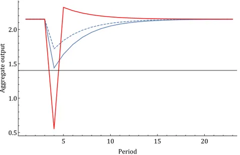
This paper studies the dynamics of an economy relying on collateral reuse subject to aggregate uncertainty that collateral chains might fail. Building on the model of the first chapter, I consider how a shock to collateral chains affects individual reuse decision, collateral allocation and aggregate output. In particular, I contrast outcomes across (i) different temporary shocks and (ii) different persistent shocks, discussing how the size of crisis and the speed of recovery vary with different temporary shocks, and whether a more pro-tracted period of good states will lead to a greater output, or smaller.

As shown in the first chapter, the equilibrium haircut solves incentive prob-lems, and this leads to a wedge between shadow values of the collateral to parties in the collateral chain – for example, if the haircut is positive, the pri-vate value of the collateral to the borrower exceeds the payment, that is, the shadow value of the collateral for the lender. If the loan is over-collateralized, parties down the chain might be tempted to overuse the collateral provided them, and this in turn, causes parties up the chain to be unwilling to ex-tend permission for reuse. In this chapter, I exex-tend this work to a dynamic setting with aggregate uncertainty that collateral chains might fail, deriving the consequences of collateral chain shocks for the re-use decisions and the evolution of the allocation of collateral and aggregate output.

The model highlights the trade-offs of collateral re-use, which are the main driving forces behind the reuse decision making: (1) a positive effect that it helps finance additional productive investments which cannot be financed otherwise by allowing the scarce collateral to support multiple loans at once; (2) a negative effect that it might lead to misallocation of collateral in the event that the intermediary in the middle of the collateral chain defaults. The misallocation of collateral arises from the assumption that collateral is not perfectly liquid in the sense that: (a) the shadow value of collateral is collateral by Goldman Sachs and Merrill Lynch are about 66% and 38%, respectively.

3_{However, there are still differences in the regulation of collateral reuse across countries.}

For example, problems stemming from rehypothecation failure are more severe in Europe than in the US, since in Europe, especially in the UK, there was no limit on the amount that can be rehypothecated by broker-dealers, but in the US, SEC rule 15c3-3 restricts the amount of client assets that can be rehypothecated to no more than 140% of the value of the client’s liability.

(39)

higher for borrowers than for lenders;4 _{and (b) the market for collateral is} not frictionless, so that buying or selling collateral is costly. Combining these two assumptions yields the result that collateral is misallocated in the event that the intermediary fails, since collateral cannot be returned to borrowers who value them highest.

A key variable that determines the relative size of these two trade-off ef-fects is the risk of failure of the intermediary. If the risk of default of the intermediary is lower, the positive effect to finance additional investment is more likely to exceed the negative effect to cause collateral misallocation, so that the initial owner is more likely to extend permission to reuse his collat-eral; and the opposite happens if the risk of default of the intermediary is higher. This implies that given that the risk of failure of the intermediary tends to be counter-cyclical, collateral reuse occurs more frequently in booms than in recessions.

Using this model, I study the effect of shocks that increase the risk of failures of the collateral chain on dynamics of the economy. In particular, I compare outcomes across (i) different temporary shocks and (ii) different persistent shocks. Endogenizing the reuse decisions complicates the charac-terization of the evolution of collateral allocation. As the shock is worse, more collateral cannot be returned to the borrowers, increasing the misallo-cation of collateral, while at the same time, the borrowers are less willing to allow their counterparty to reuse their collateral with concerns of losing the collateral, decreasing the misallocation of collateral. It follows that aggregate output can be even greater after the adverse shock depending on the relative size of these two opposing effects; if the effect of the shock that causes bor-rowers not to allow collateral reuse exceeds the effect that increases failures of returning collateral, the misma

Three essays on economics of rehypothecation