B E F O R E V E N T U R I N G I N T O T H E S U B J E C T O F S A M P L E D E P T H A N D C H R O N O L -

B E F O R E V E N T U R I N G I N T O T H E S U B J E C T O F S A M P L E D E P T H A N D C H R O N O L -O G Y Q U A L I T Y, W E S TAT E F R -O M T H E B E G I N N I N G “ M -O R E I S A L W A Y S B E TT E R ” . H O W E V E R , A S M E N TT I O N E D E A R L I E R O N TT H E S U B J E C TT O F B I O L O G I C A L G R O W T H P O P U L AT I O N S T H I S D O E S N O T M E A N T H AT O N E C O U L D N O T I M -P R O V E A C H R O N O L O G Y B Y R E D U C I N G T H E N U M B E R O F S E R I E S U S E D I F T H E P U R P O S E O F R E M O V I N G S A M P L E S I S T O E N H A N C E A D E S I R E D S I G -N A L . T H E A B I L I T Y T O P I C K A -N D C H O O S E W H I C H S A M P L E T O U S E I S A -N A D V A N TA G E U N I Q U E T O D E N D R O C L I M AT O L O G Y. T H AT S A I D I T B E G S T H E Q U E S T I O N , H O W L O W C A N W E G O ? E S P E R E T A L ( 2 0 0 3 ) , T R E E - R I N G R E S E A R C H 5 9, 8 1 – 9 8 . T H E C O M B I N AT I O N O F S O M E D ATA A N D A N A C H I N G D E S I R E F O R A N A N S W E R D O E S N O T E N S U R E T H AT A R E A S O N A B L E A N S W E R C A N B E E X -T R A C -T E D F R O M A G I V E N B O D Y O F D A-TA . J O H N T U K E Y A N A R T I C L E A B O U T C O M P U TAT I O N A L S C I E N C E I N A S C I E N T I F I C P U B L I -C AT I O N I S N O T T H E S -C H O L A R S H I P I T S E L F, I T I S M E R E LY A D V E R T I S I N G O F T H E S C H O L A R S H I P. T H E A C T U A L S C H O L A R S H I P I S T H E C O M P L E T E S O F T W A R E D E V E L O P M E N T E N V I R O N M E N T A N D T H E C O M P L E T E S E T O F I N S T R U C T I O N S W H I C H G E N E R AT E D T H E F I G U R E S . J O N C L A E R B O U T

C H R I S T O P H E P O U Z AT

S P I K E S O R T I N G : A R E

-P R O D U C I B L E E X A M -P L E

U S I N G R

Copyright ©2010Christophe Pouzat

Contents

Spike Sorting

13

Spike Train Analysis

21

Bibliography

23

Software and Packages Versions

25

List of Figures

1 First400ms of data. 15

2 Filtering / smoothing comparison. 15 3 Events statistics. 16

4 Clean events sample. 16

5 Illustration of number of PCs choice. 17

6 Scatter plots matrix of projections onto planes defined by pairs of

principal components. 18

7 Kmeans results with10centers. 19 8 Median and MAD of kmeans clusters. 20 9 Events from3of the10clusters. 20

List of Tables

1 Elementary spike train statistics of the10isolated units. nb, total

number of spikes; freq, rounded frequency (Hz); min, shortest isi (ms); max, longest isi (ms); mean, mean isi (ms); sd, isis’ SD (ms). Durations rounded to the nearest ms. 21

Introduction

If you are brand new toRread what follows.Ris free, open source and of coursereally great. You can get it from theR projectsite1

. 1

http://www.r-project.org

You will also need another free and open source software: the

GGobi Data Visualization System2

.

2

http://www.ggobi.org/

These two software can seem a bit hard to use at first sight. R

does not follow the nowadays common “point and click” paradigm. That means that a bit of patience and a careful reading of the tuto-rials arede rigueur.Rdocumentation is plentiful and goes from the very basic to the most advanced stuff. The “contributed documen-tation” page3

is good place to start. Look in particular at: “R for 3

http://cran.r-project.org/ other-docs.html

Beginners” by Emmanuel Paradis (french and spanish versions are also available) and “An Introduction to R: Software for Statistical Modelling & Computing” by Petra Kuhnert and Bill Venables4

. 4

Petra Kuhnert and Bill Venables. An Introduction to R: Software for Statistical Modelling & Computing. Technical report, CSIRO Mathematical

and Information Sciences,2005. URL

http://www.csiro.au/resources/ Rcoursenotes.html

Another good place is Ross Ihaka’s course: “Information Visualisa-tion”, the course usesRto generate actual examples of data visual-ization5

and is a wonderful introduction to its subject. Ross Ihaka,

5

http://www.stat.auckland.ac.nz/ ~ihaka/120/

together with Robert Gentleman, is moreover one of the originalR

developers. The “two-day short course in R”6

of Thomas Lumley is

6

You can find it at the following

address:http://faculty.washington.

edu/tlumley/b514/R-fundamentals. pdf.

also great. There is anR Wikisite7

which is worth looking at.

7

http://www.sciviews.org/_rgui/ wiki/doku.php

Windowsusers can enjoy theSciViews R GUIdeveloped by Philippe Grosjean & Eric Lecoutre8

and are strongly encouraged

8

http://www.sciviews.org/ SciViews-R/index.html

to use theTinn-R9

editor to editRcodes, etc. Information on how to

9

http://www.sciviews.org/Tinn-R/ index.html

configureTinn-RandRcan be found in the lecture notes of Kuhnert and Venables. OnLinuxI’m using theemacseditor together with

ESS : Emacs Speaks Statistics 10

.

10

Spike Sorting

At the beginning of this document bothRcommands and there results will be presented. We will then turn to a presentation of the results only as we would do to document our own analysis. But the full set of commands necessary to reproduce it exactly is available in the associatedvignette11

, the “.Rnw” file. 11

Friedrich Leisch. Sweave and Beyond: Computations on Text Doc-uments. In Kurt Hornik, Friedrich Leisch, and Achim Zeileis, editors,

Proceedings of the3rd International Workshop on Distributed Statistical Computing, Vienna, Austria,2003. URLhttp://www.ci.tuwien.ac.at/ Conferences/DSC-2003/Proceedings/.

ISSN1609-395X

We now give a complete example of reproducible research in a spike sorting context. This example make use of a set ofRfunctions calledSpikeOMaticto be released sometime, hopefully soon, as a properRpackage. The present set of functions together with a tutorial can be downloaded from theSpikeOMaticweb page12

. 12 http://www.biomedicale. univ-paris5.fr/physcerv/C_ Pouzat/newSOM/newSOMtutorial/ newSOMtutorial.html.

Starting up

AfterRhas been started by clicking on the proper icon or by typing something like:

$ R

at the terminal (I’m assuming here that the terminal prompt is the symbol $). Since some of the functions we are going to use make use of random initialization it is important, if we want to keep our analysis strictly reproducible, to seed our (pseudo-)random number generator (rng) explicitly. When several choices of rngs are available it cannot hurt to be explicit in our choice. We therefore start by usingset.seedfunction:

> set.seed(20061001,"Mersenne-Twister")

When we deal with long analysis (or with long simulations) storing partial results can save a lot of time while our work progresses. This done by using packagecacheSweaveorpgfSweave13

and by 13

The latter calls the former. defining a sub-directory into which partial results are going to be

stored or cached. This is done with functionsetCacheDir:

> setCacheDir("cache")

Here our partial results are going to be stored in a sub-directory called “cache”.

We keep going by loading the set of functions making upSpikeOMatic

14 s p i k e s o r t i n g: a r e p ro du c i b l e e x a m p l e u s i n g r

> ## Define a common address part

> baseURL <- "http://www.biomedicale.univ-paris5.fr/physcerv/C_Pouzat" > ## Define last part of address to code

> codeURL <- "Code_folder/SpikeOMatic.R"

> ## source code in workspace

> source(paste(baseURL,"/",codeURL,sep=""))

Loading data

The data are freely available from the web14

. They are made of a 14

http://www.biomedicale.

univ-paris5.fr/physcerv/C_Pouzat/ Data.html.

20s long tetrode recording from a locust,Schistocerca americana,

antennal lobe. The data were collected in the absence of

stimula-tion, filtered between300and5000Hz and sampled at15kHz15. 15

Negative potentials appear as up-ward deviations on these data (a re-main of an intracellular physiologist’s past).

They are stored as “native binary” with64bits per measurement

(which is an overkill since the UIE DAQ board used had a16bits

precision). The data are available in compressed format so we first download the4files corresponding to the4recording sites of the

tetrode from the server to our working directory on our hard drive:

> ## Define last part of address to data > dataURL <- "Data_folder/" > ## define dataNames > dataNames <- paste("Locust_",1:4,".dat.gz",sep="") > ## download files > sapply(dataNames, function(dn) download.file(paste(baseURL,"/",dataURL,dn, sep=""), destfile=dn,quiet=TRUE,mode="wb") )

> ## Check that the files are now in working directory > list.files(pattern=".dat.gz")

[1] "Locust_1.dat.gz" "Locust_2.dat.gz" "Locust_3.dat.gz" [4] "Locust_4.dat.gz"

We now load the data intoR’s workspace:

> locust <- sapply(dataNames, function(dn) { myCon <- gzfile(dn,open="rb") x <- readBin(myCon,what="double",n=20*15000) close(myCon) x } )

s p i k e s o r t i n g 15

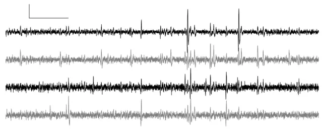
The first400ms of data are shown next.

Figure1_{: The first}400_{ms of data on}

site1_,2_,3_and4_{(from top to bottom)}

of one tetrode. Horizontal scale bar:50

ms; vertical scale bar:500_µV.

Preprocessing

We might want to explore the effect of filtering. A low-pass filter could be applied to eliminate part of the high frequency noise. Smoothing with cubic spline functions with a smoothing parameter set by minimizing thegeneralized cross validationcriterion16 16

B. D. Ripley. Pattern Recognition and

Neural Networks. Cambridge University

Press,1996

could also be used.

Figure2:25ms from the first

record-ing site (middle), smoothed with a

cubic spline (top) and filter with a3

kHz Bessel filter (bottom). The region

shows the first “big” spike of figure1.

For the data at hand neither filtering nor smoothing improves the sorting quality. Smoothing does in fact make it slightly worst due to an apparent extra peak position jitter resulting from the smoothing procedure. We will therefore focus next on the analysis carried out on the raw data. It is nevertheless straightforward to perform the same analysis on the filtered or on the smoothed data by changing one variable name in the.Rnwfile.

Spike detection

Following the precise description given in theSpikeOMatic(new) tutorial we quickly come to the detection step. The detection threshold on each recording site is set as a multiple of the me-dial absolute deviation(MAD) on the corresponding site. Although

SpikeOMaticcontains utility functions likesummaryto help its user setting these thresholds this step is not well automatized requiring decisions to be made by the user. This is one step where the repro-ducible analysis approach is particularly useful since non-automatic actions get fully documented. For the present data, we decided to settle on a threshold of4times the MAD on each recording site.

Only local maxima (peaks) were detected. The detection was more-over performed on a box-filtered version of the data17

. With such a 17

Each measurement is replaced by the average of itself and its two nearest neighbors.

16 s p i k e s o r t i n g: a r e p ro du c i b l e e x a m p l e u s i n g r

Cutting events

Once spikes are detected, events have to be “cut”, that is, a small window is taken from the raw data, on each recording site, around the event’s occurrence time. Then two parameters have to be cho-sen: the window length and the events reference time position within the window. For these data we chose windows of3ms

plac-ing the reference time (peak) at1ms. These two parameters are

again chosen by the user, a choice fully documented in the vignette. A user / reader having access to this vignette (the.Rnwfile) can easily change these parameters at will and see the effect on the final analysis. Time (ms) Amplitude −1 0 1 2 ch1 0.0 0.5 1.0 1.5 2.0 2.5 3.0 ch2 0.0 0.5 1.0 1.5 2.0 2.5 3.0 ch3 −1 0 1 2 ch4

Figure3: The median event (red) and

its MAD (black). Sample size:1723.

Ordinate unit:100_µV.

From this point and for “simple” data like this locust antennal lobe recording, we get our classification of events in a two steps process. When events are defined by3ms long windows and when

several neurons are active in the recording some events will in fact be the result of the near simultaneous occurrence of2or more

action potentials. We would like to identify and classify events due to the superposition of two spikes as such. We will therefore build a “clean” sample by removing from our original sample the most obvious superpositions as shown on the figure bellow. This is done by building an event specific envelope witha singlemaximum and

at most twominima. SpikeOMaticincludes a function allowing users to set interactively the parameters of this envelope (see the tutorial) or to check, interactively again, how good the envelope parameters provided in a vignette are. With this data set, using the envelope

parameters given in the vignette we start with a1679events18large 18

When events get “cut”, if two spikes are within a single window a single one is kept, the largest. This number is therefore smaller than the number of detected spikes.

sample and end up with1472clean events.

Time (ms) Amplitude −5 0 5 10 ch1 0.0 0.5 1.0 1.5 2.0 2.5 3.0 ch2 0.0 0.5 1.0 1.5 2.0 2.5 3.0 ch3 −5 0 5 10 ch4 Time (ms) Amplitude −5 0 5 10 ch1 0.0 0.5 1.0 1.5 2.0 2.5 3.0 ch2 0.0 0.5 1.0 1.5 2.0 2.5 3.0 ch3 −5 0 5 10 ch4 Time (ms) Amplitude −5 0 5 10 ch1 0.0 0.5 1.0 1.5 2.0 2.5 3.0 ch2 0.0 0.5 1.0 1.5 2.0 2.5 3.0 ch3 −5 0 5 10 ch4

Figure4_{: Left, the first}100_events;

middle, the89_{“clean” events; right,}

the11_{“unclean” events.}

Dimension reduction

We are presently using3ms long windows on4recording sites

to represent our events. Since our sampling rate was15kHz our

sample space has 4×15×103×3×10−3 = 180 dimensions. Such a large number can become a serious problem if we try to estimate both location (mean value) and scale (covariance matrix)

s p i k e s o r t i n g 17

parameters of probability densities. Since this is precisely what some of our model-based clustering algorithms are going to do,

we have toreduce the dimension of our sample space before going further. We use systematicallyprincipal component analysis(PCA) to do that. Clearly other methods likeindependent components analysis

(ICA) could be used. Since they are implemented inRa sceptical reader having access to our vignette could very easily try out such an alternative method and see if any different classification would follow. In our experience PCA does a perfectly good job but we have to admit that we are not ICA experts.

Fine but even if you agree that PCA is satisfying there is still a decision to make: How many dimensions (principal compo-nents) should we keep. We don’t believe that an automatic crite-rion like: keep enough components to account for80% of the total

variance, is suitable. The number of components to keep depends too strongly on the signal to noise ratio of the individual neurons spikes and on the number of neurons present in the data. In other words it is too sample dependent19

. So we keepkcomponents if 19

But for a given preparation,e.g.the

locust antennal lobe, we always end up with nearly the same number of components.

the projection of the clean sample on the plane defined by com-ponentskandk+1 is “featureless”, that is, looks like a bivariate Gaussian20

. We point out at this stage that interactive multidimen- 20

See the discussion in Ripley (1996_{) p.}

296_.

sional visualization software likeGGobican be extremly useful in this decision process. We see (bellow) that a “structure” is still ap-parent in the projection of the clean sample onto the plane defined by principal components7and8(left), there is a slight decrease of

points density around -2.5on the abscissa (also visible on the

den-sity estimate shown on the right). No such structure seems present in the projection onto the plane defined by principal components8

and9. -10 _-5 0 5 10 -10 -5 0 5 10 Proj. on PC7 Pr oj. on PC 8 -10 _-5 0 5 10 -10 -5 0 5 10 Proj. on PC8 Pr oj. on PC 9 -10 _-5 0 5 10 0 . 00 0 . 10 0 . 20 Proj. on PC Density estimate

Figure5: Left, clean sample projected

on the plane defined by PC7and8;

middle, clean sample projected on the

plane defined by PC8and9; right,

estimated densities of projections on

PC7(black, smoothing bandwidth:

0.39) and on PC8(grey, smoothing

bandwidth:0.25). A Gaussian kernel

was used for densities estimation. The bandwidth were chosen to slightly undersmooth the data.

Based on these observations we would decide to keep the first

7principal components which happen to account for75% of the

total sample variance. The matrix of scatter plots whose elements are sample projection on the planes defined by every possible pair of principal components already shows nice clusters. We see for instance on figure6 10clusters on the projection onto the plane

de-fined by principal components2and3(second row, third column),

18 s p i k e s o r t i n g: a r e p ro du c i b l e e x a m p l e u s i n g r

our models. Here again using a dynamic visualization software like

GGobican be very useful, since more often than not some structures which are lost on sequences of static projections start appearing clearly. PC 1 −15 −5 5 15 −20 −10 0 5 10 −10 0 5 10 15 −50 −30 −10 0 −15 −5 5 15 PC 2 PC 3 −5 0 5 10 20 −20 −10 0 5 10 PC 4 PC 5 −15 −5 0 5 10 −10 0 5 10 15 PC 6 −50 −30 −10 0 −5 0 5 10 20 −15 −5 0 5 10 −10 −5 0 5 −10 −5 0 5 PC 7

Figure6: Scatter plot matrix of

projec-tions onto planes defined by pairs of

the7principal components. Smooth

density estimates of projections onto the corresponding principal compo-nent are shwon on the diagonal.

Clustering

Since our last graph shows10well separated clusters we can start

with a very simple clustering method likekmeansand run it with10

centers. Doing that we get the clusters shown on figure7.

The median and medial absolute deviation of each of the10

s p i k e s o r t i n g 19 -10 0 10 20 30 -15 -10 -5 0 5 10 15 Proj. on PC3 Pr oj. on PC 2 1 2 3 4 5 6 7 8 9 10

Figure7: Results of kmeans clustering

with10centers projected onto the

plane defined by principle components

2_and3_{. The first}500_{clean events are}

shown.

are all nearly flat and a the same level on each recording site in-dependently of the cluster. This is an indication of both good clas-sificationandof stability of the spike waveform of the individual neurons. In other words the intra-cluster variability is almost en-tirely due to the background noise. When a slight deviation from the horizontal appears on the MAD curves, like for the first and the fourth clusters, it occurs at the point of steepest slope of the mean waveform and is due to uncompensated sampling jitter21

. The over- 21

C. Pouzat, O. Mazor, and G. Lau-rent. Using noise signature to optimize spike-sorting and to as-sess neuronal classification qual-ity. J Neurosci Methods,122(1):

43–57,2002. d o i:10.1016/S0165

-0270(02)00276-5. Pre-print

avail-able at:http://www.biomedicale.

univ-paris5.fr/physcerv/C_Pouzat/ Papers_folder/PouzatEtAl_2002.pdf

all mean value of the medial absolute deviation is65_µV. Inspection

of the mean waveforms and comparison of their peak values with the MAD level suggests moreover that the last three clusters give rise to signals too small for reliable classification.

A conservative approach would be to forget about these last three clusters in the subsequent analysis and consider that only7

good clusters / neurons are present in the data set. Before going further one should of course look at the individual events on a cluster by cluster basis as shown on figure9. This is easily done

withSpikeOMaticand the required commands are present in the associated vignette. UsingGGobiat this stage is also a good idea. Model construction and complete sample classification proceed in a straightforward way as described in the tutorial and explic-itly shown in the vignette. The superposition identification works moreover rather well on this "easy" data set as can be checked with theplotmethod for sorting results ofSpikeOMatic(not shown but directly usable from the vignette).

20 s p i k e s o r t i n g: a r e p ro du c i b l e e x a m p l e u s i n g r Time (ms) Amplitude (mV) -0_.5 0.0 0.5 1_.0 0.0 1.0 2.0 3.0 0.0 1.0 2.0 3.0 0.0 1.0 2.0 3.0 0.0 1.0 2.0 3.0 0.0 1.0 2.0 3.0 -0.5 0_.0 0.5 1.0 -0.5 0_.0 0.5 1.0 0_.0 1_.0 2_.0 3_.0 0_.0 1_.0 2_.0 3_.0 0_.0 1_.0 2_.0 3_.0 0_.0 1_.0 2_.0 3_.0 0_.0 1_.0 2_.0 3_.0 -0.5 0.0 0_.5 1.0

Figure8: The median (black) and

MAD (grey) of the10clusters

ob-tained with kmeans. Cluster number increases from left to right and

cor-respond to the legend of figure7.

Channel1is at the top, channel4at

the bottom. Time (ms) Amplitude −5 0 5 10 ch1 0.0 0.5 1.0 1.5 2.0 2.5 3.0 ch2 0.0 0.5 1.0 1.5 2.0 2.5 3.0 ch3 −5 0 5 10 ch4 Time (ms) Amplitude −5 0 5 ch1 0.0 0.5 1.0 1.5 2.0 2.5 3.0 ch2 0.0 0.5 1.0 1.5 2.0 2.5 3.0 ch3 −5 0 5 ch4 Time (ms) Amplitude −4 −2 0 2 4 ch1 0.0 0.5 1.0 1.5 2.0 2.5 3.0 ch2 0.0 0.5 1.0 1.5 2.0 2.5 3.0 ch3 −4 −2 0 2 4 ch4

Figure9: Left, the36events from

cluster / neuron1; middle, the first50

of the198events from cluster / neuron

7; right, the first50of the215events

Spike Train Analysis

Given the very short duration,20s, of the recording we cannot

illustrate any serious spike train analysis endeavour. We will there-fore stick to some very basic stuff.

nb freq min max mean sd

Neuron1 90 4 22 2828 213 399 Neuron2 89 4 5 1567 224 329 Neuron3 77 4 8 1435 246 303 Neuron4 169 8 15 1075 117 192 Neuron5 132 7 10 1060 147 170 Neuron6 167 8 3 1253 119 169 Neuron7 222 11 0 690 90 123 Neuron8 324 16 2 634 62 65 Neuron9 442 22 1 255 45 44 Neuron10 341 17 2 658 58 68

Table1: Elementary spike train

statis-tics of the10isolated units. nb, total

number of spikes; freq, rounded fre-quency (Hz); min, shortest isi (ms); max, longest isi (ms); mean, mean isi (ms); sd, isis’ SD (ms). Durations rounded to the nearest ms.

Bibliography

Petra Kuhnert and Bill Venables. An Introduction to R: Software for Statistical Modelling & Computing. Technical report, CSIRO Mathematical and Information Sciences,2005. URL_http://www.

csiro.au/resources/Rcoursenotes.html.

Friedrich Leisch. Sweave and Beyond: Computations on Text Documents. In Kurt Hornik, Friedrich Leisch, and Achim Zeileis, editors,Proceedings of the3rd International Workshop on Distributed Statistical Computing, Vienna, Austria,2003. URLhttp://www.

ci.tuwien.ac.at/Conferences/DSC-2003/Proceedings/. ISSN

1609-395X.

C. Pouzat, O. Mazor, and G. Laurent. Using noise signa-ture to optimize spike-sorting and to assess neuronal classifi-cation quality. J Neurosci Methods,122(1):43–57,2002. d o i:

10.1016/S0165-0270(02)00276-5. Pre-print available at: _http:

//www.biomedicale.univ-paris5.fr/physcerv/C_Pouzat/Papers_ folder/PouzatEtAl_2002.pdf.

B. D. Ripley. Pattern Recognition and Neural Networks. Cambridge University Press,1996.

Software and Packages Versions

In order to get real reproducibility when performing an analysis requiring several user contributed packages, one must keep track of theRand user contributed packages version used.

• R version2.11.0(2010-04-22),x86_64-unknown-linux-gnu

• Base packages: base, datasets, graphics, grDevices, methods, splines, stats, utils

• Other packages: cacheSweave0.4-4, class7.3-2, codetools0.2-2,

filehash2.1, getopt1.15, gss1.1-0, lattice0.18-5, MASS7.3-5,

mgcv1.6-2, pgfSweave1.0.5, ppc1.01, R2HTML2.0.0,

STAR0.3-4, stashR0.3-3, survival2.35-8, tikzDevice0.4.8,

xtable1.5-6

• Loaded via a namespace (and not attached): digest0.4.2,

Index

cacheSweave,13

generalized cross validation,15

ICA,17

independent components analysis,

17

kmeans,18

MAD,15,16

medial absolute deviation,15

PCA,17

pgfSweave,13

principal component analysis,17

set.seed,13

setCacheDir,13

summary,15