Estimating Fair Premium Rates for Deposit Insurance Using Option Pricing Theory: An Empirical Study of Japanese Banks

(1)

Estimating Fair Premium

Rates for Deposit Insurance

Using Option Pricing Theory:

An Empirical Study

of Japanese Banks

Nobuyuki Oda

This paper is an expansion and revision of a paper originally submitted to a research conference on “Analyses of Stock Markets Using Financial Engineering Techniques” held by the Bank of Japan in July 1998. The author wishes to emphasize that the content and opinions in this paper are his own and do not necessarily represent the official position of the Bank of Japan.

This paper utilizes option pricing theory to analyze bank stock prices as one method of estimating fair variable deposit insurance premium rates in accordance with individual bank default risk, and conducts empirical analyses using Japanese data.

The purpose of the analyses is to discuss the framework of public organs’ delegate monitoring of bank management. One of the functions of the deposit insurance system is such monitoring. The present system in the United States incorporates the subjective judgment of a bank supervisor combined with certain objective criteria for setting premium rates. There is a need to analyze the types of methodologies that might be viewed as options for adoption in Japan.

To determine whether setting premium rates based on stock price infor-mation is a valid and stable approach, comparative analysis is conducted on the results of trial calculations utilizing this method versus other bank management indexes (credit ratings, etc.), and case analyses are carried out on failed banks. The conclusion is that while this method does involve a certain valuation error, it is an effective means of identifying banks with bad conditions. Moreover, the results confirm that by making adjustments for the changes in market expectations regarding the forbearance of the supervisory authorities, the accuracy of the estimates can be improved. Finally, this paper considers the impact on bank management that could be expected if this method were actually adopted.

Key words: Deposit insurance; Variable deposit insurance rates; Option pricing theory; Stock price; Credit risk; Bankruptcy forecasting; Forbearance

(2)

I. Introduction

This paper examines a method of estimating fair premium rates for deposit insurance (hereinafter referred to as “insurance rates”) in accordance with the default risk on deposits (the bank default risk). Specifically, the examination is centered around empirical analyses of a method of estimating the insurance rates based on bank stock price information utilizing option pricing theory.

Under the present deposit insurance systems in Japan and many other nations, in principle all banks are obligated to subscribe, so a uniform flat insurance rate is charged to all banks regardless of the contents of their portfolios or their manage-ment conditions. The problem with this arrangemanage-ment is that it does not provide sufficient disincentives preventing banks from taking excessive risks in an effort to realize high profit ratios (engaging in high-risk, high-return fund management), even though it is known that this increases the likelihood of default. Despite this flaw, to date the vast majority of deposit insurance systems in most countries have been based on flat insurance rates. Many economists have long argued that insurance rates should be charged in accordance with bank risk, if at all possible (and that a variable insurance rate system should be introduced to this end). Among economists, the debate is whether or not it is possible for third parties (i.e., investors, analysts, regulatory authorities including deposit insurance organs, etc.) to accurately grasp the contents of banks’ assets (market prices and risk).

This paper examines the option pricing theory approach, which is considered to be a strong candidate method for the estimation of fair insurance rates, by analyzing the estimation results for Japanese banks. There are no clear criteria for judging the accuracy of the estimated insurance rates, and it is difficult to test statistically. Nevertheless, various aspects of this issue are considered herein, including compara-tive analyses with other information related to the status of bank management as well as case analyses of failed financial institutions. While this paper takes the approach of analyzing problems with deposit insurance systems, from another perspective one might say that it also examines the issue of the extent to which the information included in bank stock prices (the information context) reflects the actual conditions of bank management.

This paper is organized as follows. Prior to beginning the actual analyses of insur-ance rates, Chapter II examines and summarizes the original functions of deposit insurance and discusses the insurance rate systems actually being used in Japan and the United States. Chapter III presents methodologies for estimating insurance rates using the option pricing theory approach: the Merton method, the Marcus and Shaked method, and the Ronn and Verma method. Chapter IV reports the results of the empirical analyses, and this represents the core of this paper. These analyses can be broadly divided into estimations of the insurance rates given the forbearance expectations, and estimations of the insurance rates after estimating the expectations themselves. Finally, Chapter V presents some concluding remarks.

(3)

II. Functions of Deposit Insurance and Review of Present

Systems

A. Functions of Deposit Insurance

Prior to addressing the issue of deposit insurance premium rates, this section reviews the functions and roles of deposit insurance.1

In a number of nations, deposit insurance is operated on a monopoly basis directly by the government or by government-affiliated organs rather than by private-sector insurance companies, and in many cases the banks are obligated to subscribe. Thus, deposit insurance may be interpreted as a type of government intervention in the banking industry. In general, government intervention is deemed justified when an appropriate allocation of resources cannot be realized by relying exclusively on the free market (so-called “market failures”). In the case of deposit insurance, because there is an extremely large asymmetry in information between the banks and the depositors (especially small-lot depositors), from the standpoint of the social costs involved, it is considered inappropriate for the depositors to personally monitor the management conditions of the banks and select where they will deposit their funds in accordance with the principle of self-accountability. Accordingly, from the perspec-tive of economics, the primary justification for the existence of deposit insurance is the delegate monitoring function whereby the government (deposit insurance organ) monitors the status of bank management on behalf of the depositors.2 _Moreover, based on the results of this monitoring, the government should then take appropriate action on behalf of the depositors.3

Then what types of actions are appropriate for governments to pursue based on the results of monitoring the management conditions of banks? Theoretically, if one were to make the major assumption that governments have complete access to all information and can accurately judge the status of bank management in all cases without fail, the goal could be achieved simply by having the government announce whether each individual bank’s management conditions are sound, and there would be no need to set risk-adjusted variable insurance rates. (This is because if governments had access to all information, no risk would occur in the first place.) In practical terms, however, there is a certain asymmetry of information between

1. The contents of this section are not limited to ideas for which a general consensus has been reached, but also include the personal opinions of the author.

2. The protection of small-lot depositors is often cited as the objective of deposit insurance. In line with the logic of this paper, the act of reducing the possibility that depositors may unintentionally deposit their funds in banks with poor management conditions itself may be interpreted as the protection of depositors.

Additionally, the function of guaranteeing deposits by such actions as paying off depositors in the unlikely event of bank failure may also be viewed as having the function of depositor protection. In this paper, however, this is considered as part of the post-failure disposal process, and does not constitute the primary purpose of deposit insurance.

It is also a fact that in Japan and other nations the present deposit insurance systems sometimes fulfill certain roles in maintaining the stability of the financial system and conducting appropriate disposal of failed financial institutions. However, this paper makes a clear distinction between such roles and the original functions of deposit insurance, and does not address these types of ancillary functions.

3. In addition to deposit insurance, types of intervention whereby the government monitors banks on behalf of the depositors and takes appropriate action include early resolution and prompt corrective action. The question of which approach represents the optimal system is an important issue, but it lies outside the scope of this paper.

(4)

governments and the banks, and governments must accept a certain level of judg-ment error (risk) in their assessjudg-ments of bank managejudg-ment conditions.4_Considering this point, for example, just as institutional investors demand a risk premium when they invest in bonds, governments should also demand risk premiums from each bank on behalf of the depositors. Based on the assumption that the government’s risk monitoring cost would be lower than that for monitoring by each individual deposi-tor, the premium demanded by the government would be less than the premium demanded by depositors if there were no deposit insurance, so from a macroeco-nomic standpoint the social cost would be reduced. Considering this argument in light of the purpose of deposit insurance, the implication is that fair insurance rates should be set for each bank in accordance with the individual bank risk.

Can fair insurance rates therefore be set based on the subjective evaluation of the government (evaluations via bank inspections, etc.)? The answer to this question depends on two factors. First, is the information held by the government absolutely superior to that held by other parties? This paper makes the a priori assumption that while the government holds information that is not available anywhere else, market prices also incorporate information that the government has not taken notice of, and thus government and market information are mutually complementary. Second, even assuming that the information held by the government is absolutely superior, the problem is that there is no guarantee that the discretionary policy decisions will always incorporate optimal conclusions. While this paper does not enter into a theo-retical examination of this point, as one intuitive example, the government may have some incentive to monitor the situation for a while and give the banks a chance to revive themselves rather than simply liquidating failed banks. (When failed banks successfully recover financial soundness, the government averts the danger of having its responsibility for supervising banks called into question.) One means of com-pensating for this latent bias is to incorporate certain objective evaluation standards or rules (such as evaluation based on stock prices, which is the main subject of this paper, or evaluation based on capital adequacy ratios, which is adopted in the United States) in the process of setting insurance rates, instead of leaving this to the discretion of government authorities.

Keeping the above reasoning in mind, the following sections examine the validity of using stock price information and option pricing theory as one method of objective evaluation.

B. Prior Research on Variable Deposit Insurance Rates

A great deal of research has been conducted on ideal deposit insurance systems. This section presents a brief introduction to a few papers that consider the setting of variable insurance rates.

To begin with, there are basically two opinions as to whether the government has access to sufficient information to set fair, risk-adjusted insurance rates. The first position is that, because the government cannot gain access to the private 4. The fact that the problem of moral hazard is frequently cited under flat insurance rate systems suggests that there

(5)

information held by banks, in practice it is not possible to make accurate judgments of banks’ management conditions. Among researchers who accept this premise, some believe that by constructing mechanisms that satisfy incentive compatible constraints, it would be possible to achieve the same effect as by charging risk-adjusted insurance rates.5 _{The second position is that by effectively utilizing all types of information} the government can, to some extent, effectively grasp the management conditions of banks. In this case, the main concern is how to set risk-neutral insurance rates (a system in which the relative size of the insurance rates corresponds to the relative size of the risk), or how to set fair insurance rates (a system in which the absolute level of the insurance rates corresponds to the absolute level of the risk).6 _{The topic} of this paper, estimating fair insurance rates using option pricing theory based on bank stock price information, belongs to the latter line of thought.

The following chapter introduces three papers from the United States on methods for calculating insurance rates using option theory (the Merton method, the Marcus and Shaked method, and the Ronn and Verma method). First, let us examine three Japanese research papers that employ these calculation methods. In what is con-sidered the first Japanese paper regarding this theme, Omura (1986) employs the Merton method, calculates fair insurance rates for 13 city banks as of September 1985, and compares them with the insurance rate charged in Japan at that time (a flat rate of 0.012 percent). Ikeo (1991a, b) calculates fair insurance rates for 53 of Japan’s nationwide banks at two points in time—the end of September 1985 and the end of March 1986—based on the Ronn and Verma method, and argues that on average the actual rate charged (0.012 percent) functions as a subsidy (that is, on average the rate charged is too low compared with the fair rates).7 _{Most recently,} (while they do not estimate fair insurance rates), Saito and Moridaira (1998) utilize the framework of the Merton method to calculate the probability that banks will fall into a net debt position. Specifically, they estimate the probabilities of 119 banks falling into a net debt position on a daily basis from April 1995 through March 1998, and conduct analyses on the transition of these probability figures.

In contrast with these earlier research efforts, the main distinctive characteristics of the empirical analysis in this paper (Chapter IV) may be summarized as follows. (1) The Ronn and Verma method is adopted, and the estimations also make

adjustments for the forbearance expectations effect (Section IV.C).

(2) The fair insurance rates are estimated at the individual bank level and, although this is anecdotal, considerations are also given to the validity of the estimates (Section IV.B).

(3) A practical perspective is adopted as consideration is given to the types of administration that could realistically be used if this method were actually incorporated into Japan’s deposit insurance system (Section IV.D).

(4) The analysis period is long term, covering the post-“bubble” era from the end of March 1990 through the end of March 1998 (Section IV.B).

5. For example, refer to Chan, Greenbaum, and Thakor (1992).

6. Refer to Iwamura (1992) for a discussion of risk-neutral insurance rates and fair insurance rates.

7. Ikeo (1991a, b) assumed, a priori, that the value of the forbearance expectations parameter ρ, which is explained in chapters III and IV of this paper, is 0.97. This paper expands on this point, and attempts to estimate the fair insurance rates after estimating the value of ρitself.

(6)

C. Current Deposit Insurance Rates in Japan and the United States

This section presents an outline of the deposit insurance rate systems currently used in Japan and the United States as preliminary information prior to the analyses using actual data in Chapter IV.

1. Deposit insurance rates in Japan

In Japan, the deposit insurance system covers banks,8 _{shinkin banks, credit} coopera-tives and labor credit associations with headquarters located in Japan. Deposits are insured for up to ¥10 million in principle per financial institution for funds deposited in the types of accounts that are insured.9 _{Through March 1996, all} financial institutions were charged a flat insurance rate of 0.012 percent as a general insurance premium, but from April 1996 the insurance rate has been 0.048 percent as a general insurance premium plus 0.036 percent as a special insurance premium,10 for a total premium rate of 0.084 percent.

2. Deposit insurance rates in the United States

In the United States, Section 302(a) of the Federal Deposit Insurance Corporation Improvement Act of 1991 (hereinafter referred to as the “FDICIA”) mandated the introduction of risk-related premiums, and these have actually been applied since 1994.11_{As shown in Table 1, the core of this system is the classification of banks into}

8. City banks, regional banks, member banks of the Second Association of Regional Banks, trust banks, long-term credit banks, etc.

9. The types of accounts insured are current-account deposits, ordinary deposits, deposits at notice, deposits for tax payments, saving deposits, time deposits, installment savings, special deposits, installments, and money in trust with guaranteed repayment of principal (including loans in trust), as well as installment asset accumulation products utilizing the above-mentioned types of accounts. Foreign currency deposits and negotiable certificates of deposit are not covered by the insurance system.

10. The special insurance premium is a temporary measure that will expire in fiscal 2000.

11. For an outline of the FDICIA and considerations on Japanese financial system, refer to Okina (1993), for example. Table 1 Deposit Insurance Premium Rates in the United States (Fiscal 1996)

Basis points

Supervisory groups Bank Insurance Fund (BIF)

Healthy Supervisory_concern Significant super-_{visory concern}

Capital Well capitalized 0 3 17

adequacy Adequately capitalized 3 10 24

Undercapitalized 10 24 27

Savings Association Supervisory groups

Insurance Fund (SAIF) Healthy Supervisory_concern Significant super-_{visory concern}

Capital Well capitalized 23 26 29

adequacy Adequately capitalized 26 29 30

Undercapitalized 29 30 31

Note: The capital adequacy categories are defined by a combination of three criteria: (1) the capital (Tier 1) adequacy ratio under the Basle Agreement; (2) the capital (Tier 1 + Tier 2) adequacy ratio under the Basle Agreement; and (3) the leverage ratio (the capital [Tier 1 + Tier 2] divided by total assets). Financial institutions are categorized as “well capitalized” when (1) is at least 6.0 percent, (2) is at least 10.0 percent, and (3) is at least 5.0 percent. Financial institutions are categorized as “adequately capitalized” when (1) is at least 4.0 percent, (2) is at least 8.0 percent, and (3) is at least 4.0 percent. Financial institutions are categorized as “undercapitalized” when (1) is less than 4.0 percent, (2) is less than 8.0 percent, or (3) is less than 4.0 percent.

(7)

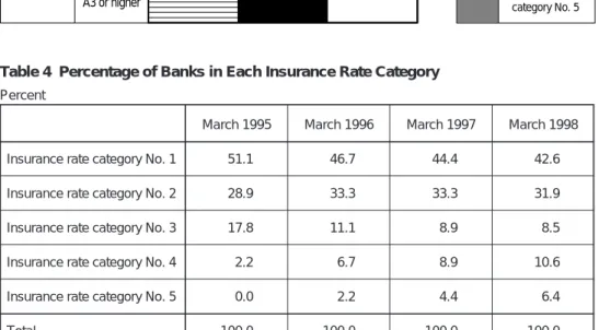
a total of nine risk categories by capital adequacy (three categories) and the evaluation of the supervisory authority (three categories) together with the setting of different insurance rates for each risk category.12_{The insurance rates charged for each category} may be revised (in fact, the premiums were revised twice [downward] between the time the system was first applied in January 1994 and the time the rates shown in Table 1 were implemented). At present, the vast majority of financial institutions are rated in the top risk category (“well capitalized” under the capital adequacy ratings and an “A” evaluation from the supervisory authority). Specifically, as of the end of 1996, 95.0 percent of the institutions were placed in the top risk category by the Bank Insurance Fund (BIF), and 89.9 percent were placed in this category by the Savings Association Insurance Fund (SAIF). Thus, only a small number of institutions presently fall into the eight other risk categories.

III. Methods for Calculating Fair Premium Rates for Deposit

Insurance Using Option Pricing Theory

This chapter presents a summary of three methods for calculating fair insurance rates13 _{applying option pricing theory: (1) the Merton method (Merton [1977]);} (2) the Marcus and Shaked method (Marcus and Shaked [1984]); and (3) the Ronn and Verma method (Ronn and Verma [1986, 1989]). Method (2) may be considered as an improved version of method (1), and method (3) may be considered as an improved version of method (2). The empirical analyses in Chapter IV utilize method (3).

A. Merton Method

Merton (1977) adopts the Black-Scholes option pricing theory for the calculation of fair insurance rates, as follows. From the viewpoint of the body providing deposit insurance, the required cash flow G at the time of maturity T of the insured bank’s liabilities (for simplification, a single type of discount bond is assumed) may be defined as follows.

G = max (0, B – V ). (1)

Here, V is the value of the bank’s assets and B is the face value of the bank’s liabilities. Consequently, G expresses the bank’s net liabilities, and the deposit insurance is obligated to cover this. Taking B as a constant and V as a stochastic variable, equation (1) may be interpreted as expressing the payoff on a European put option where the value of the bank’s assets V is the underlying asset and the face value of the bank’s liabilities B the exercise price. Therefore, in determining the value of insurance, assuming that the value of the bank’s assets V follows a lognormal process 12. According to the Federal Deposit Insurance Corporation (1997).

13. For terminological convenience, estimated insurance rates using option pricing theory based on bank stock price information are referred to as “fair insurance rates.” (Of course, further examinations would be required to determine whether or not the estimation results are really fair.)

(8)

(with a volatility of σv), the option theory pricing equation (the Black-Scholes formula) can be applied. In this case, the fair insurance premium P may be calculated as follows. P = Be–rT_{N (x +}σ v√T ) – VN (x ) B 1 (2) 1n — – (r + –– σv2)T V 2 where x≡————————— . σv√T

Here, r expresses the risk-free interest rate.14 _{The function N (•) is the cumulative} probability density function for a standard normal distribution. In equation (2),

V and σv are unknowns, and the fair insurance rates can be determined by seeking

their values.

B. Marcus and Shaked Method

Marcus and Shaked (1984) make certain revisions to the Merton method and conduct empirical analyses on U.S. bank stock price data.

As for the computational method, the Marcus and Shaked method differs from the Merton method in two ways. First, Marcus and Shaked note that the value of bank assets differs before and after a bank obtains deposit insurance. Specifically, they define V as the value of bank assets before the bank obtains deposit insurance. If P is the value of the deposit insurance, then the value of the bank assets after the bank obtains deposit insurance may be expressed as V + P. Marcus and Shaked assume that

V is a stochastic variable that follows a lognormal process (with a volatility of σv), and

using equation (1) as a starting point the value of the deposit insurance P (the fair insurance rate) can be derived by applying the Black-Scholes formula as follows.

P = Be–rT_{N (x +}σ v√T ) – Ve–δTN (x ) B 1 (3) 1n — – (r – δ+ –– σ2 v)T V 2 where x≡—————————— . σv√T

Here, B is the face value of the bank’s liabilities, r is the risk-free interest rate, and the function N (•) is the cumulative probability density function for a standard normal distribution. Equation (3) is basically equivalent to equation (2), but inasmuch as equation (3) clearly incorporates the effect whereby internal reserves decrease through stock dividend distributions (the dividend rate is defined as δ), it is a generalized version of equation (2).

14. Under the Merton method, the result includes the risk-free interest rate but does not include the risk premium because in asset valuation theory with no arbitrage condition the return on a risk-free composite portfolio must equal the risk-free interest rate. In contrast, some analysts (such as Moridaira [1997]) argue that because there are no securities or markets for trading in the asset values V of banks (or more broadly, of corporations) themselves, it is inappropriate to further develop this line of reasoning, and that the expected growth rates of the assets or some other factor should be used in place of the risk-free interest rate. However, it should also be noted that in practice it is difficult to estimate risk premiums or the expected growth rates of assets.

(9)

The second point in which the Marcus and Shaked method differs from the Merton method is as follows. Marcus and Shaked note that equation (2) includes two unknowns that cannot be directly observed (that is, the value of the bank’s assets V and the volatility of this variable σv), and introduce the following two relations so that these unknowns can be estimated. The first equation is

V + P = D + E. (4)

Here, D is the present value of the bank’s liabilities and E is the present value of the bank’s capital (total equity). Equation (4) may be interpreted as a general relation showing the balance between assets, liabilities, and capital. In the Merton method, for simplification, a single type of discount bond is assumed for the liabilities, but here general bonds are assumed and different variables are given for the face value B and the present value D. Of course, in actual computations some sort of relationship must be assumed between B and D. By assuming a bond that pays a risk-free interest rate r , Marcus and Shaked assume the case in which the present value of the bond is equal to the face value of the bond, as follows.

V + P = B + E. (4')

The second relation is

∂E

σEE = σvV —— ._∂ (5)

V

This is the result of applying Ito’s lemma (known in stochastic calculus), noting that the present value of the bank’s capital E is a stochastic variable dependent on the value of the bank’s assets V and its volatility σv (that is, E = E (V, σv). Here σE indicates the volatility of the present value of the bank’s capital E. To rearrange equation (5), first equation (3) is substituted into equation (4).

E = V – D + P (6)

= V – D + Be–rT_{N (x +}σ

v√T ) – Ve–δTN (x ).

By substituting equation (6) and its differential form into equation (5), the result is

Be–rT_{[1 – N (x +}σ v√T )]

σv= σE

{

1 – ——————————

}

. (7)

Ve–δT_{[1 – N (x )]}

Then the three unknowns P, V, and σv can be calculated by simultaneously solving equations (3), (4'), and (7). In seeking a numerical solution to these simulta-neous equations, the book value is used for the face value of the bank’s liabilities B, and the present value of the bank’s capital E is calculated by multiplying the stock price by the total number of outstanding ordinary shares. The volatility of E (σE) is estimated from past stock price data.

(10)

Using this equation, Marcus and Shaked calculated the fair insurance rates for 40 major U.S. banks between 1979 and 1980, and compared these with the rates actually being charged by the FDIC (the effective premium rate was 0.077–0.083 percent after adjusting for the effect of rebates). Their conclusion was that the fair rates would be less than one-half of the rates charged by the FDIC, even after accounting for the FDIC’s operating costs, implying that the FDIC was overpricing its deposit insurance.

C. Ronn and Verma Method

Ronn and Verma (1986, 1989) use the framework of the Marcus and Shaked method with several modifications.

Specifically, the Ronn and Verma method has two points in common with the Marcus and Shaked method. First, Ronn and Verma express the fair insurance rate as the premium on a put option using the Black-Scholes formula. Second, because the bank’s asset value and its volatility cannot be observed directly, they estimate these figures using data on stock prices and stock price volatility, which can be observed. On the other hand, the Ronn and Verma method differs from the Marcus and Shaked method in the following four ways. First, they adopt the asset value after the bank obtains deposit insurance as the underlying asset for the option that determines the fair insurance rate (in this section, this is referred to as V, and it should be noted that this definition of V differs from that adopted in Section B above), and assume that this V is a probability variable that follows a lognormal process. Second, in accordance with this expression, equation (4) in the Marcus and Shaked method can be rewritten as V = D + E, but Ronn and Verma do not adopt this relationship, and instead assume the following relationship.

E = VN (y ) – ρBN (y – σv√T ) V 1 (8) 1n

[

——

]

+ ––σ2 vT ρB 2 where y≡——————— . σv√T

This is consistent with Black and Scholes (1973), who demonstrated that a corporation’s (here, a bank’s) capital value can be estimated using the theoretical price of a call option (the underlying asset is the asset value V and the exercise price is the future value of the bank’s debt BerT_{, where B is the face value of the bank’s debt).} However, in equation (8), as the exercise price, BerT _{is multiplied by}ρ_{(0 <}ρ ≤ _1), and this is the third difference from the Marcus and Shaked method. This takes account of the common understanding that when a bank falls into a net debt position, the supervisory authorities (here the FDIC) may sometimes provide financial assistance or otherwise exercise forbearance15 _{rather than ordering an} immediate bank closure. Under this model, a bank closure is not ordered at the 15. Ronn and Verma (1986) use the phrase “a temporary reprieve from closure,” but here the word “forbearance”—

(11)

moment when V equals B (when the bank falls into a net debt position). Rather, the bank closure is only ordered when V declines to ρB (≤B ). Consequently, the

parameter ρ may be interpreted as expressing the market expectations of the possibility of financial assistance and/or forbearance by the supervisory authorities (hereinafter, these are referred to as “forbearance expectations”). Ronn and Verma conduct most of their numerical analyses at ρ= 0.97. Also, Ronn and Verma report that while changing the value of ρnaturally changes the absolute amount of each bank’s deposit insurance rate, this results in virtually no change to the relative amounts of the insurance rates charged to different banks. Like Marcus and Shaked, Ronn and Verma also utilize the relation in equation (5), but by rearranging the equation, instead of the expression in equation (7), they derive the following equation.

σEE

σv= ——— . (9)

VN (y )

This is the result of substituting ∂E/∂V = N (y ), which is the result of a partial

differentiation of equation (8), into equation (5).

Finally, the fourth difference versus the Marcus and Shaked method is that the framework of the Ronn and Verma method includes both insured liabilities (face value B1) and uninsured liabilities (face value B2≡B – B1). They use the situation in

which all of the liabilities (face value B ) are covered by the deposit insurance. At this point, the hypothetical deposit insurance premium P' is calculated in the same way used in the Marcus and Shaked method.

P' = BN (x + σv√T ) – Ve–δTN (x ) B 1 (10) 1n — + (δ– –– σ2 v)T V 2 where x≡————————— . σv√T

Because just B1/B percent of the total liabilities are actually covered by the deposit

insurance, assuming that the seniority of all the liabilities is equal, the deposit insurance premium P is calculated as follows.

B1 P = — P' B Ve–δT_B 1 (11) = B1N (x + σv√T ) – ——— N (x ). B

This can then be converted into the insurance rate d as follows.

P d ≡— B1 Ve–δT (12) = N (x + σv√T ) – ——— N (x ). B

(12)

Using the above results, first the unknowns V and σv can be calculated by simultaneously solving equations (8) and (9).16 _{The fair insurance rate can then be} determined by substituting the results into equations (11) and (12).

IV. Empirical Analyses

In this chapter, fair insurance rates are estimated following the Ronn and Verma method using stock price data for Japanese banks. The chapter includes considera-tions of the technical issues regarding the estimation method and an evaluation of the validity of the estimation results, as well as an examination of the effects that might be expected if this type of rate structure were actually adopted for the Japanese deposit insurance system.

In principle, the objects of the analyses are limited to city banks, long-term credit banks, trust banks, regional banks, and member banks of the Second Association of Regional Banks that have adopted the international standards (1988 Basle Agreement) for disclosure of the capital adequacy information (a total of 87 banks).17 As necessary, however, some analyses only cover banks that have received credit ratings (Moody’s long-term deposit ratings), and the chapter also includes case analyses of failed banks. The data used are the stock prices at the end of each Japanese fiscal year,18 _{the outstanding number of shares, total liabilities,}19 _{and the}

16. Iteration is used to solve these simultaneous equations in accordance with the following procedure. First, two new variables are defined for convenience.

a≡y b≡y – σv√T .

(FN.1) The relationships between these new variables and the unknowns may be expressed as follows.

a – b σv= ——— √T (FN.2) a2_{– b}2 V = ρB exp (———). (FN.3) 2

Then the binary simultaneous equations derived from equations (8) and (9) are rewritten using a and b as follows.

σEE√T a = ————— + b (FN.4) ρBN (b ) + E a – b a2_{– b}2 ——ρBN (a )exp (———) – σEE = 0. (FN.5) √T 2

If equation (FN.5) is solved for a and b using the Newtonian method with equation (FN.4) as a condition of constraint, by substituting the results into equations (FN.2) and (FN.3), the values of the unknowns can then be determined.

17. These include some banks that previously adopted the international standards (1988 Basle Agreement) but now follow domestic Japanese standards. However, institutions that were already bankrupt by March 1997 are not included.

18. In this chapter, the stock prices at the end of each fiscal year are always used for calculating the insurance rates for each fiscal year. To realize a more stable evaluation for the actual management of the system, however, the use of the average stock prices during each fiscal year might be considered. Nevertheless, this issue is not considered in this paper.

19. In these analyses, the book values of the liabilities are adopted as approximations of the present values. Under the financial accounting for Japanese banks, however, the incidental credits and debts “acceptances and guarantees” and “customers’ liability for acceptances and guarantees” are recorded in the nominal capital, and the present values of these items differ greatly from the book values (the nominal capital). To address this issue, in this paper “liabilities” are defined as the book value of total liabilities minus “acceptances and guarantees.”

(13)

historical volatility calculated from the daily stock prices in the applicable fiscal year (the standard deviation of the daily rate of return). The longest analysis period extends from the end of fiscal 1989 (March 1990) through the end of fiscal 1997 (March 1998), and thus the analyses cover a period in which Japanese stock prices fluctuated substantially.

A. Handling of Parameters for the Analyses

In applying the Ronn and Verma method presented above (Section III.C), two parameters need to be set: the option period T when the stock prices are interpreted as options, and the market expectations of supervisors’ forbearance ρ.

1. Setting of the option period

As for the option period T, taking the hypothetical case in which the liabilities of the banks being evaluated all have the same maturity, the equity value may be interpreted as the liquidation value following the period T, so T corresponds to the liability maturity. In actual practice, however, bank liabilities are comprised of numerous liabilities with different maturities, and it is difficult to set the value of T based on maturity information. In this paper, making reference to prior research, the value of T is set a priori at one year, and this value is used consistently throughout the analyses. Ronn and Verma (1986) report on how the fair insurance rates are influenced by the value of T. Their research shows that while the value of T has a substantial influence on the absolute amount of each bank’s deposit insurance rate, this results in virtually no change to the relative amounts of the insurance rates charged to different banks. Consequently, the decision to set the value of T at one year in this paper does not represent any impediment to a relative evaluation of the fair insurance rate for each bank.

2. Setting of the forbearance expectations

The next issue is the setting of the forbearance expectations parameter ρ. This paper assumes that the value of ρis the same for all banks at any given point in time (that is, the supervisory authorities do not discriminate among banks in terms of forbear-ance), and adopts two approaches. The first approach is to assume that the value of

ρ does not change over time, and (similar to the approach used for the value of T above) to adopt a fixed value a priori. In this case, (as in the discussion of T above) this approach is deemed valid for a cross-sectional relative valuation of fair insurance rates. However, in conducting relative valuation in a time series, this approach is limited to cases in which the forbearance expectations do not change over time. This approach is adopted throughout the multifaceted analyses in Section B of this chapter to determine whether or not fair insurance rates based on stock prices are valid indicators.

The second approach is to use new external information, and then estimate the implied value of ρ based on this. In this paper, the average spread on debentures by rating level is noted, and the value of ρ is estimated to minimize, overall, the gap between each bank’s fair insurance rates and this spread. The details of this logic and the analysis results are presented in Section C of this chapter.

(14)

B. Estimation of Fair Premium Rates for Deposit Insurance 1. Influence of forbearance expectations

In this section, a fixed value is adopted for the forbearance expectations parameter ρ, and the validity of the resulting estimates of fair insurance rates is examined. Before entering into the empirical analyses, let us first examine how the estimation results change as a result of adopting different values for ρ.

Figure 1 shows the estimation results for fair insurance rates at the end of fiscal 1996 for banks rated by Moody’s by rating level. The value of ρis set at six different levels: 0.90, 0.93, 0.95, 0.97, 0.99, and 1.00. The figure shows that different values for ρresult in very little change to the relative amounts of the insurance rates charged to different banks. Thus, setting a fixed a priori value for ρdoes not represent a prob-lem for the examination in this chapter of whether it is possible to set insurance rates that reflect the relative likelihood of each bank’s default. Here, the value of ρis set at 0.9720_{to roughly approximate the rates currently charged under the Japanese deposit} insurance system (0.048 percent as a general insurance premium plus 0.036 percent as a special insurance premium, for a total premium rate of 0.084 percent). The analysis period for this section runs through March 1997 (it does not include the figures from the end of March 1998). The estimation of an appropriate level for the value of ρis discussed in Section C below.

2. Regarding the validity of the estimates: examinations using cross-sectional data

One of the key points of this research is to examine whether fair insurance rates estimated from stock prices using option pricing theory accurately reflect the actual default probability of banks. In Japan, however, because only a small number of banks have defaulted in the past, it is difficult to verify this statistically. As an alter-native, this paper adopts three relative variables other than fair insurance rates that indicate the management conditions at each bank: (1) capital adequacy; (2) danger points, which are defined21 _{based on the “total points” for the overall bank ranking} presented annually in the journal Kin’yu Bijinesu (Financial Business) published by

Toyo Keizai Shimposha; and (3) credit ratings (Moody’s long-term deposit ratings). As

a basic approach in making the comparisons, as with the deposit insurance premium rate system used in the United States (as explained in Section II.C), it is considered effective to use a mutually complementary combination of subjective and objective judgments for the evaluation of each bank. The first choice for a subjective judgment would be the inspection and examination results of the supervisory authorities, but because this is not disclosed to the public (2) the danger points and (3) the credit ratings are adopted for the analyses as alternatives. As for objective judgments, (1) capital adequacy (which is also used in the United States) and the fair insurance rate (which is the main theme of this research) are utilized.

20. The value of ρwas also set at 0.97 in previous research in the United States and Japan (Ronn and Verma [1986], Ikeo [1991b]), so this facilitates direct comparisons with these research efforts.

21. The “total points” for the overall bank ranking are calculated based on various management and financial indexes, and the higher the number of “total points,” the better the bank management conditions. In this paper, to facilitate comparison with other variables, the differentials versus the highest number of “total points” awarded in each fiscal year are defined as “danger points,” and under this conversion the higher the number of “danger points,” the worse the bank management conditions.

(15)

0.0 1 2 3 4 5 6 7 8 9 Percent

Aaa Aa1 Aa2 Aa3 A1 A2 A3 Baa1 Baa2 Baa3

Estimated fair insurance rate

Credit rating 0 0.5 1.0 1.5 2.0 2.5 3.0 3.5 Percent

Credit rating 0 1 2 3 4 5 6 7 8 9 Percent

Credit rating

Figure 1 Fair Insurance Rates Estimated with Different ρValues [1] ρ= 0.90

[2] ρ= 0.93

(16)

0.0

Credit rating 0.5 1.0 1.5 2.0 2.5 3.0 3.5

Percent

[4] ρ= 0.97

Credit rating 0.00 0.01 0.02 0.03 0.04 0.05 0.06 0.07 0.08 0.09

Percent

[5] ρ= 0.99

Credit rating 0.00 0.01 0.02 0.03 0.04 0.05 0.06 0.07 0.08 0.09

Percent

(17)

To start with, capital adequacy categories are adopted as the objective judgment, and the relationships of these to the danger points and the credit ratings (as subjec-tive judgments) are presented in figures 2 and 3, respecsubjec-tively. The capital adequacy categories adopted here follow the system used for setting deposit insurance premium rates in the United States.22

Figures 2 and 3 show a wide dispersion of both the danger points and the credit ratings, essentially regardless of the capital adequacy categorization results (well capi-talized, adequately capicapi-talized, or undercapitalized). Thus, judging from these data alone, the use of Japanese capital adequacy ratios appears to be insufficient.23

Next, fair insurance rates are adopted as the objective judgment, and the relation-ships versus the danger points and the credit ratings (as subjective judgments) are presented in figures 4 and 5, respectively. As an overall trend, figures 4 and 5 show a positive correlation between the fair insurance rates and the subjective evaluations at all points in time. Thus, the objective and subjective evaluation methods may be considered as consistent overall. At the individual bank level, however, there are a few cases in each figure where the evaluation based on fair insurance rates is not consistent with the subjective evaluation. For example, in Figure 4 the danger points of banks No. 53 and No. 54 are relatively harsh while the evaluations based on fair insurance rates are relatively good. Conversely, in Figure 4 the danger points of banks No. 75, No. 76, and No. 77 are relatively good while the evaluations based on fair insurance rates are relatively harsh. While the judgments may vary substantially in certain cases depending upon the evaluation criteria adopted, as long as there are not too many divergences, there is a possibility that the objective and subjective evalua-tion methods may be mutually complementary, with each method compensating for the weak points in the other.

22. The capital adequacy categories adopted here are defined by a combination of three criteria: (1) the capital (Tier 1) adequacy ratio under the Basle Agreement; (2) the capital (Tier 1 + Tier 2) adequacy ratio under the Basle Agreement; and (3) the leverage ratio (the capital [Tier 1 + Tier 2] divided by total assets). Here, financial institutions are categorized as “well capitalized” when (1) is at least 5.0 percent, (2) is at least 9.0 percent, and (3) is at least 3.5 percent. Financial institutions are categorized as “adequately capitalized” when (1) is at least 4.0 percent, (2) is at least 8.0 percent, and (3) is at least 3.0 percent. Financial institutions are categorized as “undercapitalized” when (1) is less than 4.0 percent, (2) is less than 8.0 percent, or (3) is less than 3.0 percent. The boundary values separating the three categories have been set for the convenience of this analysis, and do not necessarily match those adopted by the deposit insurance system in the United States, as presented in Chapter II. (Considering the differences between the systems in Japan and the United States, for the purposes of this research it is convenient to set boundary values that differ from each other.)

23. In the future, however, Japanese capital adequacy ratios may become more significant with the adoption of accounting systems that more accurately reflect actual risk, such as incorporating the results of internal audits.

(18)

31 30 36 27 9 35 74 83734 55 17 41 28 45 25 5 38 32 48 24 66 47 65 61 80 70 49 43 44 64 87 71 62 68 67 73 82 59 72 60 69 63 58 86 16 3 39 1 7 23 57 26 2 77 76 78 19 6 4 14 ₇₉ 18 50 83 56 75 40 29 46 81 51 33 10 22 15 21 42 0 500 1,000 1,500 2,000 2,500 3,000 3,500 4,000 4,500 Capital adequacy Well capitalized Adequately capitalized Danger points Under-capitalized 31 30 36 27 ₉ 35 74 83734 55 17 41 28 45 25 5 38 32 48 24 66 47 65 61 80 70 49 43 44 64 87 71 62 68 67 73 82 59 72 60 69 63 58 86 16 3 39 1 7 23 57 26 2 77 76 78 19 6 4 14 79 18 50 83 56 75 40 29 46 81 51 53 54 33 84 10 22 15 21 42 0 500 1,000 1,500 2,000 2,500 3,000 3,500 4,000 4,500 Danger points Capital adequacy Well capitalized Adequately capitalized Under-capitalized 31 30 36 27 9 35 74 8 37 34 55 17 41 28 45 25 5 38 32 48 24 66 47 65 61 80 70 49 43 44 64 87 71 62 68 67 73 82 59 72 60 69 63 58 86 16 3 39 1 7 23 57 26 2 77 76 78 19 6 4 14 79 18 50 83 56 75 40 29 46 81 51 53 54 33 84 85 20 10 22 15 21 42 0 500 1,000 1,500 2,000 2,500 3,000 3,500 4,000 4,500 Danger points Under-capitalized Well capitalized Adequately capitalized Capital adequacy

Figure 2 Capital Adequacy versus Danger Points [1] End of March 1997

[2] End of March 1996

(19)

36 11 30 13 12 9 35 8 55 17 28 5 32 47 65 49 43 44 62 59 60 63 58 16 3 39 1 7 57 26 2 19 6 4 14 18 50 56 40 29 46 51 10 15 Aaa Aa1 Aa2 Aa3 A1 A2 A3 Baa1 Baa2 Baa3 Moody’s rating Capital adequacy Well capitalized Adequately capitalized Under-capitalized 36 11 30 13 12 9 35 8 55 17 28 5 32 47 65 49 43 44 62 59 60 63 58 16 3 39 1 7 57 26 2 19 6 4 14 18 50 56 40 29 46 51 10 15 Aaa Aa1 Aa2 Aa3 A1 A2 A3 Baa1 Baa2 Baa3 Moody’s rating Under-capitalized Well capitalized Adequately capitalized Capital adequacy 36 11 30 13 12 9 35 ₈ 55 17 28 5 32 47 65 49 43 44 62 59 60 63 58 16 3 39 1 7 57 26 2 19 6 4 14 1850 56 40 29 46 51 20 10 15 Aaa Aa1 Aa2 Aa3 A1 A2 A3 Baa1 Baa2 Baa3 Moody’s rating Capital adequacy Well capitalized Adequately capitalized Under-capitalized

Figure 3 Capital Adequacy versus Credit Ratings [1] End of March 1997

(20)

31 30 36 279 35 74 837 3455 17 41 28 4525 5 38₃₂48 24 6647 65 61 80 70 49 43 44 6487 71 62 6867 73 825972 6069 63 58 86 16 3 39 17 2357 26 2 77 76 78 19 6 4 14 79 18 50 8356 75 40 29 46 81 51 53 54 33 8452 85 20 10 22 15 21 42 0 500 1,000 1,500 2,000 2,500 3,000 3,500 4,000 4,500 0 0.2 0.4 0.6 0.8 1.0 1.2 1.4 Danger points

Estimated fair insurance rate (percent)

31 30 36 279 35 74 8 37 34 55 17 41 28 45 25 5 3832 48 246647 65 61 80 70 49 4344 64 87 71₆₂ 68 67 73 82 59 72 6069 63 58 86₁₆ 3 39 1 7 23 57 26 2 77 76 78 19 6 4 14 79 18 50 83 56 75 40 29 46 81 51 53 54 33 84 52 85 20 10 22 15 21 42 0 500 1,000 1,500 2,000 2,500 3,000 3,500 4,000 4,500 0 0.1 0.2 0.3 0.4 0.5 0.6 0.7 0.8 Danger points

31 30 36 27₉ 35 74 8 37 34 55 17 41 28 45 25 5 38 32 48 24 66 47 65 6180 70 49 43 44 64 87 71 62 68 67 73 82 59 72 60 69 63 58 86 16 3 391 7 23 57 26 2 77 76 7819 6 4 14 79 18 50 83 7556 40 29 46 81 51 53 54 33 84 52 85 20 10 22 15 21₄₂ 0 500 1,000 1,500 2,000 2,500 3,000 3,500 4,000 4,500 0 0.1 0.2 0.3 0.4 0.5 0.6 0.7 0.8 Danger points

Figure 4 Estimated Fair Insurance Rates versus Danger Points [1] End of March 1997

(21)

36 11 30 13 12 9 35 8 5517 28 5 32 47 6549 43 4462 59 60 63 58 16 3 39 17 57 26 2 19 6 4 14 18 50 56 40 29 4651 20 10 15 0 0.6 1.0 1.4 Aaa Aa1 Aa2 Aa3 A1 A2 A3 Baa1 Baa2 Baa3 0.2 0.4 0.8 1.2 Moody’s rating

36 11 30 13 12 9 35 8 55 17 28 5 32 47 65 49 43 4462 59 60 63 58 16 3 39 1 7 57 262 19 6 4 14 18 50 56 40 2946 51 20 10 15 0 0.2 0.4 0.6 0.8 Aaa Aa1 Aa2 Aa3 A1 A2 A3 Baa1 Baa2 Baa3 0.1 0.3 0.5 0.7 Moody’s rating

36 11 30 13 12 9 35 8 55 17 28 5 32 47 65 49 43 4462 59 60 63 58 16 3 39 1 7 57 26 2 19 6 4 1418 50 56 40 29 46 51 20 10 15 0 0.2 0.4 0.6 0.8 Aaa Aa1 Aa2 Aa3 A1 A2 A3 Baa1 Baa2 Baa3 0.1 0.3 0.5 0.7 Moody’s rating

Figure 5 Estimated Fair Insurance Rates versus Credit Ratings [1] End of March 1997

(22)

3. Regarding the stability of the estimates: examinations using time-series data

As combining fair insurance rates with subjective evaluations has demonstrated a certain validity, this section addresses the stability of the estimates of the fair insurance rates. Out of the 87 banks analyzed for this research, six banks with relatively large fluctuations in the rates between the end of fiscal 1989 and the end of fiscal 1996 are selected, and the time-series transitions of their rates are presented in Figure 6.

Looking at the results, one distinctive characteristic is that when volatility is calculated using the same method adopted in figures 1–5, that is, based on daily stock price data over a one-year period (shown by the dotted lines in Figure 6), the rate for each bank is conspicuously high at the end of fiscal 1992, protruding from the prior and subsequent figures. As the stock price levels were not unusually low at the end of fiscal 1992 (refer to Figure 9 below), one may surmise that this was caused by the volatility level.24_{When the rates are revised calculating the volatility based on} the daily stock price data over a half-year period (shown by the solid lines in Figure 6), the jump seen in the dotted lines virtually disappears. The implication from this example is that the method25 _{used to calculate the volatility may have a significant} influence on the estimated rates.

Along these lines, the shaded bars in Figure 6 indicate the size of fluctuation in the rates shown by the solid lines in Figure 6, and the portion of this that may be attrib-uted to changes in stock prices is indicated by the bars that are not shaded. (Alternatively, one may interpret the difference between the shaded bars and the unshaded bars as the contribution to the rate fluctuations from volatility.) To make an overall judgment regarding this, it should be noted that when the individual bank rates change significantly (such as at the end of fiscal 1996 for banks No. 10, No. 12, and No. 13), the contribution from changes in stock prices is relatively large, and that the majority of what appears to be evaluation “blur” may be attributed to changes in volatility. Of course, the causes of volatility fluctuations include bank disclosure poli-cies, but there is a strong probability that other noise factors may also exert a significant influence. While it is inappropriate to form a general conclusion regarding the scale of this type of “blur” from a limited sample, based solely on the data here a “blur” of over 1.0 percent appears to be rare. Thus, if the estimated rate exceeds 1.0 percent, there is a strong possibility of management instability factors that cannot be explained by noise alone.26_{Conversely, in many cases rate changes of 0.1–0.2 percent can be attributed to} evaluation “blur.” The implication that may be derived from these points is that in order to derive stable rates, the use of some sort of filter may be effective (such as 24. To verify this conjecture, Nikkei Stock Average data for the one-year period from April 1992 through March

1993 indicate that the market was highly volatile during the first half of fiscal 1992 (a volatility of 35.6 percent during the first half), but that the market volatility subsided during the second half (a volatility of 19.2 percent during the second half). Thus, there is a substantial gap between the volatility for the full fiscal year (28.7 percent) and that for the second half (19.2 percent).

25. Strictly speaking, the volatility that should be considered here is the future predicted volatility, but this paper does not address technical means to improve the accuracy of volatility forecasts (for example, the possibility of utilizing the ARCH/GARCH model, etc.), and simply adopts the historical volatility over a set period as the future prediction for the analyses.

26. It should be noted that the 1.0 percent standard being discussed here will change depending upon the value of the forbearance expectations parameter ρ. In other words, the 1.0 percent level is meaningful when the value of ρis set at 0.97, as in this section.

(23)

–0.10 –0.05 0.00 0.05 0.10 0.15 0.20 0.25 1990 91 93 95 96 0 0.05 0.10 0.15 0.20 0.25 92 94 Percent Percent

Changes in the rates (left scale) [obs. period for σ = 0.5 year]

Fair rates (right scale) [obs. period for σ = 0.5 year] Changes in the rates

attributed to changes in stock prices (left scale) [obs. period for σ = 0.5 year]

Fair rates (right scale) [obs. period for σ = 1.0 year]

End of fiscal year

–0.08 –0.06 –0.04 –0.02 0.00 0.02 0.04 0.06 0.08 0.10 0 0.01 0.02 0.03 0.04 0.05 0.06 0.07 0.08 0.09 0.10 1989 90 91 92 93 94 95 96 Percent Percent

Fair rates (right scale) [obs. period for σ = 0.5 year] Changes in the rates (left scale) [obs. period for σ = 0.5 year]

Changes in the rates attributed to changes in stock prices (left scale) [obs. period for σ = 0.5 year]

End of fiscal year

–0.1 0.00 0.1 0.2 0.3 0.4 0.5 0.6 0.7 0.8 0.9 1989 90 91 92 93 94 95 96 0 0.2 0.4 0.6 0.8 1.0 1.2 1.4 Percent Percent

Fair rates (right scale) [obs. period for σ = 0.5 year] Changes in the rates (left scale)

[obs. period for σ = 0.5 year]

Changes in the rates attributed to changes in stock prices (left scale) [obs. period for σ = 0.5 year]

End of fiscal year

Figure 6 Estimated Fair Insurance Rates for Selected Banks and Decomposition of Their Changes [1] Bank No. 2

[2] Bank No. 8

(24)

–0.1 0.00 0.1 0.2 0.3 0.4 0.5 1989 90 91 92 93 94 95 96 0 0.1 0.2 0.3 0.4 0.5 0.6 Percent Percent

Changes in the rates (left scale) [obs. period for σ = 0.5 year] Changes in the rates

attributed to changes in stock prices (left scale) [obs. period for σ = 0.5 year]

End of fiscal year

[4] Bank No. 13 –0.06 –0.04 –0.02 0.00 0.02 0.04 0.06 0.08 0.10 0.12 0.14 0.16 0 0.05 0.10 0.15 0.20 0.25 1989 90 91 92 93 94 95 96 Percent Percent

Fair rates (right scale) [obs. period for σ = 0.5 year] Changes in the rates (left scale)

[obs. period for σ = 0.5 year] Changes in the rates attributed to changes in stock prices (left scale) [obs. period for σ = 0.5 year]

End of fiscal year

[5] Bank No. 16 –0.08 –0.06 –0.04 –0.02 0.00 0.02 0.04 0.06 0.08 0.10 0.12 0.14 0 0.1 0.2 0.3 0.4 0.5 0.6 0.7 0.8 0.9 1989 90 91 92 93 94 95 96 Percent Percent

Changes in the rates (left scale) [obs. period for σ = 0.5 year]

Changes in the rates attributed to changes in stock prices (left scale) [obs. period for σ = 0.5 year] Fair rates (right scale)

End of fiscal year Fair rates (right scale)

(25)

setting several range categories and charging a constant rate for each category). For example, following the analysis here, banks with estimated rates less than about 0.2 percent might be charged a low fixed rate (such as 0.0 percent) considering the likeli-hood of evaluation error, and banks with estimated rates of 1.0 percent or higher might be charged a different fixed rate (such as 1.0 percent) considering the likelihood of some sort of management instability factor. The issues regarding the application of this sort of system are discussed further in Section D below.

4. Case analyses of failed banks

Up until this point, the analysis has mostly covered banks that are still operating. In this section, fair insurance rates are estimated for five banks (all previously listed on Japan’s stock exchanges) that have gone bankrupt. These rates are presented in Figure 7. The last point on the line for each bank corresponds to the time just before that bank failed (the banks all failed within one year from this point in time). At these points, the estimated rates for four of the five banks are over 1.0 percent, and the rate for the fifth bank is over 0.6 percent. Moreover, unusually high rates are seen not only just before the banks failed, but also one or two years prior. Four of the five banks show rates of at least 0.5 percent, and the rate for the fifth bank is over 0.4 percent. Thus, Figure 7 demonstrates that there were warning signs regarding the stability of these banks at least two years before they declared bankruptcy.

If the data for the ends of fiscal years 1996, 1995, and 1994 are plotted onto the figures for each fiscal year in Figure 4 above, only one other bank (Bank No. 85)27 shows rates higher than those of the five banks plotted in Figure 7. Thus, although

0.0 0.2 0.4 0.6 0.8 1.0 1.2 1.4 1.6 1.8 2.0 1989 90 91 92 93 94 95 96 Percent

End of fiscal year Bank No. 92

Bank No. 10 Bank No. 89 Bank No. 90 Bank No. 91

Figure 7 Movements of Estimated Fair Insurance Rates for Failed Banks

27. While Bank No. 85 did not fail in terms of falling into a net debt position, it was announced in May 1998 that the bank was subjected to a “special merger” (in October 1998) under the terms of the Deposit Insurance Law, and that all members of the Board of Directors with the right of representation were to resign. Thus, the management conditions at Bank No. 85 differ from those at all the other banks that are still operating.

(26)

this is ex post facto analysis, in almost every case it was possible to distinguish the banks that failed from those that did not at least one to two years prior to the bank failures.

C. Fair Premium Rates for Deposit Insurance Based on Estimations of Forbearance Expectations

1. Necessity of estimating forbearance expectations

In Section B, ρ is set at a fixed value of 0.97 and fair insurance rates are estimated through the end of March 1997 (the end of fiscal 1996). Here, leaving the value of ρ at 0.97, the fair insurance rates are estimated for all 87 banks through the end of March 1998 (the end of fiscal 1997). The results are presented in Figure 8.

Figure 8 shows that the estimated rates for many of the banks increased sharply over the one-year period through the end of March 1998. Does this indicate that the banks’ management conditions and the contents of their assets suddenly deteriorated (or that the deterioration suddenly became clear) during this one-year period? Intuitively, it seems that some other factor is required to explain such a remarkable change. One possibility is that this development might be due to a change in market participants’ expectations of forbearance by the supervisory authorities. To verify this, the upper chart in Figure 9 presents the daily data of the Bank Stock Price Index (Tokyo Stock Exchange) and the Nikkei Stock Average from April 1, 1996 through April 28, 1998. Several of the conspicuous declines in the Bank Stock Price Index correspond to announcements of bank failures or of radical restructuring plans

0.0 0.2 0.4 0.6 0.8 1.0 1.2 1.4 1.6 1.8 2.0 1990 91 92 93 94 95 96 97 Percent

End of fiscal year

Figure 8 Movements of Estimated Fair Insurance Rates for 87 Banks

(27)

0 5,000 10,000 15,000 20,000 25,000 0 100 200 300 400 500 600 700 800 900 0 5,000 10,000 15,000 20,000 25,000 30,000 35,000 1988 89 90 91 92 93 94 95 96 97 0 200 400 600 800 1,000 1,200 1,400 Nikkei Stock Average (yen) Bank Stock Price Index (yen) End of month Nikkei Stock Average (yen) Bank Stock Price Index (yen)

End of fiscal year 1996

Mar. June Sep. Dec.

97

Mar. June Sep. Dec.

98 Mar. Bank Stock Price Index (right scale) Nikkei Stock Average (left scale) Bank Stock Price Index (right scale) Nikkei Stock Average (left scale)

Note: The upper chart contains daily data from April 1, 1996 to April 28, 1998. The lower chart contains end-of-fiscal-year data from fiscal 1988 to 1997.

Figure 9 Movements of the Bank Stock Price Index and the Nikkei Stock Average including the curtailment of business activities, that is to say, periods when the supervisory authorities took harsh measures toward banks suffering from poor management conditions. (These include the announcements of restructuring at Nippon Credit Bank and the planned merger of Hokkaido Takushoku Bank in

(28)

early April 1997 as well as announcements concerning the failures of Kyoto Kyoei Bank, Hokkaido Takushoku Bank and Tokuyo City Bank in October–November 1997.) Thus, there is a strong likelihood that the forbearance expectations did in fact change.

2. Estimation of forbearance expectations

If the changes in forbearance expectations (deduced above) are significant, as discussed in Section A above, it is necessary to estimate the value of the forbearance parameter ρat each point in time and then to calculate the fair insurance rates using these values of ρ. In this section, the value of ρis estimated using historical data for the bond spread by credit rating.

The basic assumption for this estimation is that, although credit rating data are inferior to stock price data at the individual bank level, they are relatively inde-pendent from forbearance expectations. Thus, credit rating data are effective for judging the average management conditions when placing many banks into sets. In other words, bank stock price data incorporate more information than rating data about management conditions at the individual bank level, but the problem is that bank stock price data also incorporate changes in forbearance expectations. If one accepts that the stock market pricing mechanism is rational and efficient, then this assumption is natural.

The specific procedure for estimating the value of ρ is as follows. First, the fair rates are calculated for all banks rated by Moody’s at the end of each fiscal year for six different values of ρ (1.00, 0.99, 0.97, 0.95, 0.93, and 0.90). Second, based on historical data for the bond spread by rating (as shown in Table 2),28 _{the average} spread over Aaa bonds is calculated for each rating.29_{Noting the differential between} the fair rates for each bank calculated above and the average spread for each corre-sponding rating, the sum of the squares for each differential is sought for each value of ρ, and the results are presented in Table 3. The final step is to seek the values of

ρ that minimize the sum of the squares at each point in time. In this analysis, as an approximation, a quadratic function is applied to the value of ρ (from among the six values of ρ) that results in the smallest sum of the squares and to the two values on both its sides (these three figures are shown in the shaded areas of Table 3) to estimate ρmin, which minimizes the sum of the squares.

The results indicate that the forbearance expectations increased slightly during the one-year period from the end of March 1996 through the end of March 1997 (the increase in ρmin was 0.007), but then increased sharply during the one-year

period from the end of March 1997 through the end of March 1998 (the increase in

ρminwas 0.022, about three times the increase during the previous year).

28. The bond spread data used here (Table 2) are taken from the historical data presented by Cantor, Packer, and Cole (1997). These are the average spreads for 4,399 U.S. bond issues from January 1983 through July 1993 (the ratings used are from both Moody’s and Standard & Poor’s).

29. The bond spread is composed of the expected loss and the risk premium. Because the fair insurance rates covered in this analysis correspond to the expected loss, for comparison the risk premium must be subtracted from the bond spread. This analysis assumes that the risk premium is approximately uniform without referring to the rating, and that the Aaa bond spread is essentially the same as the risk premium (in other words, the expected loss on bonds rated Aaa is zero). As a result, it is possible to compare the average spread over Aaa bonds for each rating with the estimated fair insurance rates.

(29)

3. Fair premium rates for deposit insurance based on estimations of forbearance expectations

Here, new calculations are made for a portion of the analyses conducted in Section B utilizing the ρminvalues estimated above. The ρmin values from Table 3 are used in

place of ρ= 0.97 for the data from the end of fiscal 1994 (March 1995) through the end of fiscal 1997 (March 1998), which are presented in Figure 8 above. The results are presented in Figure 10. In this figure, the changes in the rates for each bank from the end of fiscal 1996 to the end of fiscal 1997 show both increases and decreases, avoiding the extreme results in Figure 8, where almost all of the rates declined. As there is no method to directly verify whether the results in Figure 8 or those in Figure 10 more closely approximate “truly fair insurance rates,” to some extent this must be left up to the subjective judgment of individuals (or of the supervisory authorities or other groups that may have access to superior information).30_{In terms of the changes} in management conditions over this one-year period, however, it appears that the results in Figure 10 are more accurate.

Aaa 0.478 0.000 Aa1 0.637 0.159 Aa2 0.678 0.200 Aa3 0.755 0.277 A1 0.836 0.358 A2 0.879 0.401 A3 1.066 0.588 Baa1 1.196 0.718 Baa2 1.228 0.750 Baa3 1.551 1.073 Ba1 2.128 1.650 Ba2 4.373 3.895 Ba3 3.369 2.891 B1 4.407 3.929 B2 4.526 4.048 B3 4.962 4.484

Credit rating Spread (percent)

Over treasury yield Over Aaa yield

Table 2 Average Bond Spread by Credit Rating

Table 3 Sum of Squares for Each Differential between the Estimated Fair Insurance Rate and the Average Spread by Rating

ρ 1.00 0.99 0.97 0.95 0.93 0.90 ρmin

End of March 1995 16.21 16.13 14.45 8.99 30.09 322.19 0.956

End of March 1996 19.23 19.07 16.45 9.57 28.74 292.39 0.955

End of March 1997 20.28 19.87 14.60 15.25 81.62 557.63 0.962

End of March 1998 16.56 14.32 15.32 53.78 211.63 915.36 0.984

Note: ρminis defined as the ρvalue that minimizes the sum of squares.

30. For example, by examining the correlation between the rates for each bank shown in Figure 10 and management information about the individual banks, it might be possible to confirm the accuracy of the estimation results. However, this paper does not enter into any analyses of microeconomic information concerning the individual banks.