Efficient Computation of Renaming Functions for
ρ-reversible Discrete and Continuous Time Markov Chains
Matteo Sottana
University Ca’ Foscari Venice
[email protected]
Carla Piazza
University of Udine
[email protected]
Andrea Albarelli
University Ca’ Foscari Venice
[email protected]
ABSTRACT
With the introduction of ρ-reversibility, the basic notion of reversible Markov chain has been relaxed by allowing a wider range of scenarios. Specifically, the reversibility prop-erties are not just sought on the chain itself, but also on all the possible topology-preserving renamings of its state space. Such renamings, calledRenaming Functions, exhibit many interesting properties which can be exploited in differ-ent contexts. Unfortunately, finding a renaming function for a Markov chain is a very computationally intensive task. Us-ing a naive approach it could require to check for all the pos-sible state space permutations, which is unfeapos-sible for all but the most trivial chains. As a matter of fact, we prove that the corresponding decision problem is polynomially equiv-alent to Graph Isomorphism. Nevertheless, we introduce an algorithm that, exploiting some necessary conditions for ρ-reversibility, is able to efficiently prune the search space and then verify the remaining renaming candidates. The correctness of the method is theoretically demonstrated and its practical effectiveness is shown over a significant set of discrete and continuousρ-reversible Markov chains.
Keywords
Reversibility modulo Renaming, Discrete and Continuous Time Markov Chains, Algorithms
1.
INTRODUCTION
Markov chains have been widely used to study the per-formance of computer systems and software architectures. In the past decades several formalisms have been developed with the goal of allowing a stochastic model to be speci-fied in a compact way by using features such as composi-tion and hierarchical approaches. Despite the availability of compact representations, a stochastic process does not nec-essarily admits an efficient analysis. For instance, even a simple high-level model may suffer from the so called state space explosion problem that makes the computation of the
Permission to make digital or hard copies of all or part of this work for personal or classroom use is granted without fee provided that copies are not made or distributed for profit or commercial advantage and that copies bear this notice and the full cita-tion on the first page. Copyrights for components of this work owned by others than ACM must be honored. Abstracting with credit is permitted. To copy otherwise, or re-publish, to post on servers or to redistribute to lists, requires prior specific permission and/or a fee. Request permissions from [email protected].
c
2017 ACM. ISBN . DOI:10.1145/1235
steady-state numerically intractable. Discrete and contin-uous time Markov processes are the basis for modeling a wide range of real-world contexts, ranging from chemical re-action dynamics to economic models and computer systems. The analysis of the Markov process underlying this kind of systems, allows us to derive the performance indices of the model, and thus of the modeled system itself. These are often computed at the steady-state (if it exists), when the time elapsed from the initial instant tends to infinity.
The analysis of Markov chains, both at continuous and discrete time, can in many cases be simplified by applying techniques based upon: internal symmetries, for instance re-versibility [6, 8]; state aggregation, such as lumpability [9, 5]; composition, like product forms [2, 3]. Most of such sim-plifications can be exploited in order to allow the numerical or analytical tractability of the computation of performance indices, related by the common concept of time-reversibility. The time-reversibility of Markov stochastic processes has been introduced for the first time and applied to the analysis of stochastic networks and Markov chains by Kelly [6]. A time-reversible Markov process has the property that the process we obtain by reversing the direction of time has the same probabilistic behavior of the original one.
Applications of these results have led to the character-ization of product-form solutions for queuing models with underlying time-reversible Markov chains. Product-form so-lutions allow the study of the sub-components of a system, reducing the state space, and then obtain the metrics of the whole system by computing the product of the metrics of all the sub-components. In particular the product-form theory allows for the derivation of the steady-state distribution of a system as the normalized product of the steady-state dis-tributions of the system’s sub-components, each considered in isolation and opportunely parametrized.
However, time-reversibility is a very restrictive condition since it requires the chain to exhibit definitely the same stochastic behavior presented by its reverse. Indeed, this is a quite rare event and it happens only for a narrow class of chains, thus limiting the aptness of simplification and analy-sis approaches. In order to broaden the scope, a more flexible definition, calledρ-reversibility, has been proposed in [10, 8]. A Markov process is said to beρ-reversible if it is stochas-tically identical to its reversed process modulo a renaming of the state space. The availability of arenaming function
making a chainρ-reversible allows, for instance, the efficient computation of the stationary probabilities or to easily de-compose a process to characterize them as a product form.
Contribution. The main contributions of this paper are two algorithms for testing theρ-reversibility of both DTMCs and CTMCs. The first is a linear time procedure that can be used to test whether a given renaming is valid for a process. The second one exploits the first and solves the more gen-eral problem of finding all renaming functions of a process. Of course, its computation can be stopped as soon as the first valid renaming is produced. The problem —in its deci-sion verdeci-sion— is equivalent to Graph Isomorphism, provided that the stationary distribution has been exactly computed. Despite this complexity result, our algorithm proves its ef-fectiveness on both synthetic and real-world examples. The key ingredients of its efficiency are two necessary conditions that in polynomial time prune the set of possibly valid re-namings. To the best of our knowledge there was no previous feasible approach to solve this problem and the naive check of all the possible maps would require a number of verifica-tion steps which is factorial with respect to the size of the state space.
Related work. In [6] the author deeply discusses the no-tion of time reversibility both for DTMCs and CTMCs, and several applications are illustrated. Dynamic reversibility is introduced in [14] as a tool for the study of physical sys-tems such as the growth of two dimensional crystals. An exploration of the relations among different definitions of lumpability and the notion of time-reversed Markov chain can be found in [10]. The idea of ρ-reversibility is intro-duced for the first time in [8] and its applications in the em-bedded and uniformized chains of continuous time processes are discussed. In [7] the authors introduce the definition of auto-reversibility that allows one to exploit the symmetrical structures of a class of CTMCs to derive the steady-state probabilities in an efficient way. In [9] the authors propose the idea of using a general permutation of states for com-paring forward and reversed processes at continuous time. A review covering the main results regarding time-reversible Markov processes and a discussion about how to apply them to tackle the problem of the quantitative evaluation of re-versible computations can be found in [1]. In [4] the authors show new results on both reversed stationary Markov pro-cesses as well as Markovian process algebra. A connection between exact lumping and time reversibility is proposed in [13]. Finally, in [12] the authors focus on the problem of defining quantitative stochastic models for concurrent and cooperating reversible computations.
Structure of the paper. The remainder of this paper is organized as follows. Section 2 briefly recalls the general no-tions about Markov chains and supplies the definition and notation for both reversibility andρ-reversibility that will be used throughout the following sections. Section 3 discusses in depth the conditions for a Markov chain to beρ-reversible at the basis of our algorithm and studies the complexity of theReversibility modulo Renaming decision problem and its relation with Graph Isomorphism. Section 4 introduces the algorithm we propose for recovering all the feasible re-naming functions mapping a Markov chain to its reversible isomorphic form. Its correctness and complexity are also discussed. In Section 5 the performance and effectiveness of this novel algorithm are demonstrated by applying it to both continuous and discrete Markov chains representing re-spectively synthetic examples and processes related to a real case study. Finally, Section 6 concludes the paper.
2.
SETTING THE CONTEXT
In this section, we briefly recall some basic notions about discrete and continuous time Markov chain. For more details the reader should refer to [6].
2.1
Markov Chains
A discrete time stochastic process X(t) is a sequence of random variables taking values in state space S fort ∈Z.
Similarly, acontinuous time stochastic process X(t) is a se-quence of random variables taking values in state space S
fort∈R. In this paper we will only deal with finite state
spaces. A stochastic process isstationary if it has the same distribution for all timet. AMarkov Chain is a stochastic process such that for allt1<· · ·< tn< tn+1it holds that
P(X(tn+1) =xn+1|X(t1) =x1, . . . , X(tn) =xn) =
P(X(tn+1) =xn+1|X(tn) =xn)
i.e., the past evolution does not influence the conditional probability of the future behaviour. If X(t) is a discrete (continuous) time stochastic process, then the Markov Chain is a Discrete Time Markov Chain (DTMC) (Continuous Time Markov Chain (CTMC), respectively). A Markov chain is said to betime homogeneousif the conditional probability P(X(t+τ) =j|X(t) =i) does not depend upont.
In the case of time homogeneous DTMC for eachi, j∈ S
we use the notation
P(X(t+ 1) =j|X(t) =i) =pij
The valuepijdenotes the probability that the chain, when-ever in statei, next makes a transition into statej, and is referred to as(one-step) transition probability. The square matrix P = (pij)i,j∈S is called(one-step) transistion
ma-trix, and since when leaving stateithe chain must move to one of the statesj∈ S, each row sums to one (i.e., forms a probability distribution).
In the case of time homogeneous CTMC for eachi, j∈ S
and for eacht≥0 we use the notation
P(X(s+t) =j|X(s) =i) =pij(t)
This value represents the probability that the chain from state iaftert time instants ends up in statej. Hence, we can consider the square matricesP(t) = (pij(t))i,j∈S, where P(0) =Idis the identity matrix. It is possible to prove that
dP(t)
dt =QP(t), withQ= dP(t)
dt (0) = (qij)i,j∈S Qis theinfinitesimal generator, all its rows sum to 0 and its diagonal elements are negative. Intuitively, qij with i6=j represents the transition rate from i to j. Given Q the CTMC is completely defined, sinceP(t) =etQ.
A Markov chain isirreducible if every state in S can be reached from every other state. A state in a Markov pro-cess is called recurrent if it is guaranteed that the process will eventually return to the same state (the probability of going back to the state is one). A recurrent state is called
positive-recurrent if the expected number of steps until the process returns to it is finite. A Markov chain isergodic if it is irreducible and all its states are positive recurrent. An ergodic Markov chain has a uniquesteady-state distribution
(stationary distribution), i.e., a distribution of probability π = (πi)i∈S which remains invariant with respect to time.
In the case of DTMC this means that
π=πP (1)
Similarly, in the case of CTMC the meaning is that π = πP(t), for allt≥0,which can be proven to be equivalent to
πQ= 0 (2)
Eq. (1) and (2) are calledGlobal Balance Equations (GBE). In general, the knowledge of the steady-state for a process modeling a system is a key information in order to com-pute its performance indeces, such as throughput, expected number of customers at a queue, admission rates and many others.
2.2
Reversibility
The most obvious method to obtain π is, of course, by solving algebraic problems (1) and (2). However, this ap-proach could suffer from ill-conditioning or numerical insta-bility, since it requires either an iterative computation or a possibly large number of substitutions. Luckily the analysis of ergodic Markov chains can be greatly simplified if the be-havior of the chain remains the same when the direction of time is reversed.
Definition 1 (Reversibility [6]). A processX(t) is reversibleif X(t) and XR(t) =X(τ−t) are stochastically identical for allτ.
It is easy to see that reversible processes are stationary. Moreover, ifX(t) is a Markov chain, thenXR(t) is a Markov chain too. Hence, in the rest of this paper we will consider only ergodic stationary Markov chains.
A characterization of reversibility over (egodic stationary) DTMC is given by the following result.
Theorem 1 (Detailed balance [4]). A DTMCX(t)
defined byPis reversible iff there is a distribution of prob-abilityπ= (πi)i∈S such that for eachi, j∈ S it holds that:
πipij=πjpji (3)
The stationary distribution of bothX(t) andXR(t) isπ. The above theorem can be exploited to efficiently compute the stationary distribution of reversible processes. The same result holds for CTMCs replacingPwithQ.
Unfortunately, reversibility is a strong requirement which is not usually satisfied by real systems. In order to relax the condition, still guaranteeing the efficient computation of the stationary distribution, the notion of reversibility mod-ulo state renaming has been introduced in [8]. Arenaming function ρover the state space of a Markov process is a bi-jection onS. For a Markov chainX(t) with state spaceSwe denote byρ(X)(t) the same process where the state names are changed according toρ.
Definition 2 (ρ-reversibility). A Markov ChainX(t)
overS isρ-reversibleif there exists a renamingρonS such thatX(t) andρ(XR)(t) are stochastically identical. In this case we say thatX(t)isρ-reversible.
Theorem 2 (ρ-detailed balance equations[8]). Let
ρ be a renaming on S. A DTMC X(t) defined by P isρ
-reversibleiff there is a distribution of probabilityπ= (πi)i∈S
such that for alli, j∈ S it holds that:
πipij=πjpρ(j)ρ(i) (4)
The stationary distribution ofX(t)andρ(XR)(t)isπand πi=πρ(i), for alli∈ S.
We will also exploit a characterization ofρ-reversibility which generalizes Kolmogorov’s criterion.
Theorem 3 (ρ-Kolmogorov’s criterion [8]). Letρ
be a renaming on S. A DTMC X(t) defined by P is ρ
-reversibleiff for every finite sequencei1, i2, . . . in∈ S,
pi1i2pi2i3· · ·pin−1inpini1 =
pρ(i1)ρ(in)pρ(in)ρ(in−1)· · ·pρ(i3)ρ(i2)pρ(i2)ρ(i1). (5)
The above theorems holds also for CTMCs replacing P withQ.
3.
COMPUTATION OF
ρ
-REVERSIBILITY
In this section we study the complexity of theReversibility modulo Renaming decision problem and its relations with graph isomorphism. We focus on DTMCs, but all the results can be restated on CTMCs.
3.1
Verifying a given Renaming
ρ
Given a renaming ρ on S, Equation (4) of Theorem 2 can be used to verify whether X(t) is ρ-reversible and to simultaneously compute its stationary distributionπ.
Lemma 1. Let ρ be a renaming on S. A DTMC X(t)
defined by P is ρ-reversible iff the following system in the variablesΠ has a solution withΠ1= 1:
^
i,j∈S
Πipij= Πjpρ(j)ρ(i) (6)
Proof. ⇒) If X(t) is ρ-reversible then, by Theorem 2 System (6) has a solutionπwhich is the stationary distribu-tion ofX(t). SinceX(t) is ergodic its stationary distribution has πi >0 for all i∈ S. Hence, by multiplying π for the factorπ−1
1 we get a solution of System (6) whose first
com-ponent is 1.
⇐) If System (6) has a solution π∗ = (πi∗)i∈S whose first
component is 1, then by multiplying such solution for the factor 1/P
i∈Sπ ∗
i we get a solution π which satisfies the conditions of Theorem 2.
Notice that, sinceX(t) is ergodic, once the value ofX1
has been fixed it is immediate to determine whether System (6) has a solution or not. We replace the value of Π1 in
the system and we determine the value of Πj for each j such thatp1j6= 0. We proceed by replacing and computing until either we find a contradiction or we have a solution. Moreover, the following lemma proves that it is sufficient to consider the equations whose left hand side is not null (i.e., pij6= 0).
Lemma 2. Let ρ be a renaming on S. Let X(t) be a
DTMC defined byP. System (6) has a solution withΠ1= 1 iff the following system has a solution withΠ1= 1:
^
i,j∈S pij6=0
Πipij= Πjpρ(j)ρ(i) (7)
Proof. ⇒) It is trivial, since System (7) is a subset of System (6).
⇐) Let π∗ be a solution of System (7) with π∗1 = 1. We
have to prove thatπ∗ is a solution of System (6). First we notice that sinceX(t) is ergodic, π∗ has only strictly posi-tive components. The equations of System (6) withpij6= 0 are also in System (7), so they are satisfied. We have to prove that ifpij= 0, then also pρ(j)ρ(i) = 0, i.e., the
equa-tions of System (6) that are not in System (7) are trivially satisfied. Let us assume by contradiction that pρ(j)ρ(i) 6=
0. Then, since πρ∗(j) 6= 0, it has to be pρ2(i)ρ2(j) 6= 0.
More in general this implies thatpρ2k+1(j)ρ2k+1(i) 6= 0 and
pρ2k(i)ρ2k(j) 6= 0 for all k ≥ 0. Since ρ is a bijection over
a finite set, there existsmand n such that ρm(i) = iand ρn(j) = j. Hence, ρ2∗m∗n(i) = i and ρ2∗m∗n(j) = j. So we havepρ2∗m∗n(i)ρ2∗m∗n(j) =pij 6= 0 which is a
contradic-tion.
The above lemma can be exploited to define Algorithm (1) for verifying ρ-reversibility. The algorithm exploits a Depth First Search (DFS) on the labeled graph induced by P on S. It starts from the first element of S initializing Π[1] to 1 and it proceeds initializing all the Π[j]’s thanks to the equations of System (7). If the process isρ-reversible, then it returnstrue and at the end of the computation the array Π contains the stationary distribution of the process. Otherwise an equation which cannot be satisfied is found during the computation andfalseis returned.
Algorithm 1:ReversibleUpTo(S,P, ρ) fori∈ S do color[i] =white Π[i] = +∞ end Π[1] = 1 returnDFS-ReversibleUpTo(S,P,1, ρ) Algorithm 2:DFS-ReversibleUpTo(S,P, i, ρ) bool=true
forbool ∧p[i, j]6= 0do if (p[ρ[j], ρ[i]] = 0)then
bool=f alse end
if (color[j]6=white ∧Π[i]p[i, j]6= Π[j]p[ρ[j], ρ[i]])
then
bool=f alse end
if (color[j] =white)then color[j] =grey Π[j] = Π[i]p[ρp[[ji,j],ρ][i]]
bool=bool∧DFS-ReversibleUpTo(S,P, j, ρ) end
end returnbool
Theorem 4 (Correctness and Complexity). Given a DTMC X(t) overS defined by P and a renaming ρ, al-gorithm ReversibleUpTo(S,P, ρ) returns true iff (S,P) is
ρ-reversible. IfX(t) isρ-reversible, at the end of the com-putation the normalized vector P 1
i∈SΠ[i]Π contains the
sta-tionary distribution ofX(t).
ReversibleUpTo(S,P, ρ)can be implemented so as to run in timeO(n+m), wherenis the number of states ofS and
mis the number of strictly positive elements ofP.
Proof. The correctness of the algorithm immediately fol-lows from Lemma 2.
The algorithm has time and space complexities of a DFS-visit. Hence, if Pis stored using weighted adjacency lists, the complexity thesis follows.
3.2
Deciding Reversibility modulo Renaming
Let us now consider the Reversibility modulo Renaming
decision problem, i.e.: given a (ergodic stationary) DTMC X(t) over a finite state spaceSdecide whether there exists a renamingρsuch thatX(t) isρ-reversible. This is the prob-lem we would like to solve. Moreover, in case of affirmative answer we would like to produce a valid renamingρand use it to compute the stationary distribution.
As a consequence of the results in the previous section, the Reversibility modulo Renaming problem is in the class NP. We can say more than that. The following two lemmas prove that our problem is polynomially equivalent to Graph Isomorphism.
Lemma 3. Unlabeled Undirected Graph Isomorphism can be polynomially reduced to Reversibility modulo Renaming.
Proof. Given two unlabeled undirected graphs G1 =
(V1, E1) and G2 = (V2, E2) we should compute a DTMC
X(t) defined byPsuch thatG1 is isomorphic toG2 if and
only ifX(t) isρ-reversible for someρ.
It is not restrictive to assume thatG1 and G2 are
con-nected,V1∩V2 =∅, and|V1|=|V2|=n.
With a slight abuse of notation we denote asG1 (G2) the
oriented graph obtained considering both hu, vi and hv, ui
for each {u, v} ∈ E1 (E2, respectively). G1 and G2 are
isomorphic if and only if these two oriented graphs are iso-morphic.
Let us consider the following oriented graph G= (V, E) =G1∪G2∪(V3, E3),
whereV3={a1, a2, a3, b1, b2, b3}are new nodes and
E3={ha1, a2i,ha2, a3i,ha3, a1i}∪
{hb1, b3i,hb3, b2i,hb2, b1i} ∪ {ha2, b2i,hb2, a2i}∪
{ha1, ui,hu, a1i |u∈G1} ∪ {hb1, vi,hv, b1i |v∈G2}
Ghas 2n+ 6 nodes.
LetPoverV be defined as follows:
• for eachu∈V1∪V2∪{a2, a3, b2, b3}, for each edgehu, vi
letpuv =deg1(u), wheredeg(u) is outgoing degree ofu;
• for each edgeha1, uiwithu∈V1 letpa1u=n1 −n13;
• letpa1a2=
1
n2;
• for each edgehb1, viwithv∈V2 letpb1v=
1 n− 1 n3; • letpb1b3 = 1 n2; • otherwisepij= 0. Pis a probability matrix.
IfG1 is isomorphic toG2, letσ:G1→G2 be an
isomor-phism fromG1 toG2. We consider the following
ρ(u) = σ(u) ifu∈V1 σ−1(u) ifu∈V2 bi ifu=aifori= 1,2,3 ai ifu=bifori= 1,2,3
Notice that for eachu∈V1∪V2∪ {a2, a3, b2, b3}it holds
thatdeg(u) =deg(ρ(u)).
We prove that X(t) defined by P is ρ-reversible. As a consequence of Theorem 3 it is sufficient to prove that for each simple cycleCofGit holdsp(C) =p((ρ(C))−1), where P(C) is the product of the probabilities of the edges occur-ring inC.
IfC=a1ua1 withuinG1, (ρ(C))−1=ρ(a1)ρ(u)ρ(a1) =
b1ρ(u)b1and P((ρ(C))−1) = 1 n− 1 n3 1 deg(ρ(u))= 1 n− 1 n3 1 deg(u) =P(C) IfC=a2b2a2, then (ρ(C))−1=b2a2b2. Hence, P((ρ(C))−1) = 1 deg(b2) 1 deg(a2) = 1 deg(a2) 1 deg(b2) =P(C) IfC=a1a2a3a1, then (ρ(C))−1=b1b3b2b1. In this case
P((ρ(C))−1) = 1 n2 1 deg(b3) 1 deg(b2) = 1 n2 1 deg(a3) 1 deg(a2) =P(C) Similarly the thesis holds for the cyclesb1vb1,b2a2b2 and
b1b3b2b1.
Now we only have to consider cycles among nodes ofG1
andG2. IfC=u1u2. . . usu1 is a cycle inG1, then sinceσ
is an isomorphismρ(u1)ρ(u2). . . ρ(us)ρ(u1) is a cycle inG2.
Since G2 =G+2, also ρ(u1)ρ(us). . . ρ(u2)ρ(u1) = (ρ(C))−1
is a cycle inG2. Moreover, P((ρ(C))−1) = 1 deg(ρ(u1)) 1 deg(ρ(us)). . . 1 deg(ρ(u2)) = 1 deg(u1) 1 deg(us). . . 1 deg(u2) = = 1 deg(u1) 1 deg(u2) . . . 1 deg(us) =P(C) Similarly, the thesis holds if we consider a cycleCoverG2.
If X(t) defined by P is ρ-reversible for some renaming ρ, then we considerσ : G1 → G2 defined as σ(u) = ρ(u).
We prove thatσ is a graph isomorphism betweenG1 and
G2. First we prove that for each u ∈ V1 ∪V2 it holds
deg(u) = deg(ρ(u)) = deg(σ(u)). For each edge hu, wi in E1∪E2we also havehw, uiinE1∪E2. Hence,uwuis a cycle
inG1∪G2. Since,Gisρ-reversible it corresponds to a cycle
ρ(u)ρ(w)ρ(u) in G and vice-versa. Hence, since ρ is per-mutation (i.e., a bijection), it has to bedeg(u) =deg(ρ(u)) Now we prove that ρ(a1) has to be b1. If by
contradic-tionρ(a1)6=b1, then the probability of any outgoing edge
fromρ(a1) is at least n1. Hence, if we consideru∈ V1 we
have P(a1ua1) = (1n −n13)
1
deg(u) = P(ρ(a1)ρ(u)ρ(a1)) ≥ 1 n 1 deg(ρ(u)) = 1 n 1
deg(u) which is a contraddiction. For the
same reasonρ(b1) isa1. Since the only cycle of length 3 in
whicha1is involved isa1a2a3a1and the only cycle of length
3 in which b1 is involved is b1b3b2b1, ρ(a1) = b1 implies
ρ(a2) = b2 and ρ(a3) = b3. Similarly, from the fact that
ρ(b1) = a1 we get ρ(b2) = a2 and ρ(b3) = a3. Moreover,
since all the cycles of length 2 in whicha1is involved are of
the forma1ua1 withu∈V1 and the only cycles of length 2
in which b1 is involved are of the form b1vb1 with v∈ V2,
we get that for each u ∈ V1 it holds σ(u) = ρ(u) ∈ V2.
Moreover, sinceρ is a permutation and|V1|=|V2|=n,σ
is a bijection. Finally if hu, wi ∈ E1, then uwu is a cycle
inG1, this implies thatσ(u)σ(w)σ(v) =ρ(u)ρ(w)ρ(u) is a
cycle in G2. Hence,hσ(u)σ(w)i ∈E2. On the other hand,
ifhσ(u), σ(w)i ∈E2, thenσ(u)σ(w)σ(v) =ρ(u)ρ(w)ρ(v) is
a cycle in G2, hence uwv has to be a cycle in G1, which
implieshu, wi ∈E1.
Lemma 4. Reversibility modulo a Renaming can be
re-duced to Labeled Directed Graph Isomorphism.
Proof. Given a DTMC X(t) defined by P we should exhibit two graphs G1 and G2 such that G1 is isomorphic
to G2 if and only if X(t) is reversible modulo a renaming.
LetG1be the labeled oriented graph havingPas adjacency
matrix, i.e., each edgehu, vi is labeled with the valuepuv. Letπbe the stationary distribution ofX(t). Notice thatπ can be computed from Pin polynomial time. We consider the graph G2 obtained by labeling each edge hu, vi with
the value πv
πupvu. If there exists an isomorphismσfromG1
to G2, letρ=σ. It holds that for each u, v∈G,πupuv =
πupρ(u)ρ(v)=πvpρ(v)ρ(u), i.e.,X(t) isρ-reversible. Similarly,
if X(t) isρ-reversible, thenσ =ρ is an isomorphism form G1 toG2.
Hence, the Reversibility modulo Renaming problem is com-plete for the class GI (Graph Isomorphism). Currently, Graph Isomorphism is not known to be polynomially solv-able nor NP-complete. A large number of heuristics and specialized solvers have been developed to efficiently solve Graph Isomorphism over a large class of graphs. Unfor-tunately, we cannot exploit the reduction presented in the proof of Lemma 4 together with such solvers to efficiently solve Reversibility modulo Renaming without first comput-ing the stationary distribution. So we are in a vicious circle and we need to develop direct algorithms for solving our problem without having to compute the stationary distribu-tion.
4.
ρ
-REVERSIBILITY ALGORITHM
In the case of ergodic Markov chains over a finite state space S, the uniformization method allows to transform a CTMCX(t) into a DTMCX(t)U having the same station-ary distribution. Let Q be the infinitesimal generator of X(t) and ν = max{−qii|i ∈ S} we define X(t)U as the DTMC having transition matrixPU=Id+1νQ. In view of this uniformization technique, a CTMCX(t) isρ-reversible if and only if the DTMCXU(t) isρ-reversible. Hence, with respect to the definition of a reversibility algorithm, we can focus on DTMCs.
A naive algorithm for Reversibility modulo Renaming could generate all the possible renamings and for each of them ex-ploit Algorithm 1 to test whether the renaming is valid or
not. This would require time Ω(n!) for generating the set of valid renamings of a process. Our algorithm exploits two main necessary conditions to drastically reduce the set of possible renamings that need to be validated. Of course, in the worst case all renamings pass the conditions and there is no improvement. However, as we will see in the following section, in practical cases our algorithm is effective, while the naive one is not. The advantage of our approach comes from using the necessary conditions once at the beginning of the computation to determine for each state ofS a set of possible renamings.
The first condition we use concerns the number of strictly positive elements in the rows and columns of the matrices defining a process and itsρ-reversed.
Definition 3. Let X(t) be a DTMC over S defined by
P. For eachi∈ S we define:
in(i) = |{j|pji>0}|
out(i) = |{j|pij>0}|
Proposition 1 (Topology). Letρbe a renaming over
S. LetX(t)be a DTMC defined byP. IfX(t)isρ-reversible, then for eachi∈ S it holds that:
in(i) =out(ρ(i)) and out(i) =in(ρ(i)) Proof. This is immediate from Theorem 2.
The second condition follows from ρ-Kolmogorov’s crite-rion. Each pair of statesi, j∈ Sof an ergodic Markov chain is involved in at least one simple cycle. Fromρ-Kolmogorov’s criterion we get that ifiandjare involved in a cycleC hav-ing probability p > 0, then there must be a cycle in the reversed process involvingρ(i) andρ(j) and having proba-bilityp. Given a matrixA= (aij)i,j∈S we use the notation AT= (aTij)i,j∈S to denote its transposed, i.e.,aTij=aji.
Lemma 5. Let ρ be a renaming over S. Let X(t) be a
ρ-reversible DTMC defined byP. If
pii2· · ·pikjpjik+1· · ·pini=p >0
then there existsa2, . . . , ak, ak+1, ansuch that
pTρ(i)a2· · ·p T akρ(j)p T ρ(j)ak+1· · ·p T anρ(i)=p
Proof. This is a consequence of Theorem 3 takingah= ρ(ih), for each 2≤h≤n.
Now we need an efficient way to compute the probability of simple cycles or more in general of paths. Given a transition matrixP= (pij)i,j∈S, letPα= (pαij)i,j∈S = (−logpij)i,j∈S
andPβ = (Pα)T. Thanks to the properties of logarithms, Lemma 5 can be rewritten as follows.
Lemma 6. Let ρ be a renaming over S. Let X(t) be a ρ-reversible DTMC defined byP. If pαii2+· · ·+p α ikj+p α jik+1+· · ·+p α ini=p 0 ≥0
then there existsa2, . . . , ak, ak+1, ansuch that
pβρ(i)a 2+· · ·+p β akρ(j)+p β ρ(j)ak+1+· · ·+p β anρ(i)=p 0
Proof. It immediately follows from Lemma 5
Notice that the elements ofPαandPβare all positive num-bers (including 0 and +∞). Hence, we can interpretPαand Pβas adjacency matrices of weighted graphs and exploit an
algorithm for solving theAll Pairs Shortest Paths problem over them. Let ∆αand ∆βbe the matrices obtained as out-put of such comout-putations. In the graph induced byPα the simple cycle of minimum weight involving bothiandjhas weight ∆αij+ ∆
α
ji. Similarly, in the graph induced by P β the simple cycle of minimum weight involving bothρ(i) and ρ(j) has weight ∆βρ(i)ρ(j)+ ∆βρ(j),ρ(i). As a consequence of Lemma 6 these two values have to coincide.
Proposition 2 (Cycles). Letρbe a renaming overS. LetX(t) be a DTMC defined by P. If X(t)is ρ-reversible, then for all i, j∈ S it holds that
∆αij+ ∆αji= ∆ρβ(i)ρ(j)+ ∆
β ρ(j),ρ(i)
Notice that the shortest cycles determined by the above proposition corresponds to the cycle of highest probability in the Markov chain.
We are now ready to put together the necessary conditions of Propositions 1 and 2 in our algorithm. For each statei we compute a setIi of candidatesρ(i) using Proposition 1, then we refineIiinRiusing Proposition 2, finally we test all the possible combinations of the remaining candidates with Algorithm 1. Algorithm 3:ComputeRenamings(S,P) {InitializePα, Pβ,∆α and∆β} fori∈ S do Ii=∅ forj∈ S do
if in(i) =out(j)∧out(i) =in(j)then
Ii=Ii∪ {j} end end end fori∈ S do Ri=∅ fork∈ Iido if ∀j∈ S \ {i} ∃h∈ Ij\ {k}s.t. ∆α[i, j] + ∆α[j, i] = ∆β[k, h] + ∆β[h, k]then Ri=Ri∪ {k} end end end F=∅ forρ∈ R1× R2×. . .× Rndo if ReversibleUpTo(S,P, ρ)then F=F ∪ {ρ} end end returnF
Lemma 7. Given a DTMC X(t) over S defined by P, Algorithm (3) returns the setF which contains all the valid renaming functions for theρ-reversibility of the given chain.
Proof. ⇒) The proof is trivial since the proposed algo-rithm rejects all the renaming that don’t satisfy the condi-tions of Proposicondi-tions 1 and 2 which are tested respectively in the first and second for-loop of the algorithm. All the remaining permutations are tested in the last for-loop with Algorithm (1), this ensures that at the endF will contain only the valid renaming functions forρ-reversibility, if there exists any.
We now evaluate the time complexity of Algorithm (3). Let
|S| = n. The first part of the algorithm, which includes the initialization of the data structures and the first two for-loop, has a time complexity of O(n4). In particular,
the initialization ofPα andPβ requires time Θ(n2), while the initialization of ∆α and ∆β can be done using for in-stance Floyd-Warshall algorithm in time Θ(n3). The first
for-loop requires time Θ(n2), while the second one requires
time Θ(n4) only if the first one has generated large setsIi. The second part of the algorithm, i.e., the last for-loop, con-sists ofγ=|R1×R2×· · ·×Rn|calls to Algorithm 1. Hence, by Theorem 4, the complexity of the second part isO(γ∗n2). This give us a total complexity ofO(n4+γ∗n2).
5.
EXPERIMENTAL RESULTS
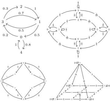
The validation of the proposed algorithm has been per-formed on a set of 9 differentρ-reversible chains, with sizes ranging from 8 to 24 nodes. While testing the method with larger chains would be interesting for evaluating the compu-tational efficiency, it would be very difficult to synthetically produce largeρ-reversible chains. On the other hand, test-ing the method with nonρ-reversible graphs would result in an immediate trivial answer by the algorithm. The first 4 processes are modeled by discrete time Markov chains and are not related to any specific real-world scenario. They are just designed in order to exhibit a valid renaming function and to offer a variable number of states. These synthetic chains, labeled with identifiers from DTMC1 to DTMC4, are presented in Fig. 1. They range from a minimum of 5 states to a maximum of 10 states for the most complex case. In addition to these discrete time chains, we also tested the behavior of the algorithm with 5 continuous time Markov chains, by first transforming them as described in Section 4. These latter chains have been obtained by modeling a practical scenario.
In detail, we show how the proposed algorithm can be applied to a model of a real system. To this end, the al-gorithm is used to verify the ρ-reversibility of the Markov chain underlying the analytical model used for the perfor-mance evaluation of the Fair Allocation Control Window (FACW) protocol [11].
The main idea of FACW is that data traffic in a Wireless Sensor Network (WSN) can be classified into a finite set of M classes K = {c1, c2, . . . , cM}. Each sensor maintains a
control window of sizeN in which the classes of the latest N transmissions (listened or performed) are stored. In the window, at mosthc entries of class c can appear. In case the sensor generates a packet of classcwhen in its window there are already hc entries of classc, the packet is either rescheduled for transmission after a back-off time or simply dropped. Otherwise, in case of generation of a classcpacket when the number ofc-entries in the window is strictly lower thanhc, the packet is sent and the window is updated ac-cording to a FIFO policy. The initialization of the window is arbitrary.
We consider a setK={c1, c2, . . . , cM}ofMdistinct
traf-fic classes and assume that each node maintains a windowW
of sizeNstoring the transmission classes of the most recent sensed data according to a FIFO policy. The state of the window is denoted by~x= (x1, x2, . . . , xN), where xi ∈ K,
and |~x|c = PNi=1δxi=c represents the total number of
oc-currences of classc inW. Data of different traffic classes are generated according to independent Poisson processes
2 3 1 0 4 1 0.3 0.7 0.5 0.5 0.2 0.8 1 3 2 0 1 5 4 6 7 1 2 3 10 1 5 2 5 3 5 2 5 3 5 1 2 1 5 3 10 1 2 1 5 3 10 2 5 3 5 2 5 3 5 1 2 1 5 3 10 0 4 5 3 1 7 6 2 1 2 12 1 1 1 2 1 2 1 2 1 2 1 1 1 2 12 9 4 0 5 3 8 1 7 2 6 5 6 1 12 1 12 1 3 2 3 13 23 23 1 6 1 6 1 1 3 1 3 1 3 1 2 3 1 6 1 6 1 3 2 3 23 1 3
Figure 1: The 4 synthetic discrete time Markov chains used for experimental validation. In the text we will refer to these chains as DTMC1 and DTMC2 for the examples in the first row and DTMC3, DTMC4 for those on the second row. whose ratesλc(j), withc∈ K and 1≤j ≤N, depend on the number of objects j = |~x|c of classc that are present in the window. Clearly, the processX(t) that describes the state ofWis a CTMC. In the window there can be at most hcobjects of classc, withc∈ K. Ifhc=Nthen there is no constraint on the maximum number of objects of the same class in the window. Let~x= (x1, . . . , xN) be the state of
the control window, then the transition rates in the CTMC infinitesimal generator are: for~x6=~x0,
q(~x, ~x0) = (
λc(|~x|c) if~x0= (c, x1, . . . , xN−1) and|~x|c< hc
0 otherwise.
We created a total of 5 different CTMCs based on the FACW model with the parameters showed in Table 3.
Chain N hc |S| Classes Ratesλ
CTMC1 3 3 8 {1,2} {1.0,2.0}
CTMC2 4 3 14 {1,2} {1.0,2.0}
CTMC3 4 4 16 {1,2} {1.0,2.0}
CTMC4 2 2 16 {1,2,3,4} {1.0,2.0,3.0,4.0}
CTMC5 3 2 24 {1,2,3} {1.0,2.0,3.0}
Table 1: Parameters for the FACW model of the generated CTMCs
5.1
Efficiency of the algorithm
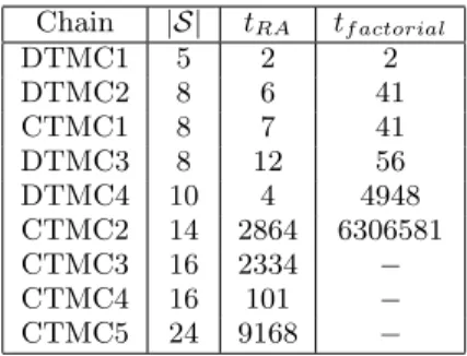
In order to assess the efficiency of the proposed algorithm we compare its execution times with the naive approach. From Table 2 we can notice the improvement in the execu-tion times, the Renaming Algorithm (column tRA) is able to verify theρ-reversibility of the tested chains much faster than the naive approach (column tf actorial). It should be noted that we were not able to complete the computation using the naive approach for all the chains. In fact, with a size of the state space of 16 or more the naive method did not terminate after a whole 24 hours.
Chain |S| tRA tf actorial DTMC1 5 2 2 DTMC2 8 6 41 CTMC1 8 7 41 DTMC3 8 12 56 DTMC4 10 4 4948 CTMC2 14 2864 6306581 CTMC3 16 2334 − CTMC4 16 101 − CTMC5 24 9168 −
Table 2: Execution times in milliseconds
5.2
Suitability of the results
The congruence of the renaming function obtained is easy to verify in practice and the correctness of the verification method has been proven theoretically. Still, we are inter-ested in showing a practical application of the obtained re-naming function and to highlight its suitability with respect to other methods that can be used to obtain the same result. To this end we decided to exploit the renaming map to compute the stationary distribution of tested chains. In fact the notion of ρ-reversibility, as shown in [8], can be used to efficiently compute the vectorπ. We also computed the stationary distribution for the same chains by adopting the rather standard power method simulation (i.e., repeated multiplications).
In Tables 3 and 4 we compare the approximation error of the stationary distribution resulting from the direct compu-tation over the renaming function with the power method after respectively 50 and 100 iterations. In detail, Table 3 shows the results for the discrete time examples and Table 4 reports the results for the continuous time chains. Approx-imations error for the discrete case has been computed as = |πP−π|2
. Differently, we computed the error for the continuous case as = |πQ|2
. It can be observed that, in general, the direct computation through the itera-tive method requires a large number of iterations to obtain a level of accuracy comparable with that of our method.
Chain |S| RA mult50 mult100
DTMC1 5 7.881E−17 3.429E−5 2.299E−8
DTMC2 8 0.0 5.551E−17 0.0
DTMC3 8 0.0 3.065E−11 0.0
DTMC4 10 5.551E−17 6.218E−9 1.582E−15 Table 3: Discrete chains
Chain |S| RA mult50 mult100
CTMC1 8 0.0 0.0 0.0
CTMC2 14 0.0 1.175E−6 1.881E−9
CTMC3 16 0.0 0.0 0.0
CTMC4 16 3.119E−16 2.775E−17 1.387E−17 CTMC5 24 5.846E−17 3.869E−7 1.419E−10
Table 4: Continuous chains
6.
CONCLUSIONS
In this paper we proposed a practical algorithm that al-lows the computation of all the renamings functions for both continuous and discrete time Markov chains. Our algorithm reduces the number of renaming functions that need to be tested by exploiting: properties about the structure of the chain; rules of algebra on the logarithmic function applied to the Kolmogorov’s criterion; and the properties of shortest paths connecting states in the chain.
We compared the execution times of our algorithm with those required by the naive approach showing that the for-mer is much faster than the latter, and that it can obtain solutions where the naive approach cannot. As far as we know our is the first proposal for solving this problem.
As future work we plan to implement other heuristics for polynomially pruning the set of possible renamings and to extensively test them on large systems.
Acknowledgments. Research partially supported by Uni-versity of Udine PRID ENCASE project and by INDAM-GNCS project ”Logica e Automi per il Model-Checking Intervallare”
7.
REFERENCES
[1] S. Balsamo, F. Cavallin, A. Marin, and S. Rossi. Applying reversibility theory for the performance evaluation of reversible computations.In Proc. of ASMTA, 9845 LNCS:45–59, 2016.
[2] S. Balsamo and G. Iazeolla. Aggregation and
disaggregation in queueing networks: The principle of product-form synthesis. InComputer Performance and Reliability, pages 95–109, 1983.
[3] S. Balsamo and A. Marin. Performance engineering with product-form models: efficient solutions and applications. InProc. of ICPE, pages 437–448, 2011. [4] P. G. Harrison. Turning back time in Markovian
process algebra.Theoretical Computer Science, 290(3):1947–1986, 2003.
[5] J. Hillston, A. Marin, S. Rossi, and C. Piazza. Contextual lumpability. InVALUETOOLS, pages 194–203, 2013.
[6] F. Kelly.Reversibility and stochastic networks. Wiley, New York, 1979.
[7] A. Marin and S. Rossi. Autoreversibility: exploiting symmetries in Markov chains. InProc. of MASCOTS, pages 151–160, 2013.
[8] A. Marin and S. Rossi. On discrete time reversibility modulo state renaming and its applications. In
VALUETOOLS, 2014.
[9] A. Marin and S. Rossi. On the relations between lumpability and reversibility. InIn Proc. of MASCOTS, pages 427–432, 2014.
[10] A. Marin and S. Rossi. On the relations between markov chain lumpability and reversibility. InActa Informatica, pages 1–39, 2016.
[11] A. Marin and S. Rossi. Priority-based bandwidth allocation in wireless sensor networks.EAI Endorsed Trans. Wireless Spectrum, 2(10), 2016.
[12] A. Marin and S. Rossi. On the relations between Markov chain lumpability and reversibility.Acta Inf., 54(5):447–485, 2017.
[13] U. Sumita and M. Rieders. Lumpability and time reversibility in the aggregation-disaggregation method for large markov chains.Communications in Statistics: Stochastic Models, 5:63–81, 1989.
[14] P. Whittle.Systems in stochastic equilibrium. John Wiley & Sons Ltd., 1986.