Statistical models and the global temperature record

Statistical_Models_Climate_Change_May_2013_Final - 1 – © Crown copyright 2008

Statistical models

and the global

temperature record

May 2013

Professor Julia Slingo,

Met Office Chief Scientist

1

Executive Summary

This briefing paper has been produced to provide background information relating to analyses undertaken in response to a series of Parliamentary Questions on the use of statistical models to assess the global temperature record, and to address misleading ideas currently appearing in various online discussions.

The global mean warming observed since the late 19th century is far outside the range of observational uncertainty in global temperature datasets, and there is therefore no doubt that the world has warmed. A wide range of observed climate indicators continue to show changes that are consistent with a globally warming world, and our understanding of how the climate system responds to rising greenhouse gas levels.

The analysis of the nature and causes of climate change is based on comprehensive observations of the climate system in combination with theoretical understanding of its physics and general circulation models, themselves based on the fundamental laws of physics. Sophisticated statistics are used to demonstrate the significance of recent changes in the climate system.

Statistical models seek to assess the statistical properties of a specific set of data, in this case the global mean surface temperature timeseries. The models mentioned in the recent Parliamentary Questions are mathematical constructs that are not rooted in the fundamental laws of physics. In comparison with global scientifically based climate models, they are too crude to capture the complexity and non-linearity of the holistic climate system, its internal variability and its physical response to external forcing agents. It should be noted that the Met Office does not rely solely on statistical models in its detection and attribution of climate change.

The Parliamentary Questions requested a statement of the relative likelihood of one statistical model rather than another, emulating the statistical properties of the instrumental record of global average temperature. The models concerned were a linear trend model with first-order autoregressive noise and a driftless third-order autoregressive integrated model. The Met Office has performed this analysis as requested, noting however that the results depend on the starting date of the timeseries, and which of the three global surface temperature datasets is used.

The results show that the linear trend model with first-order autoregressive noise is less likely to emulate the global surface temperature timeseries than the driftless third-order autoregressive integrated model. The relative likelihood values range from 0.001 to 0.32 for the time periods and datasets studied, where a value of 1 equates to equal likelihoods. This provides some evidence against the use of a linear trend model with first-order autoregressive noise for the purpose of emulating the statistical properties of instrumental records of global average temperatures, as would be expected from physical understanding of the climate system.

This is not, however, evidence for the efficacy of the driftless autoregressive integrated model. Similar comparisons between the driftless (trendless) model and two autoregressive integrated models that allow for drift (trend) give likelihood values ranging from 0.45 to 2.58 for the HadCRUT4 dataset. The comparison is therefore inconclusive in terms of selecting the notionally best model. Furthermore, these comparisons do not provide evidence against the existence of a trend in the data.

2

These results have no bearing on our understanding of the climate system or of its response to human influences such as greenhouse gas emissions and so the Met Office does not base its assessment of climate change over the instrumental record on the use of these statistical models.

Nor do the results provide any reason to disregard observational evidence of global warming. In an analysis such as that undertaken here, if the tested models are poorly specified then even the most likely of the tested set of models will be a poor representation of the behaviour of the real climate. In such cases the relative likelihood of the models considered here is of little scientific value.

Setting the context: External forcing agents and indicators of

change

Weather and climate science is founded on observing and understanding our complex and evolving environment. It is therefore an inherent requirement that climate s

available the best possible information on the current state of the climate, and on its historical context. This draws on globally distributed observations and monitoring systems and networks. This is also dependent on robust data processing

amounts of data, properly taking into account observational uncertainty resulting from both measurement limitations and sampling. Only through taking due diligence and applying rigorous, unbiased, scientific assessment, can

picture on the state, trends and variability of the climate system’s many variables and phenomena. This provides the basis on which the science can advance and provide the evidence base and advice required by d

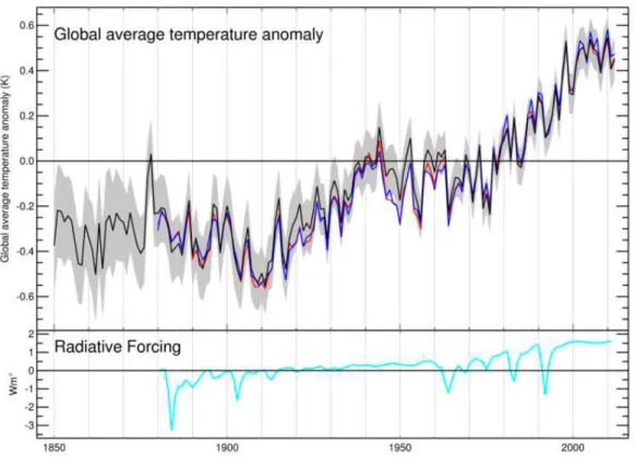
Over the period of the instrumental record, dating back to the 1850s, global average combined land-sea temperature has increased by around 0.8 °C.

independent global average temperature series, shown in F decade has been the warmest on record.

so has the radiative forcing of the planet as a result of increased greenhouse gas concentrations.

Figure 1: (a) Global mean surface tem

et al, 2012)2, red MLOST Based on Smith et al. (2008) Radiative forcing, Wm-2 , GISS-

1

Met Office, ‘Our changing climate

2

Morice, C. P., J. J. Kennedy, N. A. Rayner, and P. D. Jones (2012), Quantifying uncertainties in global and regional temperature change using an ensemble of observational estimates: The HadCRUT4 dataset, J. Geophys. Res., 117, D08101, doi:10.1029/

3

Setting the context: External forcing agents and indicators of

Weather and climate science is founded on observing and understanding our complex and evolving environment. It is therefore an inherent requirement that climate s

available the best possible information on the current state of the climate, and on its historical globally distributed observations and monitoring systems and networks. This is also dependent on robust data processing and analysis to synthesise vast amounts of data, properly taking into account observational uncertainty resulting from both measurement limitations and sampling. Only through taking due diligence and applying rigorous, unbiased, scientific assessment, can climate scientists provide the most complete picture on the state, trends and variability of the climate system’s many variables and phenomena. This provides the basis on which the science can advance and provide the

nce base and advice required by decision-makers.

Over the period of the instrumental record, dating back to the 1850s, global average sea temperature has increased by around 0.8 °C.1

e temperature series, shown in Figure 1, agree that the last decade has been the warmest on record. At the same time as the temperatures have risen, so has the radiative forcing of the planet as a result of increased greenhouse gas

(a) Global mean surface temperature 1850 – 2012 (K) ,Black-HadCRUT4 Based on Morice , red MLOST Based on Smith et al. (2008)3,GISTEMP Based on Hansen et al. (2010)

http://data.giss.nasa.gov.

Our changing climate: Trends, extremes, attribution and projections’, 2012.

Morice, C. P., J. J. Kennedy, N. A. Rayner, and P. D. Jones (2012), Quantifying uncertainties in global and regional temperature change using an ensemble of observational estimates: The HadCRUT4 dataset, J. Geophys. Res., 117, D08101, doi:10.1029/2011JD017187

Setting the context: External forcing agents and indicators of

Weather and climate science is founded on observing and understanding our complex and evolving environment. It is therefore an inherent requirement that climate scientists have available the best possible information on the current state of the climate, and on its historical globally distributed observations and monitoring systems and and analysis to synthesise vast amounts of data, properly taking into account observational uncertainty resulting from both measurement limitations and sampling. Only through taking due diligence and applying climate scientists provide the most complete picture on the state, trends and variability of the climate system’s many variables and phenomena. This provides the basis on which the science can advance and provide the Over the period of the instrumental record, dating back to the 1850s, global average

1 _{All three of the}

igure 1, agree that the last At the same time as the temperatures have risen, so has the radiative forcing of the planet as a result of increased greenhouse gas

HadCRUT4 Based on Morice ,GISTEMP Based on Hansen et al. (2010)4 (b)

’, 2012.

Morice, C. P., J. J. Kennedy, N. A. Rayner, and P. D. Jones (2012), Quantifying uncertainties in global and regional temperature change using an ensemble of observational estimates: The

4

Figure 2: The top panel shows the observed global mean air surface temperature anomaly from HadCRUT3 (grey line) and the best multivariate fits using the methods of Lean and Rind [2009] (blue line), Lockwood [2008] (red line), Folland et al. [2011] (green line) and Kaufmann et al. [2011] (orange line). The remaining panels show the individual temperature contributions to the top panel fits from ENSO (second panel), volcanoes (third panel), solar irradiance (fourth panel), anthropogenic contribution (fifth panel) and other factors (sixth panel). Other factors shown in the sixth panel include the AMO for Folland et al. [2011], and minor annual, semi-annual and 17.5 years cycle identified by Kopp and Lean, [2011] in the residuals of Lean and Rind [2009]’s model. From Imbers et al (2013)5.

3

Smith, T. M., R. Reynolds, T.C. Peterson and J. Lawrimore (2008), Improvements to NOAA's Historical Merged Land-Ocean Surface Temperature Analysis (1880-2006), Journal of Climate, 21, 2283-2293

4

Hansen, J., R. Ruedy, M. Sato, and K. Lo (2010), Global surface temperature change, Rev.

Geophys., 48, RG4004, doi:10.1029/2010RG000345

5

Imbers J., A. Lopez, C. Huntingford, and M. R. Allen (2013), Testing the robustness of the anthropogenic climate change detection statements using different empirical models, J. Geophys. Res. Atmos., 118, 3192–3199, doi:10.1002/jgrd.50296.

5

Although greenhouse gas concentrations, especially carbon dioxide, have risen steadily, the climate we experience is affected by a number of other factors. These factors can be internal to the climate system (e.g. interactions occurring between the atmosphere and ocean, often referred to as natural internal variability) or external (e.g. occurring outside of the climate system, such as a change in the amount of energy being output by the Sun).

Figure 2 shows a range of the most important of these internal and external factors and estimates of the contributions they have made to the observed global temperature rise since the late 19th century.

The Atlantic Multi-decadal Oscillation is a mode of natural variability occurring in the North Atlantic Ocean that is defined by sea surface temperature patterns. The El Nino Southern Oscillation is an interaction between the atmosphere and the Pacific Ocean. The Oscillation has two phases: El Nino, where there is warming of the East Pacific Ocean and La Nina, where there is cooling. Both of these modes of natural variability have a strong influence on global temperatures and regional climates around the world.

Volcanoes, the Sun and greenhouses gases are external forcings on the climate system. Powerful volcanoes can temporarily reduce the global temperature, by emission of sulphate aerosols into the stratosphere which act to reflect incoming solar radiation. Changes in the activity of the Sun can contribute positively or negatively to global temperature change, while greenhouse gases drive rising temperatures.

The climate is a physical system governed by physical laws. It is only through observing and understanding the climate system and the influence and interaction between all the factors that can affect it, that we can detect changes in the system and attribute them to their causes. To negate the physical nature of the climate system in any study on climate variability or change means the study is neglecting the governance of physical law.

Brohan P, J.J. Kennedy, I. Harris, S.F.B. Tett and P.D. Jones. (2006), Uncertainty estimates in regional and global observed temperature changes: a new dataset from 1850. J. Geophys. Res. 111: D12106, doi:10.1029/2005JD006548.

Lean, J., and D. H. Rind (2009), How will earths surface temperature change in future decades?,

Geophysical Research Letters, 36, L15,708.

Lockwood, M. (2008), Recent changes in solar outputs and the global mean surface temperature. iii. analysis of contributions to global mean air surface temperature rise, Proceedings of the Royal Society

A: Mathematical, Physical and Engineering Science, 464 (2094), 1387–1404

Folland, C., A. Colman, J. Kennedy, J. Knight, D. Parker, P. Stott, D. Smith, and O. Boucher (2011), High predictive skill of global surface temperature a year ahead, in AGU Fall Meeting Abstracts, vol. 1, p. 01.

Kaufmann, R., H. Kauppi, M. Mann, and J. Stock (2011), Reconciling anthropogenic climate change with observed temperature 1998–2008, Proceedings of the National Academy of Sciences, 108 (29), 11,790.

Kopp, G., and J. Lean (2011), A new, lower value of total solar irradiance: Evidence and climate significance, Geophys. Res. Lett., 38, L01,706.

6

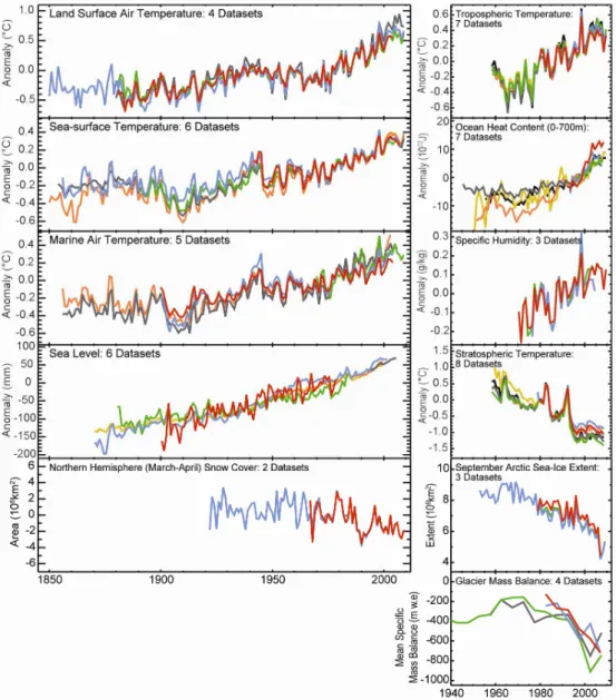
The global mean temperature at the surface of the Earth, shown in Figure 1, is often used as the primary indicator of climate change, and often as the only indicator in many discussions. National and international negotiations on climate change tend to focus on ways of limiting global mean surface temperature rise to no more than 2°C, this being a goal of the United Nations Framework Convention on Climate Change. However, in addition to surface air temperature, there are many other key indicators that can help to gauge the state of the climate, drawn from observations of the atmosphere, the oceans, and the cryosphere (snow and ice). The compilation of the eleven indicators shown in Figure 3 has drawn on the work of over 100 scientists from more than 20 institutions, and provides a more comprehensive assessment of the state of the climate than global mean surface temperature alone6.

Figure 3: Time series from a range of indicators that would be expected to correlate strongly with the

surface record. Note that stratospheric cooling is an expected consequence of greenhouse gas increases.6

6

Kennedy J.J., P.W. Thorne, T.C. Peterson, R.A. Ruedy, P.A. Stott, D.E. Parker, S.A. Good , H.A. Titchner, and K.M. Willett, 2010: How do we know the world has warmed? [in .State of the Climate in 2009.]. Bull. Amer. Meteor. Soc., 91 (6), S26-S27.

7

The changes in these indicators continue to show changes that are consistent with a globally warming world, and our understanding of how the climate system responds to rising greenhouse gas levels. It is our understanding of the changes in the holistic climate system and the contribution of the various external forcing agents to those changes that lie at the heart of statements around the detection and attribution of global mean surface temperature rise.

8

Statistical Models of Instrumental Records of Global Surface

Temperature Change

Physical understanding of the climate tells us that in the absence of external forcings, global temperatures should vary around a climatological average temperature. Temperatures may exhibit long-term persistence in these excursions away from the climatological average as a result of internal variability in the system.

The climate is also influenced by external forcings such as changes in concentrations of CO2

and other greenhouse gases, volcanic and anthropogenic aerosols, ozone depletion, and changes in incoming solar radiation. These factors will also result in long-term persistence in global temperature change, but they can potentially be accounted for in statistical analysis, since we have observations of these quantities.

A well-posed statistical model of global temperature evolution should be able to model changes in the mean state of the system (if any such change is identified), as well as modelling persistence in departures from the mean state. A well-posed statistical model should also take into account known external influences on the studied series. Without doing so, the effects of these influences are otherwise treated as random processes rather than known quantities, reducing the power of the chosen model to make inferences about the real world.

The following discussion relates to a series of Parliamentary Questions7 debating which of two statistical models is the most appropriate for modelling the evolution of global mean surface temperature. From a scientific perspective, knowing both the complexity of the physical climate system and of the external forcing agents in space and time (Figures 2 and 3), it is debatable whether one or another of these statistical models has the capability to capture those complexities; both models are far too naive in their construction to capture the complexity of the real world, and neither account for external forcings.

Thus, the Met Office does not use one of these statistical models to assess global temperature change in relation to natural variability. In fact, work undertaken at the Met Office on the detection of climate change in observational data is predominantly based on the application of formal detection and attribution methods. These methods combine observational evidence with physical knowledge of the climate (in the form of general circulation models) and its response to external forcing agents, and have a solid foundation in statistics. These methods allow physical knowledge to be taken into account when assessing a changing climate and are discussed at length in Chapter 9 of the Contribution of Working Group I to IPCC AR48.

7

(WA 110), 5 February (WA 31-2), 21 March (WA 170-1), 23 April (WA 359)

8

IPCC, (2007), Climate Change 2007: The Physical Science Basis. Contribution of Working Group I to the Fourth Assessment Report of the Intergovernmental Panel on Climate Change [Solomon, S., D. Qin, M. Manning, Z. Chen, M. Marquis, K.B. Averyt, M.Tignor and H.L. Miller (eds.)]. Cambridge University Press, Cambridge, United Kingdom and New York, NY, USA

9 The two statistical models in question

A statistical model is defined as a mathematical description of a system or process in terms of random variables, typically taking the form of a simplified mathematical representation of a complex system. In the context of this document a statistical model can be thought of as a simplified mathematical framework designed to generate time series with similar statistical properties to instrumental records of global average temperature change.

It is impossible to define a ‘true’ statistical model of the real world because we do not know all the detail of the real world. At best, statistical models can only be relatively crude emulators of the real climate system because of the complexity and huge number of degrees of freedom of that system. Since there is no ‘true’ model, researchers in this field may look at the relative likelihood of one statistical model versus another emulating the statistical properties of the data under consideration. Of course, deciding what might be a reasonable formulation for the statistical model in the first place, should require an understanding of the attributes of the system under consideration, such as spatial and temporal scales of natural climate variability and the response of the climate system to external forcings.

In the following analysis we therefore consider the relative likelihood of one type of statistical model providing a better emulation of the statistical properties of the global surface temperature record than another type, as requested in the Parliamentary Questions.

Linear trend with first order autoregressive noise – This model expresses the evolution of the average state of the quantity of interest, in this case recorded global annual surface temperature anomalies (i.e. departures from a long-term average – see Figure 1), as a linear change over time. Departures from the linear trend are assumed to be random (i.e. represented as random noise), although there is a degree of dependence assumed between the departure for a given year and that of the previous year.

The linear trend with first order autoregressive noise model applied to global temperature series, represents changes in the mean state of the climate as a long term linear change. While this is a convenient simple mathematical description of a changing climate, its usefulness for emulating the behaviour of the global mean surface temperature is limited because known forcings on the climate (see Figure 2) are unlikely to result in a linear change in average temperatures. A further issue is that, should the linear change be considered to represent the result of anthropogenic forcing, the most appropriate choice of starting year for the linear change is unclear.

First order autoregressive noise models only allow for short term variability in the climate and do not model long term persistence in global average temperatures that may result from either internal variability (for example arising from low frequency large scale climatological patterns such as the Atlantic Multidecadal Oscillation) or external forcings (such as changes in solar forcing).

Uncertainty in the most appropriate choice of starting year for a linear trend and the lack of capability of a first order autoregressive process to model long term persistence in the climate, results in a high sensitivity of the fitted model parameters (i.e. estimates of the trend, the mean state and autoregressive coefficient) to the time period studied.

This model is the one assumed, incorrectly, to be used by the Met Office to assess global temperature change in relation to natural variability.

10

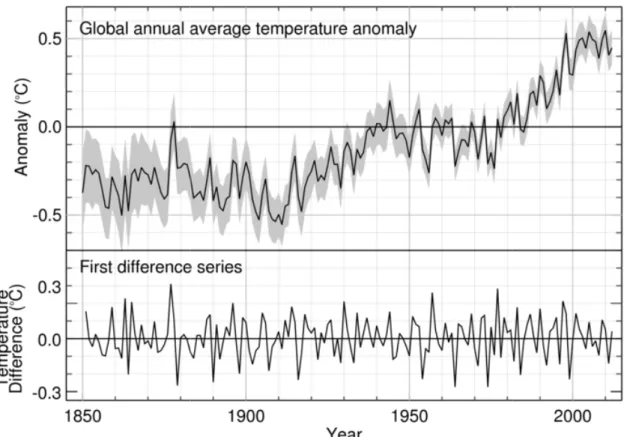
Autoregressive integrated model – Autoregressive integrated models assume that the change in the quantity of interest from one year to the next can be described as a form of random walk process. For an autoregressive integrated process used to model the evolution of global annual average surface temperature changes, the size and direction of the random walk steps are dependent on the random walk in previous years, with persistence in the magnitude and direction of the random walk steps. This is effectively equivalent to fitting an autoregressive process to a first difference series (temperature change from year to year) rather than directly fitting an autoregressive process to a global average temperature anomaly series (Figure 4).

Time series generated from an autoregressive integrated process are not constrained to return to an average state but are free to slowly progress away from an initial value. An autoregressive integrated model allows long term persistence in the climate, but the random walk process is not constrained to vary around a climatological average value, a property that is not consistent with the notion of a climate that is in a steady state.

For a third order autoregressive model, the random walk step for a given year is dependent on the size and direction of the modelled random walk steps in the previous three years. In the context of application of this model to global temperature change, this model could be taken to describe longer-term random variation in the climate. An integrated model with drift can be considered to be equivalent to a random walk process superimposed on a linear trend. An integrated model without drift is equivalent to a random walk without a linear trend. The driftless third order autoregressive integrated model does not include a drift component and so can be considered to be a form of random walk model that does not allow for a linear trend.

Additional models studied in the peer reviewed scientific literature – Further studies on statistical methods to describe the development of global temperatures over the instrumental period continue to be published in well regarded peer reviewed scientific journals9. These studies consider an additional class of models, known as autoregressive fractionally integrated moving average models.

These models exhibit two desirable properties for modelling global temperatures: they model series that are constrained to vary around a climatological average and they allow representation of long-term persistence in departures in that average. However, there is still debate on how well these models represent the observed temperature records and hence on the utility of these models in statistical analysis of the global temperature evolution.

9

Cohn, T. A. and H. F. Lins, 2005, Nature's style: Naturally trendy, Geophys. Res. Lett., 32, L23402, doi:10.1029/2005GL024476.

Koutsoyiannis, D., Montanari, A. (2007). Statistical analysis of hydroclimatic time series: Uncertainty and insights, Water Resour. Res., Vol. 43, W05429, doi:10.1029/2006WR005592

Rybski, D., A. Bunde, S. Havlin, and H. von Storch (2006), Long-term persistence in climate and the detection problem, Geophys. Res. Lett., 33, L06718, doi:10.1029/2005GL025591

Zorita, E., T. F. Stocker, and H. von Storch (2008), How unusual is the recent series of warm years?, Geophys. Res. Lett., 35, L24706, doi:10.1029/2008GL036228

Figure 4: Top: The HadCRUT4 global te

year differences in the global temperature record.

models this first-difference series as a third order autoregressive process

Statistical Model Comparison

The Parliamentary Questions ask for a comparison between the linear trend with first autoregressive noise model and a driftless third

terms of their relative likelihood of emulating a

instrumental records of global average temperature change. Both of the models under consideration

random process without explicitly considering ex

influences can be taken into account in statistical modelling by treating them as known external factors affecting global average temperature.

discussed here the effects of these

so must instead be considered to be part of the random noise component of the statistical model. Treating known forcings as random noise in this way limits the facility of the models in question to detect changes in the mean state of the climate.

The models also assume that the statistical properties of the global temperature series are constant, i.e. they do not change with time. They take no account of the estimated uncertainty in the observed global averag

record.

11

Top: The HadCRUT4 global temperature anomaly series. Bottom: Time

year differences in the global temperature record. The driftless third order autoregressive process difference series as a third order autoregressive process.

Comparison

The Parliamentary Questions ask for a comparison between the linear trend with first autoregressive noise model and a driftless third-order autoregressive integrated model, in terms of their relative likelihood of emulating a time series with similar statistical properties to instrumental records of global average temperature change.

under consideration treat the evolution of global temperatures as a random process without explicitly considering external forcings on the system.

influences can be taken into account in statistical modelling by treating them as known external factors affecting global average temperature. However, in both

the effects of these observed variables are not explicitly accounted for so must instead be considered to be part of the random noise component of the statistical model. Treating known forcings as random noise in this way limits the facility of the models

anges in the mean state of the climate.

The models also assume that the statistical properties of the global temperature series are i.e. they do not change with time. They take no account of the estimated uncertainty in the observed global average temperature series, which is larger in the early mperature anomaly series. Bottom: Time series of

year-to-The driftless third order autoregressive process

The Parliamentary Questions ask for a comparison between the linear trend with first-order autoregressive integrated model, in ith similar statistical properties to treat the evolution of global temperatures as a ternal forcings on the system. External influences can be taken into account in statistical modelling by treating them as known However, in both the models variables are not explicitly accounted for, and so must instead be considered to be part of the random noise component of the statistical model. Treating known forcings as random noise in this way limits the facility of the models The models also assume that the statistical properties of the global temperature series are i.e. they do not change with time. They take no account of the estimated which is larger in the early

12

When comparing statistical models in terms of likelihoods it is common to undertake the comparison using a metric that penalises complex models, so as to prevent over-fitting of the model to the data by selecting an arbitrarily complex model. One such metric is the corrected Akaike Information Criterion (AICc), which is used for model comparison in this study.

Comparison of the two statistical models considered in the Parliamentary Questions is complicated by the fact that the two models are not nested, i.e. they have different mathematical forms. One operates on the series in question, i.e. a series of global annual average temperature anomalies, whereas the other operates on a difference series, i.e. a series constructed from the difference in temperature from year to year (see Figure 4). Indeed, it is often the case that it is not possible to use the corrected Akaike Information Criterion to compare two statistical models that are not nested. This complication means that it is not simple to assess the relative likelihood of these two statistical models using standard model comparison techniques.

To allow model comparison here we adopt the method of Zheng and Basher (1999)10 to express the two models within the same mathematical framework and so allow comparison of statistical models that differ in this regard. The studied models are then fitted to a global temperature time series and their relative likelihoods of producing a time-series identical to the instrumental record of global average temperature change are computed using the corrected Akaike Information Criterion (AICc) for each model. This criterion is a measure of the likelihood of the statistical model that penalises model complexity.

As the results are dependent on the length of the time series and the dataset used (neither of which have been defined in the Parliamentary Questions), we perform the analysis across a range of time-series length and datasets. We have done this to test how robust the results are to the choice of period studied.

Note we do not take start years later than 1900 in order not to penalise the ARIMA models, which perform worse than the linear model with first order auto-regressive noise when fitted to time scales of the order of a few decades, eg from 1970 to present. In this study it is not appropriate to fit the models to periods of a few decades or less as such an application would not allow a fitted model to describe known low frequency variability in the climate of the order of multi-decadal time scales. However, in other applications in which natural variability is considered to be part of the signal of interest, rather than noise, application to shorter periods may be appropriate.

Table 1 shows the likelihood of a small range of models being able to emulate the statistical properties of the instrumental record of global average temperature change, compared to the driftless third-order autoregressive model. The numerical results are therefore relative likelihoods. This means that a value of 1.0 would indicate that the listed model and the driftless third-order autoregressive integrated model are equally likely to emulate the global annual average surface temperature change. A value of 0.5 would indicate that the listed model is half as likely as the driftless third-order autoregressive model; likewise a value of 2

10

Zheng, X and R.E. Basher, (1999). Structural Time Series Models and Trend Detection in Global and Regional Temperature Series. J. Climate, 12, 2347–2358.

13

means that the listed model is twice as likely as the driftless third-order autoregressive model.

The results in the first column are the comparison requested through the Parliamentary Questions. The second and third column shows the results of comparisons of the driftless third-order autoregressive model with two models that allow drift (i.e. a trend). These have been chosen for illustrative purposes to show that other statistical models exist which could be applied to the question, and that the requested comparison cannot be taken as proof of the absence of a trend in the time series.

Start Year

Linear model with first order auto-regressive noise

Third order autoregressive integrated model with drift (ARIMA(3,1,0)

First order autoregressive

integrated moving average model with drift (ARIMA(1,1,1)

1850 0.001 0.71 1.23 1860 0.005 0.83 2.58 1870 0.006 0.72 0.62 1880 0.02 0.73 0.77 1890 0.06 1.46 0.48 1900 0.08 1.07 0.45

Table 1 - The relative likelihood of three statistical models in comparison to the proposed driftless ARIMA(3,1,0) model when fitted to HadCRUT4 global annual average temperature anomalies over a period from the start year indicated to 2012. The notation ARIMA (p,d,q) denotes: p the number of autoregressive parameters, d the level of differencing and q the number of moving average parameters of an autoregressive integrated moving average model.

As noted, the results are dependent on time series length and dataset. For example, considering the period from 1900 to 2012, the relative likelihood of the two models being able to generate a time series with similar properties to the instrumental records of global average temperature change using HadCRUT4 is 0.08, whereas the relative likelihood over the same period using NOAA’s dataset is 0.32, and the same calculation using NASA’s dataset indicates a relative likelihood of 0.10.

The likelihood that the linear trend model with first-order autoregressive noise represents better the evolution of global annual average surface temperature anomalies than the driftless third-order auto regressive integrated model is small for all periods considered in Table 1. This provides some evidence against the use of a linear trend model with first-order autoregressive noise to emulate the observed global temperature record, as we would expect from our physical understanding of the climate system.

This is not however evidence for the efficacy of the driftless autoregressive integrated model. As the second and third columns in Table 1 show, comparisons between the driftless (trendless) model and the two models that allow for drift (trend) are inconclusive in terms of selecting the notionally best model. Notably, the relative likelihoods of the two models that do allow for drift (trend) versus the driftless model proposed in the Parliamentary Questions, do not provide evidence against the existence of a trend in the data.

Furthermore, it should be noted that the two models referred to in the Parliamentary Questions are far from an exhaustive list of available statistical models that could be tested. Studies of statistical modelling of global temperatures in the peer reviewed scientific literature are not limited to the comparison of two models in isolation, but instead compare a wide

14

range of models in relation to one another. It is valid to expect that, if such a study was performed, other statistical models may exist that perform better than the driftless third-order autoregressive integrated model in such a comparison.

Statistical model comparisons, such as that described here, do not allow the identification of a ‘true’ model, only the computation of the relative likelihood of the models considered. Additionally, these statistical models do not take into account the physics of the climate or any of the known external influences that affect global temperatures. In an analysis such as that undertaken here, if all the tested models are poorly specified then even the most likely of the tested set of models will be a poor representation of the behaviour of the real climate. In such cases the relative likelihood of the models considered is of little scientific value.

15

Conclusions

This briefing paper has been produced in response to a series of Parliamentary Questions on the use of statistical models to interrogate the global temperature record. As the Met Office makes its assessments of global climate change on a wider evidence base and performs detailed detection and attribution studies based firmly in the physics of the climate system, the comparisons in this paper have no bearing on Met Office statements on climate change. The importance of observing the climate and of understanding and modelling the climate system with numerical climate models is vital to the performance of detection and attribution studies.

Our calculations of whether a linear trend with first order autoregressive noise model is more likely to emulate the global temperature timeseries than the driftless third order autoregressive integrated model, show a range of relative likelihood values from 0.001 to 0.32 depending on which dataset is used (HadCRUT4, NASA, NOAA) and the starting date of the timeseries (1850-1900). This means that the driftless third order autoregressive model is more likely to represent the timeseries with these starting dates than the linear trend model.

However, considering the complex physical nature of the climate system, there is no scientific reason to have expected that a linear model with first order autoregressive noise would be a good emulator of recorded global temperatures, as the ‘residuals’ from a linear trend have varying timescales of persistence related to (i) the timescale of the external forcing and the response of the climate system to it and (ii) the inherent timescales of natural climate variability associated with the dynamic adjustment of the oceans/atmosphere coupled system.

The likelihood that the third order autoregressive integrated model with drift (i.e. with trend) will emulate the global temperature series as effectively as the driftless model ranges from 0.71 to 1.46, dependent on time period studied for HadCRUT4. This comparison of the driftless model with those that include drift shows that, even though the driftless model produces a better emulation of the global temperature series than the linear model with first order autoregressive noise, the results cannot be taken as proof against the presence of a trend in the global temperature data. Other models that do allow for a trend perform as well as the proposed driftless autoregressive integrated model

As previously stated, the Met Office’s assessment of global climate change is not based on modelling the evolution of global surface temperature as a linear trend with first-order autoregressive noise. Studies of statistical modelling using a wide range of models continue to be published in the peer-reviewed literature and we continue to take this work, along with other information, into consideration when making assessments of climate change.

Acknowledgement is given to Dr. Colin Morice, Dr. Doug McNeal, Dr. Peter Stott, Dr. Nick Rayner and Dr. John Kennedy, all from the Met Office, for their time and expertise in helping to prepare this paper.