Behavioural Macro-Financial Cycles
Alfred Fitzgerald Lake
Faculty of Economics and Girton College University of Cambridge
This thesis is submitted for the degree of Doctor of Philosophy
January 2020
Declaration
This thesis is the result of my own work and includes nothing which is the outcome of work done in collaboration except as declared in the Preface and specified in the text. I certify that Chapter 2 was co-authored with Dr Laurent Maurin and that I contributed over 50% of the work.
This thesis is not substantially the same as any that I have submitted, or is being concurrently submitted, for a degree or diploma or other qualification at the University of Cambridge or any other University or similar institution except as declared in the Preface and specified in the text. I further state that no substantial part of my thesis has already been submitted, or, is being concurrently submitted for any such degree, diploma or other qualification at the University of Cambridge or any other University or similar institution except as declared in the Preface and specified in the text.
It does not exceed the prescribed word limit of 60,000 words from the Economics Degree Committee.
The copyright of this thesis rests with the author. Quotation from it is permitted, provided that full acknowledgement is made.
Abstract of Behavioural
Macro-Financial Cycles
Alfred Fitzgerald Lake
In the first chapter I study the optimal inflation expectations that it is possible for agents to estimate and the difference between these and rational expectations. It is typically not feasible for an agent with a macroeconomic sample of realistic length to estimate a conditionally unbiased predictor of future variables, such as rational expectations. It is also often not optimal, in terms of forecast error, to minimise the conditional biases imposed, as using statistically simple expectations will often reduce forecast variance sufficiently to outweigh forecast bias. I therefore introduce optimal feasible expectations, the expectations that are predicted to minimise the relevant measure of forecast error out of the set of expectations that agents can esti-mate, as a realistic alternative to infeasible rational expectations. I then empirically estimate the optimal conditional biases when forecasting US inflation using a factor weighted ridge approach. I find it is optimal to impose large conditional biases: one should essentially only use information on past changes in price indices, despite several other variables and factors having economically and statistically significant associations with future inflation. I then compare these to the conditional biases in US household forecast surveys. I find that many of the conditional biases are sim-ilar, although households also make errors that reduce their forecast performance compared to feasible empirical alternatives. Therefore a combination of optimal fea-sible expectations and behavioural errors appear to explain US household inflation forecasts.
In the second chapter I study whether increases in asset price convergence and the quantity of cross-border asset holdings, common measures of financial integra-tion, imply high quality changes in financial integraintegra-tion, i.e. changes that are likely to produce the largest net economic benefits. I use a new methodology based on a Bayesian FAVAR to overcome the econometrically challenging setting and test three aspects of the quality of changes in financial integration measures. I apply this methodology to the EU in the 21st century and find that there is a common factor that drives a wide range of price and quantity integration measures. However the changes in financial integration are primarily cyclical, as long-term cyclicality strongly outweighs deterministic and stochastic trends, and dependent on macroe-conomic conditions, as virtually all sign identified emacroe-conomic shocks cause large cor-responding effects on financial integration. This suggests that increases in financial integration have not been high quality: they actually appear most closely related to cyclical changes in the underlying risks of European assets and aversion to these risks.
In the third chapter I introduce a new test of whether house prices are always equal to their fundamental value, adjusted to account for contractual rigidities and search frictions, based on the speed of their reaction to monetary shocks. I justify this test with two conceptual frameworks and references to existing empirical work on the transmission mechanisms of monetary policy. I then apply this test to house prices in the US using narrative monetary shocks in a local projections approach. I find that real house prices do not react to monetary shocks when contractual rigidities stop binding, however they have economically and statistically significant reactions at horizons over a year. This result is inconsistent with house prices always being equal to their fundamental value, but is consistent with agents either not fully observing monetary shocks or not incorporating these shocks into their expectations rationally. I also use a sign decomposition based on the conceptual frameworks to identify the relative importance of proximal drivers of house price cycles: I find that consumption demand is the most important driver but asset demand is also relatively important. Therefore housing cycles are likely to arise from the partially behavioural reactions to changes in housing demand.
Acknowledgements
Firstly, I want to thank Sean Holly for supervising me. I am grateful to him for his advice and for giving me the intellectual freedom to conduct applied economic research in my own way, despite being in a department that mainly focuses on abstract theory. I also want to thank my co-author Laurent Maurin for his advice and work, which was central to the paper which became the second chapter of this PhD, and Coen Teulings, my advisor and MPhil supervisor, for all his early advice. There are many others, both in Cambridge and outside, to whom I am also grateful to for useful economic discussions. This includes members of the Cambridge faculty, my fellow Cambridge PhD students, my colleagues in Luxembourg and those who taught me economics before my PhD.
I must also express my gratitude to the Cambridge Trust and Girton College, for fully funding me during my time in Cambridge, and to the European Investment Bank for offering me a paid research placement with them in Luxembourg.
Producing this PhD has been challenging at times and the people around me have been hugely supportive. I am lucky to have had friends in the department and the university squash team in Cambridge, as well as in my department in Luxembourg, that made my days more enjoyable. I am also grateful for the great friends I made in Wolfson Court and for my oldest friends back in North London: the three years would not have been the same without them. I want to thank El so much for her love, support and all night trips to Luxembourg: they mean so much to me. Finally I would like to thank my family, in particular my parents. They have been an invaluable source of support and advice all my life and I would not have got to this point without them.
Contents
Thesis introduction 1
1 Optimal feasible expectations in our uncertain economy 13
1.1 Introduction . . . 13
1.2 Conceptual and econometric setup . . . 21
1.3 Macroeconomic data and factors . . . 30
1.4 Conditional biases in optimal feasible inflation expectations . . . 37
1.5 Conditional biases in household inflation forecasts . . . 44
1.6 Conclusion . . . 47
2 Asset price convergence, international asset holdings and the qual-ity of financial integration 51 2.1 Introduction . . . 51
2.2 Econometric methodology . . . 57
2.3 Dataset and estimated financial integration factor . . . 62
2.4 The quality of EU financial integration . . . 66
2.5 Conclusion . . . 72
3 Behavioural finance at home: house price cycles in the USA 74 3.1 Introduction . . . 74
3.2 Testing whether house prices are consistent with fundamentals using monetary shocks . . . 80
3.3 Conducting the test with narrative monetary shock data . . . 87
3.4 New stylised facts on the drivers of housing cycles . . . 93
A Supplement: Behavioural financial cycles as the cause of perpetual
business cycles 104
B Appendix of ‘Optimal feasible expectations in our uncertain
econ-omy’ 114
B.1 Variables used to construct factors . . . 114
B.2 Training set size robustness . . . 118
B.3 Forecast performance measure robustness . . . 122
C Appendix of ‘Asset price convergence, international asset holdings and the quality of financial integration’ 124 C.1 Gibbs sampler . . . 124
C.2 Signed impulse response functions . . . 126
C.3 Convergence robustness . . . 130
C.4 Prior robustness . . . 132
C.5 Extended dataset . . . 136
D Appendix of ‘Behavioural finance at home: house price cycles in the USA’ 138 D.1 Conceptual frameworks . . . 138
D.2 Cycle periodicity robustness . . . 147
D.3 Housing data source robustness . . . 153
Thesis introduction
This thesis studies behavioural macro-financial cycles. Financial cycles and their links to the macroeconomy are an important topic, as information on financial cy-cles can help to detect financial crises in real time (Borio, 2014) and the downturns of financial cycles are associated with serious recessions (Claessens et al., 2012). A behavioural approach to this topic is needed, as it is not appropriate to believe that all agents make financial decisions by maximising utility functions with rational expectations when most individuals cannot correctly answer basic questions on eco-nomic and financial literacy (Lusardi and Mitchell, 2014). This thesis is primarily made up of three self-contained chapters, each of which analyses topics which are related to macro-financial cycles and either explicitly analyses behavioural insights or suggests them as a potential underlying cause of the results. The three main chapters are followed by four appendices and a bibliography.
The first chapter is titled ‘Optimal feasible expectations in our uncertain econ-omy’. In this chapter I analyse the optimal macroeconomic expectations that agents could feasibly estimate and any differences between these optimal feasible expecta-tions and their actual expectaexpecta-tions. It particularly focuses on inflation expectaexpecta-tions due to their importance in macroeconomics.
There is a large macroeconomic learning literature, surveyed in Evans and Honkapo-hja (2012), that models how agents estimate inflation expectations. Papers in this survey often implicitly assume that agents have access to extremely large quantities of relevant data. In this case using rational expectations given the data available to agents is feasible and, since rational expectations are the true conditional expec-tation (Sheffrin, 1996), optimal in terms of minimising measures of forecast error. Some papers in this literature acknowledge that in reality structural change over
time means that limited samples are available (Orphanides and Williams, 2007), however they usually use models with so few variables that it is still possible to estimate conditionally unbiased estimators. The first contribution of this chapter is to discuss clearly why estimating conditionally unbiased expectations, such as rational expectations, will usually be impossible in reality. It is usually statistically impossible as there are a a far greater number of potentially relevant macroeconomic variables than there are relevant time series observations of each of these variables. This seems very unlikely to change in the foreseeable future, as the rise of big data makes even more variables available and the economy undergoes structural change as a result of the response to Covid-19. It also clearly discusses why it may often not be optimal to try and limit the degree of conditional biases imposed. This is because it may often be worth shrinking expectations towards those that are sta-tistically simpler to reduce the conditional variance of forecasts even if it imposes greater conditional biases in forecasts. This insight is at the heart of many modern machine learning approaches to forecasting, such as those in Medeiros et al. (2020). It therefore introduces optimal feasible expectations, namely the expectations that are predicted to minimise the relevant measure of forecast error out of the set of expectations that agents can estimate.
The econometric optimal inflation forecasting literature finds that very simple inflation forecasts perform best in forecasting horse races (Faust and Wright, 2013). Therefore the optimal forecasts suggested by this literature do not incorporate any associations between the vast majority of macroeconomic variables and future infla-tion. However this literature does not typically try to estimate the true associations between macroeconomic predictors and future inflation and so does not examine the conditional biases in optimal econometric inflation forecasts. The second con-tribution of this chapter is to estimate both the true associations between a set of macroeconomic variables and future inflation and the associations that it is optimal to use in forecasting. The difference between the two is the conditional bias that is applied to the macroeconomic variables by using optimal forecasts.
There is, however, a literature that estimates the conditional biases in surveys of agents forecasts (Coibion et al., 2018). The third contribution of this chapter
is to estimate the conditional biases in surveyed US household expectations but to also assess the extent to which these conditional biases are similar to the estimated optimal conditional biases. This offers insights into how similar household forecasts are to optimal feasible expectations. I also assess whether household forecasts match the forecasting performance of feasible empirical alternatives to complement this analysis.
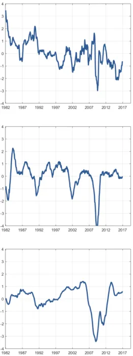
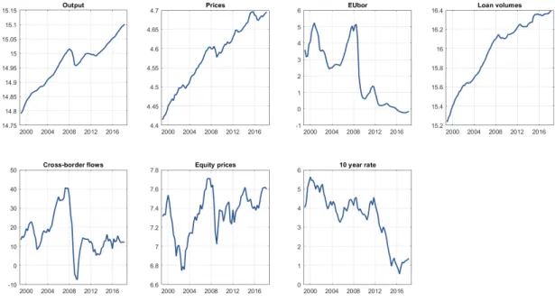
The baseline specification for inflation forecasting that I start with is an ex-tremely simple direct model which only includes lagged inflation. I then consider adding different macroeconomic variables to this specification in turn. The macroe-conomic variables that I use include monthly measures of inflation cycles, business cycles and financial cycles; all of which are factors estimated with principal compo-nents from many underlying indicators. They also include information on exchange rates, wages and monetary shocks. They therefore include equivalents of all of the variables traditionally used for forecasting discussed by Stock and Watson (2008) and cover many of the main series typically used in macroeconomic models.
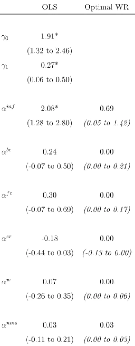
I estimate the true association between each variable and future inflation by adding each variable to the baseline case in turn and estimating the model with ordinary least squares (OLS). I estimate the association between each variable and future inflation that is optimal to use in forecasting as follows. I split the sample into many overlapping training sets and in each of them consider the model with each variable included in turn. However in each case I estimate the model many times using weighted ridge and applying different levels of shrinkage. The most shrunken case corresponds to estimating the baseline case with OLS and the least shrunken case corresponds to estimating the model with a specific variable included with OLS. I then take the optimal association between each variable and future inflation to use in forecasting as the one given by the level of shrinkage that minimises measures of forecast error in the test sets. The difference between the estimated optimal asso-ciation for forecasting and the estimated true assoasso-ciation for each macroeconomic variable is the estimate of the conditional bias applied to that variable by using optimal forecasts.
shrinkage to many macroeconomic variables. Indeed, it is essentially optimal to only use information on past price changes when producing inflation forecasts, although in a non-naive manner that incorporates partial shrinkage. The results also show that several of the macroeconomic variables analysed have statistically and economically significant associations with future inflation. Together these results suggest that optimal inflation forecasts incorporate large conditional biases with respect to the information in common macroeconomic variables.
I then estimate the conditional biases in surveyed household inflation expecta-tions. I do this by comparing the estimated associations between each macroeco-nomic variable and future inflation produced using the method described above and the equivalent association between each macroeconomic variable and household fore-casts of future inflation. This involves adding each variable to the baseline case in turn and estimating the model with OLS but comparing the results produced when using future inflation or household forecasts of future inflation as the dependent variable. I find that most conditional biases in household forecasts are very simi-lar to the equivalent conditional biases in optimal expectations. However some are clearly mistaken: for instance households forecasts of inflation significantly rise with a fall in the financial cycle indicator, when they should fall. Household forecasts are also clearly beaten in terms of pseudo out of sample forecasting performance by the baseline empirical model, suggesting that they are not optimal feasible expectations. Therefore these results suggest that the optimal feasible inflation expectations, which are statistically simple, contain large conditional biases with respect to a set of major macroeconomic variables. They therefore appear to be very different to rational expectations given available macroeconomic data. Household inflation fore-casts appear to be well explained by a combination of optimal feasible expectations and behavioural errors that decrease forecast performance.
These empirical results and the underlying discussions suggest that important conditional biases are likely to be present in the optimal feasible expectations of many macroeconomic variables. This implies that agents learning optimally from macroeconomic data are generally likely to estimate expectations that are very dif-ferent from rational expectations. This is a very important result, as it undermines
one of the major arguments used to try and justify the rational expectations revolu-tion. This implies that we should generally conceive of macroeconomic expectations as optimal feasible inflation expectations with the addition of behavioural errors in settings in which agents don’t act optimally. This suggests that the many current models based on rational expectations or very minor deviations from them are likely to be seriously mis-specified. It also suggests promising areas for future research, such as examining whether optimal feasible expectations vary between individuals and applying this new type of expectations to different areas of macroeconomics. For instance, the supplement to this thesis contained in the first appendix suggests how optimal feasible expectations could contribute to cycles in asset prices.
The second chapter is titled ‘Asset price convergence, international asset holdings and the quality of financial integration’. In it I assess the quality of recent changes in financial integration between EU countries.
This chapter builds on the existing empirical financial integration literature. Many papers in this literature produce measures of financial integration in Europe based on the unconditional convergence of asset prices and/or the proportion of international assets held in portfolios: see Hoffmann et al. (2019) for an overview. However increases in these measures do not just capture increases in the policy definition of financial integration, i.e. reductions in international financial frictions that cause differences in access to or investment of capital on the basis of location (Coeure, 2013), they also capture changes in the different underlying risks factors of assets and aversion to them. Increases in policy financial integration are usually suggested to have economic benefits by improving the efficiency of capital alloca-tion and risk sharing (Baele et al., 2004). However, since empirical measures of financial integration do not just capture changes in policy financial integration, in-creases in them they may not indicate capital allocation and risk sharing benefits. Additionally, increases in measured financial integration, whether driven by policy financial integration or underlying risk components, might impose economic costs by increasing the risks of financial contagion and instability (Stiglitz, 2010).
As a result most policy papers that update financial integration measures have also begun to discuss the quality of changes in financial integration measures, i.e.
the extent to which financial integration is likely to have net economic benefits (European Central Bank, 2016; European Investment Bank, 2017). The chapter contributes to the existing literature by providing a methodology for statistically analysing three aspects of the quality of changes in financial integration measures that are discussed in the existing literature. These are: whether there are jointly driven changes in price and quantity measures of integration (Coeure, 2013), whether the changes in financial integration are permanent (European Investment Bank, 2019) and whether the changes in financial integration are robust to shocks that affect macroeconomic conditions (European Central Bank, 2018). It also contributes by applying this methodology to analyse the three aspects of the quality of financial integration changes in the EU since 2000 and so provides indirect evidence of the extent to which this integration is likely to have produced economic benefits.
To analyse whether price and quantity integration measures have a joint driver I need to construct a financial integration factor from both price and quantity in-dicators of integration. This is econometrically challenging, as I also need to allow for permanent changes in the factor that may cause non-stationarity and insert the factor into a system with macroeconomic and financial variables to analyse its response to shocks to macroeconomic conditions. Therefore I cannot use typical principal components methods, which require stationary variables. Maximum like-lihood methods, such as the Kalman filter, could overcome this issue but are com-putationally challenging given the number of parameters used, so I use a Bayesian approach. Specifically I jointly estimate a Bayesian financial integration factor from many price and quantity integration indicators and the dynamics of a vector auto-regressive system that includes macroeconomic and financial variables as well as the factor. This estimation is achieved using Markov chain Monte Carlo methods: specifically a Gibbs sampler with a Carter-Kohn step to generate the factor. Ap-plying this method to data for the EU yields a measure of financial integration that has large increases in the early 2000s but then plateaus and has primarily decreased since 2008, although has recovered a little in the last few years.
I then test the sign of the factor loadings on price and quantity integration indi-cators to assess whether there is a joint driver, test the size of the deterministic and
stochastic trend changes to assess the permanence of any increases in the indicator and use sign restrictions to test the extent to which shocks that affect macroeco-nomic conditions also affect integration. I find that the financial integration factor is a strong joint driver of a wide range of price and quantity measures of integra-tion. The factor loads particularly positively on virtually all integration measures in the bank lending, corporate bond and government bond markets, but loads far less strongly on indicators in equity markets. However the changes in the financial inte-gration factor are virtually all cyclical, as long-term cyclicality strongly outweighs deterministic and stochastic trends, and vulnerable to shocks to macroeconomic conditions, as virtually all sign identified economic shocks cause large corresponding effects on financial integration.
Therefore it appears that changes in financial integration are primarily cyclical and vulnerable to macroeconomic shocks. As a result, most changes in financial in-tegration in the EU since 2000 appear unlikely to have provided large net economic benefits: they actually appear most closely related to cyclical changes in the under-lying risks of European assets and aversion to these risks. These results only covers the relatively short period of time since the millennium, so it would be interesting to update the results in the future when the effects of major recent events such as Brexit and Covid-19 can be studied.
The third chapter is titled ‘Behavioural finance at home: house price cycles in the USA’. In it I primarily assess whether US aggregate house prices are equal to their fundamental value, allowing for the effect of search frictions and contractual rigidities in housing markets. I also analyse the proximal drivers of housing market cycles.
This chapter partly builds on the existing literature testing whether house prices are equal to their fundamental value i.e. the rationally expected discounted sum of their rents given the state of the macroeconomy (Glaeser and Nathanson, 2015), and hence whether they are efficient in incorporating information. The patterns of strong correlations and persistence in house price changes and excess housing returns, dating to at least Case and Shiller (1989) with updates surveyed in Ghysels et al. (2013), suggests that housing markets are not efficient, even given time-varying
risk aversion. Therefore house prices do not appear to always be given by their fundamental value. The literature also suggests that housing market frictions may struggle to explain the size and cyclicality of these correlations and behavioural explanations may be needed (Glaeser and Nathanson, 2015), although this is hard to prove absolutely.
This chapter contributes to this literature by introducing a test for whether house prices are consistent with always being equal to the fundamental value of housing, adjusted to account for contractual rigidities and search frictions in housing markets, based on the speed of the reaction of house prices to monetary shocks. Monetary shocks should have a clearly signed impact on the fundamental value of housing, even allowing for rigidities and frictions, as soon as contractual rigidities no longer bind. Survey data from Ellie May indicates that this should be at horizons of one to two months. I support this concept with two conceptual frameworks and refer-ences to existing empirical work on the relevant transmission channels of monetary shocks and the frictions in housing markets. Therefore reacting significantly to mon-etary shocks within two months is a necessary, although not sufficient, condition for changes in house prices to be entirely caused by changes in the fundamental value of housing. Whereas if house prices deviate from their fundamental values, for in-stance because agents either do not observe monetary shocks or do not incorporate information on monetary shocks into their expectations rationally, then house prices may react to monetary shocks far more slowly. This is because they would only re-act once easily observable, noticeable and understandable information on monetary shocks becomes available, possibly as the macroeconomic effects of the shock are felt. This chapter also has a secondary contribution, as it also uses a sign decom-position based on the conceptual frameworks to identify the relative importance of proximal drivers of housing market cycles.
The approach used in this test is closely linked to the empirical monetary policy literature that attempts to produce impulse response functions of variables, such as house prices, to monetary shocks. This chapter uses methods similar to those in Coibion et al. (2017) to implement the test but additionally contributes to this literature by focusing on the particular horizon of interest and by using controls,
both in the generation of the shocks and in the production of the impulse response functions, that are specific to housing markets.
Specifically I implement the test using narrative shocks in the style of Romer and Romer (2004). However I include financial controls in the generation of the shocks to avoid any remaining endogeneity from central bank reactions to the strength of policy transmission as a result of financial conditions, which might be particularly important for an asset price like real house prices. I then use these shocks in a local projections approach that also includes housing specific controls, to obtain more accurate estimates. The local projection approach also means that the timing of responses can be directly estimated and so more accurately assessed than in indirect auto-regressive models.
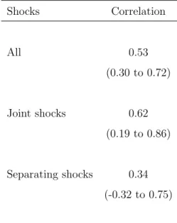
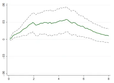
The results show that there is no statistically or economically significant reac-tions of aggregate US real house prices to monetary shocks at either one or two month horizons. However impulse response functions show that there are significant reactions with plausible signs at horizons greater than a year. In particular a one percentage point reduction in the base rate is estimated to cause an increase in real house prices of approximately three percent after two years, but virtually no effect at long horizons. Therefore these results show that aggregate real house prices in the US fail the test of consistency.
I also implement a sign decomposition based on the conceptual frameworks to identify the relative importance of proximal drivers of the cyclical component of house prices. Empirically I use band-pass filters to identify the cyclical components of house price variables and then calculate the linear and rank correlations between them. There are strong positive correlations between the cyclical components of real house prices and housing starts, but only limited associations between either of these variables and the cyclical component of real rents. Therefore the frameworks suggest that changes in consumption demand are the most important proximal driver of house price changes, changes in asset demand are also relatively important and changes in housing supply are the least important.
The slowness of the response of real house prices to monetary shocks suggests that house prices are not consistent with always being equal to the fundamental
value of housing, even after this is adjusted for search frictions and contractual rigidities. Therefore this suggests that either agents do not observe information on shocks well or that they do not use this information rationally. Both are plausible, as even experts struggle to measure macroeconomic shocks and understand their effects (Ramey, 2016). On the basis of these results investors and policymakers should con-ceive of housing cycles as being the partly behavioural response of housing markets to shifts in housing demand. This suggests that current macroeconomic models of housing markets based on the actions of agents using rational expectations with full information on macroeconomic shocks may be seriously mis-specified. Future work should instead focus on incorporating the behavioural nature of housing markets into macroeconomics.
The first appendix is titled ‘Behavioural financial cycles as the cause of perpetual business cycles’ and is a supplement to the three main chapters. In it I draw on the ideas from the chapters and the wider behavioural finance literature to produce a conceptual framework showing how a realistic financial cycle that is hard to predict can cause a perpetual business cycle. This behavioural financial cycle is caused by agents who use optimal feasible expectations, as introduced in Chapter 1, and have time-dependent fear-based preferences over risk, which Guiso et al. (2018) provides evidence for. The behavioural financial cycle permanently fluctuates in a stochastic way and, through its effects on aggregate demand, causes a perpetual business cycle. The other three appendices contain additional information and robustness checks for each of the three main chapters.
The three chapters are linked by a subject area and a methodological approach. The methodological approach I use in this thesis is based on the fundamental sci-entific and statistical principles outlined in Box (1976). Firstly, scisci-entific models typically have to be simplified versions of reality and so should seek to be at the efficient frontier of the trade-off between simplicity and realism. Secondly, the more approximations the model makes, the more approximate its conclusions must be: a highly realistic model can offer precise conclusions, whereas a stylised simplified model should only offer approximate ones.
realistic for their level of simplicity. However, since they are relatively simple, they can only offer approximate conclusions which, in turn, can provide a framework for empirical work. This empirical work is based on a range of methods including natural experiments, surveys, sign restrictions, forecasting analysis and informative associations. This work is conducted with the aim of providing more precise quan-titative answers to the questions addressed and therefore makes up the majority of the thesis.
This approach contrasts dramatically with the dynamic stochastic general equi-librium approach that dominates macroeconomic research in most academic institu-tions (Stiglitz, 2018). The dynamic stochastic general equilibrium approach uses far more complex and opaque models than my conceptual frameworks: typically taking many pages of calculus to derive and requiring software to solve. However these models are still very unrealistic, as they are based on very specific behaviour that contravenes important facts: a phenomenon which leads Romer (2016) to describe them as ‘post-real’ models. The clearest, but by no means only, example of this is that these models are built on the assumption that agents perfectly maximise util-ity functions using rational expectations, or minor deviations from such behaviour. This is despite the fact that the majority of people cannot correctly answer three extremely basic questions on economic and financial literacy: for instance in the United States only 34.3% of surveyed individuals were able to do so (Lusardi and Mitchell, 2014). Therefore, despite their complexity, these models are sufficiently unrealistic in important ways that one cannot be confident in either their precise or their approximate conclusions.
The three chapters also all analyse topics related to behavioural macro-financial cycles. More precisely, they each examine an aspect of the cyclical behaviour in an entire financial market, or group of markets, and its interaction with macroe-conomic variables. These interactions can either concern the effects of macroeco-nomic variables on financial cycles or the effect of financial market cyclicality on the macroeconomy. In either case there is also typically a focus on analysing the role of behavioural phenomena.
they all involve the measurement of financial cycles. In Chapter 1 I combine many indicators to develop financial cycle and business cycle indices using principal compo-nents; in Chapter 2 I combine many indicators to create an EU financial integration index and analyse its cyclical component in a Bayesian setting and in Chapter 3 I use band-pass filters to obtain the cyclical components of US housing market variables. Secondly, they all concern either the effect of financial cycles on macroeconomic variables or the effect of macroeconomic variables on financial cycles. In Chapter 1 I analyse the effects of financial cycles, amongst other variables, on inflation ex-pectations; in Chapter 2 I estimate the effect of shocks that affect macroeconomic conditions on cyclical financial integration and in Chapter 3 I estimate the effects of monetary shocks on real house prices and estimate the relative importance of the proximal economic drivers of housing cycles. Thirdly, they all focus, at least partially, on the role of behavioural phenomena, in particular expectations and risk aversion. In Chapter 1 I show that optimal feasible inflation expectations in the real world are substantially different from rational expectations and examine the rationality of household inflation forecasts. Chapter 2 does not directly analyse behavioural phenomena, but cyclical behavioural risk aversion is suggested as one of the drivers of cyclical changes in European financial integration. In Chapter 3 I show that the effects of monetary shocks on real house prices are not consistent with house prices being equal to their fundamental value, even allowing for housing market frictions, in a way that suggests that agents do not have full information rational house price expectations.
Chapter 1
Optimal feasible expectations in
our uncertain economy
1.1
Introduction
Understanding inflation expectations is central to macroeconomics. Inflation ex-pectations drive inflation itself through wage bargaining and price setting, so affect nominal rigidities and the response of the real economy to aggregate demand shocks. Therefore the responsiveness of inflation expectations to available information on macroeconomic shocks affects the answer to crucial questions such as the reaction of unemployment to financial crises or the ability of government spending to boost output.
Rational expectations have been the most common approach to modelling how inflation forecasts are formed in academic economics in recent years, although em-pirical and theoretical work has suggested behavioural alternatives (Coibion et al., 2018). They are defined as agents’ expectations being the conditional expectation of future variables, conditioning on available information1. Sheffrin (1996) provides a
full mathematical definition of this while the original definition is available in Muth (1961). They imply that agents’ expectations should react to publicly available
1Full information rational expectations, as described by Coibion et al. (2018) and commonly
used in academic macroeconomics, also require that complete knowledge of the economy is avail-able.
information in the same manner as future realised inflation reacts (Lovell, 1986). Rational expectations given available information will not always be the optimal feasible expectations for agents when forecasting a variable. If rational expectations are feasible then they will be the optimal feasible expectations for an agent, using mean square forecast error to define optimality (Diebold, 2017). However they will only be feasible if the agent can either deduce or perfectly estimate the relevant parameters of the conditional distribution of the variable being forecasted. Given the complexity of modern economies it is simply not possible to deduce rational expectations without estimation from data in the vast majority of circumstances. Therefore estimation from data must be used to form expectations. This has driven a large learning literature studying whether expectations based on learning from data converge to rational expectations, which is surveyed by Evans and Honkapohja (2012). Since papers in this literature are primarily interested in convergence, they often assume agents have access to infinite observations of data. With infinite data an agent can use a conditionally unbiased and consistent estimate as the conditional expectation, such as that formed by approaches similar to regressing realised values of the variable being forecast on all available past information. Such an approach would converge to the conditional expectation, i.e. rational expectations, so rational expectations are feasible with infinite data.
However with a finite series of data rational expectations are not generally feasi-ble, as conditionally unbiased estimators, such as those produced by regressing the variable being forecast on past information, will vary slightly around the conditional expectation as a result of estimation error. Any conditionally biased estimator will also contain clear deviations from rational expectations. Therefore rational expecta-tions will not be the optimal feasible expectaexpecta-tions in most settings. It also may not be optimal to try to limit the conditional biases that one imposes in expectations to make estimating them feasible. This is because it may be worth shrinking estimated expectations towards statistically simple expectations to reduce forecast variance, even though this introduces greater conditional biases. This insight is at the heart of modern machine learning (Ahmed et al., 2010) and Bayesian approaches to fore-casting (De Mol et al., 2008) and is also present in frequentist forefore-casting approaches
(Bai and Ng, 2008).
I begin this chapter by discussing why some shrinkage is likely to be needed when forming expectations for the vast majority of macroeconomic variables, as a result of the large number of potentially relevant data series available relative to the number of observations of each series2. I also discuss why it is very often likely
that additional shrinkage towards statistically simpler specifications will improve the bias-variance trade-off of forecasts as a result of reducing estimation error and so reduce measures of forecast error. However the precise level of shrinkage in optimal feasible expectations in a particular setting is ultimately an empirical issue, so I then analyse the empirical importance of this shrinkage when forecasting US inflation.
Specifically I consider adding a number of different potential predictors of infla-tion to a baseline auto-regressive forecast of inflainfla-tion. I estimate these forecasts in a number of training sets using weighted ridge specifications with different levels of statistical shrinkage applied to each additional predictor and then take the optimal degree of shrinkage as the one which minimises measures of forecast errors in test sets. The results suggest that a large degree of shrinkage should be applied to most variables3; indeed the optimal forecast virtually only uses information on past
infla-tion and components of inflainfla-tion. These results are closely linked to those from the empirical inflation forecasting literature, which show that univariate inflation fore-casts are hard to beat in forecasting horse-races (Stock and Watson, 2008). However, unlike this literature, I also estimate equivalent specifications without shrinkage and find that inflation does have economically and statistically significant associations with some of the predictors. This implies that the high levels of optimal shrinkage do not just come from inflation being uncorrelated with past information, they also come from it being worth conditionally biasing inflation forecasts towards statisti-cally simpler forecasts to reduce conditional forecast error. Therefore the optimal feasible inflation expectations are very different from rational expectations.
Finally I analyse the conditional biases in surveys of actual US household
in-2A phenomenon known as fat data (Koop, 2017)
3The results only consider the linear effects of the variables, but given the number of potential
non-linear effects far more shrinkage would be needed to even make estimation with a wide range of non-linear effects feasible.
flation forecasts using an approach similar to that in the existing literature. I find that there are significant biases, particularly in the response to changes in past broad inflation and to financial cycle indicators. Many of these conditional biases appear to arise from using the same conditional biases as estimated optimal feasible expectations, such as the limited response to broad changes in past inflation. How-ever household forecasts are shown not to be the optimal feasible expectations, as they perform worse in pseudo out of sample forecast comparisons than feasible em-pirical alternatives4. Therefore both optimal feasible expectations and behavioural
mistakes are likely to have a role in explaining US household inflation forecasts. I also suggest optimal feasible expectations as a new general class of expec-tations, formally defined as the expectations that are predicted to minimise the relevant measure of forecast error out of the set of expectations that it is feasible for agents in the real world to estimate. Optimal feasible expectations are likely to differ materially from rational expectations in most circumstances as they are likely to incorporate conditional biases associated with being statistically simple. Indeed, given the importance of parsimony in forecasting many variables (Kim and Swanson, 2018), despite their no doubt numerous true links to one another, optimal shrinkage is likely to cause optimal feasible expectations to be dramatically differ-ent to rational expectations in a large number of macroeconomic settings. I suggest that we should generally conceive of macroeconomic expectations as optimal feasible inflation expectations with the addition of behavioural errors in settings in which agents do not act optimally.
Work on how inflation expectations are formed has a long and important history in the macroeconomic literature that includes the discussions of money illusion in Keynes (1936), the adaptive inflation expectations in Friedman (1977), the model-specific rational price expectations in Lucas (1996) and the behavioural pricing in Akerlof (2002). However the work in this chapter is most closely related to, and contributes to, three relatively distinct branches of the existing literature.
Firstly, this chapter relates to the literature studying learning and expectations
4This is unsurprising given the clear evidence that many people have a poor understanding of
in macroeconomics, as surveyed in Evans and Honkapohja (2012). In this literature work tends to investigate the implications of agents learning expectations from data in theoretical macroeconomic models. As the majority of this literature tends to focus on whether such learning behaviour leads to models converging to rational expectations equilibria, it is common practice to assume that agents have access to an infinite series of relevant data (Evans and Honkapohja, 2012). However, as de-scribed above, in this case it is feasible and optimal to use a conditionally unbiased and consistent estimate of rational expectations, such as that given by approaches based on least squares, which then simply implies that agents use rational expecta-tions5. When agents have finite data it is not feasible to use rational expectations, as
consistent estimators will not converge to the true conditional expectations. How-ever it may be possible to use a conditionally unbiased estimator, such as approaches based on least squares similar to that in Orphanides and Williams (2007), which im-plies that agents use rational expectations plus noise. However the papers that are most closely related to this chapter are those in which agents with finite data use methods that give conditionally biased expectations. For instance Hommes et al. (2019) assume agents use least squares but only applied to an auto-regressive rule while Chung and Xiao (2013) assume that agents use a vector auto-regression with a subset of relevant variables.
The justification for these learning methods is that the authors are looking for a method that balances tractability in the theoretical model considered with being a good approximation for what some forecasters do in practice. I contribute to this literature by studying the optimal expectations that are feasible for an agent to use, rather than the feasible expectations that some agents may use in practice. My em-pirical approach frees me to do this and has the advantage of allowing me to study shrinkage in the real world. I demonstrate that in the case of US inflation forecast-ing the optimal feasible expectations contain large conditional biases, conditionforecast-ing on important macroeconomic series and series that are often used as predictors of
5Note I am discussing whether an approach implies that agents use rational expectations from
an infinite sample of relevant data, not whether an approach leads to a specific model converging to a rational expectations equilibria of that model.
inflation. This is because shrinking expectations towards simpler forecasts reduces conditional forecast variance sufficiently to more than offset the conditional forecast bias imparted. I also suggest why similar shrinkage is also likely to be used in the optimal feasible expectations in the vast majority of macroeconomic settings. This is hugely important as it implies that agents learning optimally will use expectations that are often very different from rational expectations, despite this being a funda-mental justification of the rational expectations revolution (Coibion et al., 2018). I therefore suggest optimal feasible expectations as a new general class of expectations that are defined as the expectations that have the lowest predictable forecast error out of the set of expectations that agents in the real world could actually estimate. These are likely to be conditionally biased towards statistically simple specifications, so will usually be much statistically simpler than rational expectations.
Secondly, this chapter relates to the econometric literature on forecasting infla-tion. There are a very large number of papers that analyse different approaches for forecasting inflation, in terms of method and/or predictive variables, and compare pseudo out of sample forecast error measures. Reviews of this literature are pro-vided for traditional econometric methods in Stock and Watson (2008) and Faust and Wright (2013), while Medeiros et al. (2020) extend this analysis to machine learning methods. A key message that emerges from these reviews is the importance of par-simony. Simple auto-regressive benchmarks forecast extremely well: they are hard to consistently out-perform and effectively impossible to consistently out-perform by a large margin at horizons less than two years. Those methods that do appear to out-perform them minimise and constrain additional estimation. These include factor models with a very limited number of macroeconomic factors (Stock and Wat-son, 2002), extensions to benchmark models that still only use price data but allow different components of inflation to have different effects (Stock and Watson, 2016) and very heavily pruned random forests that allow some heavily constrained effects of employment variables (Medeiros et al., 2020). Theoretical restrictions derived from DSGE models are not useful for improving forecasting performance (Giaco-mini, 2015), however central banks targets, or proxies for them, become the optimal forecasts at horizons much beyond two years (Faust and Wright, 2013). This
ap-pears sensible, as central banks aim to target inflation in the medium term, however at horizons of two years or less lags in the effects of monetary policy (Havranek and Rusnak, 2013) and central banks’ preferences for gradual adjustment of interest rates (Coibion and Gorodnichenko, 2012b) suggest that inflation deviations from targets are forecastable.
This literature currently does not address precisely why it is not optimal to add information on particular variables to auto-regressive benchmarks and I contribute to this literature by studying why this is the case. I initially assess how much shrinkage is optimal to apply to a series of macroeconomic variables, that include the main variables often used in macroeconomic models and variables commonly used in inflation forecasting. In line with the existing literature I find that the majority of variables should have total shrinkage applied to them, implying that one should virtually only use information on price series to form inflation forecasts. This information should not be used naively though, as different types of inflation should be allowed to have effects that differ but are constrained to limit estimation error. However I go on to provide the first comparisons of the shrunken estimates of the association between each variable and future inflation that is optimal for forecasting and consistent OLS estimates of the equivalent actual association. This allows me to analyse whether the high optimal degree of shrinkage comes from the variables simply not having much of an association with future inflation or from the benefits of reducing the variance of the forecast despite this imposing conditional biases because the variables having strong associations with future inflation. The results suggest that for many variables, such as broad inflation and measures of business and financial cycles it is the former, although for variables like wages it is the latter. This is important as it suggests that it is primarily the high degree of uncertainty over the associations between some variables and future inflation that prevents them from being useful in forecasting inflation, rather than the variables simply not having much association with future inflation.
Thirdly, this chapter relates to the literature which tests for conditional biases, and hence deviations from rational expectations, in surveys of agents inflation ex-pectations. The main method of testing this in the literature, and the approach
used in this chapter, is to test whether inflation forecasts and future realised infla-tion react differently to informainfla-tion that was publicly available at the time of the forecast. Coibion et al. (2018) surveys papers that take this approach. Variables that have been suggested to cause a different response in forecast and realised in-flation include lagged forecast errors (Coibion and Gorodnichenko, 2015a), lagged changes in exchange rates (Pesaran and Weale, 2006), narrative shocks (Coibion and Gorodnichenko, 2012a) and lagged energy components of inflation (Coibion and Gorodnichenko, 2015b). Understanding which variables there is a conditionally bi-ased reaction to is important, as this determines which nominal rigidities occur and so helps us to understand how large the nominal rigidities are for the transmission mechanisms of different macroeconomic shocks.
Suggested explanations usually focus on non-optimal behaviour6, often
result-ing from some combination of rational inattention or imperfect understandresult-ings of the economy (Coibion et al., 2018). This must be at least partly true, as Berge (2018) shows that agent’s inflation forecasts can be beaten in pseudo out of sample forecasting by simple auto-regressive moving average models that would have been feasible for agents to use. However it is very important to understand whether some of the specific conditional biases actually arise from optimal feasible behaviour, and so could not be corrected, or if they all arise from potentially correctable behavioural errors. I contribute to this literature by providing what, to my knowledge, is the first evidence on this issue. Using methods similar to the existing literature I es-timate the conditional biases in surveys of US household inflation forecasts with respect to a set of macroeconomic variables and show that household forecasts are not optimal feasible expectations as they can be beaten by simple auto-regressive benchmarks. However unlike the existing literature, I then go on to compare the conditional biases in household forecasts to the conditional biases in estimated opti-mal feasible expectations. I find that the conditional biases in the reaction to many variables, such as broad and narrow inflation, business cycles and exchange rates,
6Explanations for some variables, such as aggregate forecast revisions, also include that
infor-mation on them might not be available in real time, but this is not an issue in this chapter as we only consider variables that are publicly available.
are consistent with suggested optimal feasible behaviour. However the reaction to financial cycle information and the amount of noise in household inflation forecasts do not appear to be consistent with optimal feasible behaviour and instead sug-gest behavioural mistakes. Therefore optimal feasible expectations and behavioural mistakes are each likely to explain part of US households’ inflation forecasts.
The rest of the chapter is organised as follows. Section 1.2 lays out my conceptual and econometric framework, Section 1.3 describes the macroeconomic information used and how I combine some of this information into factors, Section 1.4 presents the estimates of the conditional biases in optimal feasible inflation expectations, Section 1.5 estimates the conditional biases in surveys of household inflation expec-tations and compares these to the estimated optimal conditional biases and Section 1.6 offers some concluding remarks.
1.2
Conceptual and econometric setup
To clarify the definitions that follow I begin by decomposing future inflation into a component based on public information that is currently available and a component that is unrelated to this information. I then also express forecast inflation in terms of public information that is currently available, as follows:
πr t+h =xtβr+t+h (1.1) πtf+h =xtβf (1.2) whereπr t+h is inflation at timet+h,π f
t+h is an agent’s forecast at time tof inflation
at time t+h, xt is a vector of information that is publicly available at time t, βr
is a vector of true coefficients, βf is a vector of coefficients that agents use in their
forecasts and t+h is the component of inflation at time t+h that is unpredictable
a timet with public information.
This expression is very general, asxtcould include lagged information or
informa-tion which is non-linear in underlying indicators. It could also include informainforma-tion that is unrelated to future inflation, so that some of the values inβr could be zero.
The definitions of the terms used are then as follows. I define the set of feasible expectations as expectations based on choices of βf that agents can actually use
in realistic settings. For instance it would be feasible to use OLS to estimate the values based on past observations. It would also be feasible to choose to set the value on lagged inflation to one and all other values to zero. I define optimal feasible expectations as the specific expectations in the set of feasible expectations that ex ante can be predicted to minimise the relevant measure of out of sample forecast error. Rational expectations are defined following Sheffrin (1996), and originally Muth (1961), as expectations that are equal to the true conditional expectation of future variables, conditioning on available information. Applying this definition in this settings yields that rational expectations are the expectations given when βf =βr.
I now consider whether rational expectations will be the optimal feasible expec-tations in realistic settings. First it is important to note that if rational expecexpec-tations are feasible then they will be optimal, as defined by the mean square forecast error7,
since the conditional expectation statistically minimises mean squared forecast error (Granger and Newbold, 1986). If an agent had infinite relevant data to learn from then they could use any consistent estimator ofβr to obtain an estimate essentially
equal to βr that could then be used to construct rational expectations8. For
in-stance one could use past observations to estimate Equation 1.1 using OLS with all potential predictors of inflation inxtto obtain an estimate ofβr that is statistically
perfect. The agent could then use this perfect estimate ofβr as βf, so rational
ex-pectations are feasible in this scenario and hence they are also the optimal feasible expectation.
However in reality, agents clearly only have a finite sample of data available to them. Forecasts often need to be constructed at horizons of at least a year, however samples of relevant data are usually short relative to these horizons and will not
7A single point forecast can only generally minimise a single forecast accuracy measure and the
mean square forecast error is one of the most common measures Diebold (2017).
8Technically this applies to stationary variables. One would need to difference non-stationary
variables until stationarity was achieved before applying this process. Then the results of this process and the current values of the variables could then be used to construct rational expectations.
necessarily increase over time, as economies experience huge structural changes that decrease the relevance of older data. For instance, formal tests (Stock and Watson, 1996) and institutional change suggest that the economic dynamics of countries now are very different from the dynamics in the period before the 1980s, when most policymakers were fully Keynesian and the internet had not yet been invented. They are likely to be even more different to the dynamics from earlier periods when many of these countries engaged in active global wars with one another. Therefore data from previous structural eras is unlikely to be of significant quantitative relevance for an agent seriously engaged in inflation forecasting (Stock and Watson, 2008). There are also strong reasons to believe that this phenomenon will continue in the future. For instance it seems extremely likely that there will be significant structural economic change as a result of the rise of artificial intelligence, new shocks such as Covid-19 and the increased economic importance of countries like China.
In reality there are huge number of potential predictors that are likely to have some effects on inflation relative to samples of data of these lengths9, as any variable
that affects how firms set prices will have some effect on future inflation at shorter horizons. Combining similar variables may reduce the number of series that could be used but lags and non-linear transformations will increase this number and it will remain very large in practice. For instance Refinitiv Datastream and similar services provides millions of macroeconomic data series yet even samples dating to World War 2 only contains hundreds of months of observations. Therefore using condi-tionally unbiased approaches is simply not feasible. For instance, OLS estimates of Equation 1.1 cannot be estimated while including many of the macroeconomic series that are available. Therefore agents will generally need to use an estimation approach that shrinks forecasts, partially or even absolutely, towards statistically simpler specifications for estimation to be feasible. This implies that in practice all feasible expectations are likely to contain conditional biases, so rational expectations will not be feasible.
Even if one had incorporated enough shrinkage to make estimation feasible it
9A phenomenon that has been more broadly been described as big data in macroeconomics
may well be optimal to include more shrinkage. The optimal feasible approach needs to optimally balance conditional forecast bias against conditional forecast variance, conditioning on the information available. This can be seen most clearly when using the mean squared forecast error as the measure of forecast performance. Consider the following decomposition of the mean squared forecast error, where all expectations are conditional on the information in xt and the decomposition uses
Equation 1.1, into the components that contribute to it:
M SF E =E(πtf+h−πrt+h)2
=E(t+h)2+E(xtβf −xtβr)2−2E(t+h(xtβf −xtβr))
=E(t+h)2+E(xtβf −E(xtβf) +E(xtβf)−xtβr)2
=E(t+h)2+E(xtβf −E(xtβf))2+ (E(xtβf)−xtβr)2
=unpredictable component + f orecast0s variance + (f orecast0s bias)2 (1.3) The choice of the parameters,βf cannot change the unpredictable component but
they will affect the conditional variance and the conditional bias. An approach that is just feasible, such as using OLS estimates of Equation 1.1 with as many series inxt
as observations may minimise conditional biases, but is also very likely to impart a large amount of estimation error that contributes to conditional variance. Whereas using an approach that did not involve estimation, such as assuming a random walk, would minimise conditional variance but is very likely to impart conditional bias. Therefore there is typically a bias-variance trade-off to consider in the choice of how much shrinkage an agent should use when choosingβf.
The statistically simple specifications that it is optimal to shrink forecasts to-wards will not usually be given by theoretical macroeconomic models. On a purely empirical level this is currently true, as the literature survey in Giacomini (2015) shows that the full results of quantitative macroeconomic models are not useful for improving the forecasts of typical macroeconomic variables given by purely statisti-cal approaches. Giacomini (2015) suggests that the limited results to the contrary
are a product of the data mining that is fundamental in creating a theoretical model of an economy based on recent experience and then testing its ability to forecast in a sample that includes the periods on which recent experience is based. On a more fundamental level it is likely to continue to be true as theoretical macroeconomic models usually only offer predictions conditional on structural shocks and state vari-ables that are not well observed in practice (Chung and Xiao, 2013), so proxies for them may not have the predicted effects.
There are a limited number of cases where useful guesses of coefficients in βf
can be deduced without data10, some of which are discussed in Giacomini (2015).
In a very limited number of cases these may even allow expectations that are close to rational to be used: for instance heavily shrinking long-term inflation forecasts in some countries towards the countries inflation target. However in the vast ma-jority of cases where there is no such information available the natural choice to shrink coefficients in βf towards is zero. The optimal degree of shrinkage can then
be based on a combination of how relevant an agent thinks a variable is likely to be, for instance ruling out variables that are likely to have little association with the macroeconomy in question so are unlikely to have large effects, and empirical methods, such as pseudo out of sample tests or Bayesian model averaging.
I therefore suggest a new class of expectations: optimal feasible expectations. These are formally defined as the point expectations that are ex ante predicted to minimise the relevant measure of forecast error out of the set of expectations that it is feasible for agents to use in practice11. Based on the above discussion I suggest
that in the vast majority of macroeconomic settings optimal feasible expectations are likely to be statistically simpler than rational expectations, as many variables effects will be shrunk significantly towards zero, so they will generally incorporate
10However shrinking coefficient towards these values may actually increase the degree of shrinkage
in optimal feasible expectations relative to shrinking them towards zero, as the same reduction in conditional forecast variance from absolute shrinkage could then be achieved with less conditional bias.
11Optimal feasible expectations could therefore vary for different agents if they aim to minimise
sufficiently different measures of forecast error in the same setting. However this is partly a product of analysing point forecasts and is not the focus of this paper, so is not explored here.
conditional biases. However the exact size of the conditional biases in optimal feasible expectations, and hence their differences with rational expectations, is an empirical question. It depends on the degree of shrinkage that is optimal to apply to variables that have large associations with future inflation. I therefore now turn to examining the degree of optimal shrinkage to apply to variables in US inflation forecasting. The specific variables I choose are ones that are thought to transmit shocks to inflation in many macroeconomic models and so have long been suggested in the literature as potentially having associations with future inflation.
It is worth noting however that even if empirically observed shrinkage is rela-tively small this could imply large deviations from rational expectations equilibria, as it may represent the endpoint of a feedback loop. For instance, consider agents applying shrinkage with regards to information on a macroeconomic shock, so that their expectations responded less than rational expectations would to information on the shock. This could in turn reduce the response of realised inflation itself to the shock, relative to rational expectations equilibria, which could lead to even greater differences between expectations and those in rational expectations equilibria, cre-ating a feedback loop. Therefore actual data may be generated by the end point of such a feedback loop and relatively limited empirical shrinkage could still imply large nominal rigidities relative to comparable rational expectations equilibria.
Since estimating without shrinkage is infeasible in reality, as discussed above, I start with an extremely parsimonious specification and then consider how much it is worth shrinking the effects of additional macroeconomic variables that are added to this benchmark12. As well as estimating the degree of shrinkage that is optimal
to apply to the predictive associations of each of these variables when forecasting future inflation, I also estimate the true association between each variable and future inflation. This lets me analyse the size of the conditional biases present in the estimated optimal feasible inflation expectations.
The baseline specification that I start with is an extremely simple direct auto-regressive model estimated by OLS. It simply expresses inflation at timet+h,πr
t+h,
12This also seems sensible given the importance placed on extreme parsimony by the inflation
in terms of inflation at time t, πr
t, and a constant:
πtr+h =γ0+γ1πrt +εt+h (1.4)
I can then consider the optimal level of shrinkage to apply to additional macroe-conomic variables13 using pseudo out of sample inflation forecasting performance.
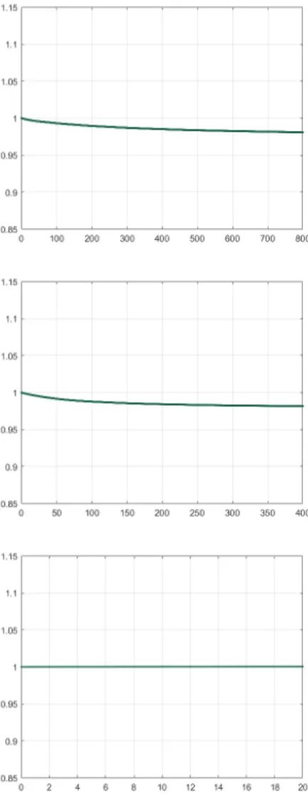
To do this I take many overlapping sub-samples from my sample and then in each of these training sub-samples calculate estimates of the coefficients on these addi-tional variables with different levels of shrinkage. The optimal level of shrinkage can then be taken as the one which minimises the pseudo out of sample forecasting error from the remaining test datasets. The approach is therefore a conservative one for estimating the optimal degree of shrinkage, as a new test set is not used for every variable. This pseudo out of sample approach is a common method of setting the level of shrinkage in machine learning approaches such as those in Medeiros et al. (2020). Note that the optimal level of shrinkage will become very small as the sample becomes very large, so this approach can still produce a consistent forecast. I implement the shrunken estimates using weighted ridge regression14, which can
shrink different coefficients by different quantities and can be expressed as a linear transformation of OLS so can be calculated analytically. I only apply shrinkage to the additional variable that is included. Weighted ridge regression minimises a loss function which combines the OLS loss function with a quadratic penalisation term, so the WR loss function and the OLS loss function can be expressed as follows:
Loss F unctionW R = (Π−Xβ)0(Π−Xβ) +β0Λβ (1.5)
Loss F unctionOLS = (Π−Xβ)0(Π−Xβ) (1.6)
13These variables are only included in linear form, which is conservative as there are so many
potential non-linear transformations of variables that attempting to include all of them would require the use of significant shrinkage for estimation to be feasible.
14Given the maximum number of variables considered is low, there is little difference between
the forecasts produced with this method and alternatives such as lasso or elastic net shrinkage. However there is an analytical solution for weighted ridge, unlike for lasso or elastic net penalisation, making the bootstrapping process used dramatically faster.
where Λ is a diagonal shrinkage matrix in which the values corresponding to the con-stant and lagged inflation are zero while the value corresponding to the additional variable considered is positive or zero, Π is the vector formed by stacking the de-pendent realised inflation variable, X is the matrix formed by stacking independent variables andβ is the vector formed by stacking coefficients.
Therefore, for each additional variable considered, I estimate the following speci-fication by OLS for the whole period and by a series of weighted ridges with multiple levels of shrinkage over each of a series of training periods for each additional variable vi:
πtr+h =γ0+γ1πtr+αvti+εt+h (1.7)
In all specifications I shrink the coefficient on the additional variable included towards zero as a neutral choice and apply no shrinkage to the mean and auto-regressive term. The out of sample forecasting results with different levels of shrunken coefficients then provide estimates of the optimal level of shrinkage to be applied to different key v