Forecasting Value-at-Risk under temporal and portfolio aggregation

TI 2015-140/III

Tinbergen Institute Discussion Paper

Forecasting Value-at-Risk under

Temporal and Portfolio Aggregation

Erik Kole

Thijs Markwat

Anne Opschoor

Dick van Dijk

REVISION APRIL 2017

1 _{Econometric Institute, Erasmus University Rotterdam} 2 _{Robeco Asset Management}

3 _{Vrije Universiteit Amsterdam} 4 _{Tinbergen Institute}

Tinbergen Institute is the graduate school and research institute in economics of Erasmus University Rotterdam, the University of Amsterdam and VU University Amsterdam.

Contact: [email protected]

More TI discussion papers can be downloaded at http://www.tinbergen.nl

Tinbergen Institute has two locations: Tinbergen Institute Amsterdam

Gustav Mahlerplein 117 1082 MS Amsterdam The Netherlands

Tel.: +31(0)20 598 4580 Tinbergen Institute Rotterdam Burg. Oudlaan 50

3062 PA Rotterdam The Netherlands

Forecasting Value-at-Risk under Temporal and Portfolio

Aggregation

*

Erik Kole

, Thijs Markwat

, Anne Opschoor

, and Dick van Dijk

2_{Robeco Asset Management} 3_{VU University Amsterdam}

4_{Tinbergen Institute}

5_{Erasmus Research Institute of Management}

April 19, 2017

Abstract

We examine the impact of temporal and portfolio aggregation on the quality of Value-at-Risk (VaR) forecasts over a horizon of ten trading days for a well-diversified portfolio of stocks, bonds and alternative investments. The VaR forecasts are constructed based on daily, weekly or biweekly returns of all constituent assets separately, gathered into portfolios based on asset class, or into a single portfolio. We compare the impact of aggregation to that of choosing a model for the conditional volatilities and correlations, the distribution for the innovations and the method of forecast construction. We find that the level of temporal aggregation is most important. Daily returns form the best basis for VaR forecasts. Modeling the portfolio at the asset or asset class level works better than complete portfolio aggregation, but differences are smaller. The differences from the model, distribution and forecast choices are also smaller compared to temporal aggregation.

Key words: forecast evaluation, aggregation, Value-at-Risk, model comparison JEL classification: C22, C32, C52, C53, G17

*_{The authors thank Fabio Trojani (the editor), the associate editor and two anonymous referees, as well} as participants at the 9th Annual SoFiE Conference in Hong Kong 2016, the 3rd Annual IAAE Conference in Milan 2016 and the Financial Econometrics and Empirical Asset Pricing Conference at the University of Lancaster 2016 for many helpful comments and suggestions.

„_{Corresponding Author: Erasmus University Rotterdam, P.O. Box 1738, NL-3000 DR Rotterdam, The} Netherlands. E-mail addresses are [email protected], [email protected], [email protected], and

1

Introduction

Value-at-Risk (VaR) for a horizon of ten trading days has become the standard downside risk measure for investment portfolios since the Basel Committee on Banking Supervision (1996), and is widely used in the financial sector (see Berkowitz and O’Brien, 2002). Because prices can be observed at a higher frequency and for all assets in the portfolio, a risk manager has to choose the degree of aggregation of the observations when constructing the VaR forecast. The typical approach in practice first gathers the assets into asset classes like stocks, bonds, and alternative assets. Next, a model for the daily asset class returns is used to construct a one-step VaR forecast for the portfolio. This forecast is then scaled to the required horizon by the square-root-of-time rule. This scaling of the daily VaR forecast is explicitly advised in the Basel Committee on Banking Supervision (1996) (see also Diebold et al., 1997; Dan´ıelsson and Zigrand, 2006). However, many alternatives with a lower or higher degree of temporal and portfolio aggregation are available.

We investigate the importance of the aggregation choice for the quality of ten-day VaR forecasts. This VaR forecast is a quantile of the portfolio return distribution over the coming ten days. We focus on the 1% and 5% quantiles, so VaR forecasts with 99% and 95% confi-dence levels. To construct this distribution, a risk manager can use different degrees of both temporal and portfolio aggregation. We compare their importance to other required choices. In particular, we consider different models for the conditional volatilities and correlations of the asset returns, different distributions for the innovations in these models, and different methods to construct cumulative multi-step forecasts (see also McAleer, 2009).

The degree of aggregation determines how detailed the serial and cross-sectional depen-dence of the returns is modeled. A model for all assets at the highest observed frequency describes very precisely how shocks to one particular asset affect its own future return dis-tribution at different horizons, as well as that of other assets. However, such an extensive model can be tedious to use in practice. Aggregation of assets into portfolios reduces the model dimension, whereas temporal aggregation reduces the number of forecasts that have to be accumulated. It also reduce the complexity of the model, if serial dependence only has short-term consequences.

Consequently, these choices involve a trade-off between precision and efficiency on the one hand and complexity and the risk of misspecification on the other hand. A low degree of aggregation particularly improves precision when different aspects of the return distributions

vary. For instance, when the effect of shocks on the volatility is more persistent in one (group of) asset(s), temporally and cross-sectionally aggregated models will lead to imprecise forecasts. Less temporal aggregation also increases the efficiency, since more observations are available (keeping the estimation window fixed). The flip side of this choice is the risk of misspecification. More complex models are generally less robust to misspecification. The effects of errors in the specification can be amplified by the forecasting horizon. Small errors in a single-period forecast can build up to a large error in a multi-step forecast.1

We study the impact of the degree of aggregation on ten-day VaR forecasts for a well-diversified portfolio of eight indexes, related to equities, bonds, and alternative assets. We vary the degree of temporal aggregation between modeling daily, weekly and biweekly re-turns, so from no to full temporal aggregation. In the cross-sectional dimension we analyze aggregation into a single portfolio, into the three main asset classes (stocks, bonds and al-ternatives), and no aggregation, so modeling the returns on all eight portfolio constituents. We examine all possible combinations of these different levels of temporal and portfolio ag-gregation. We do not examine the use of intraday data, because they are generally used in models for daily data (see, for example, Giot and Laurent, 2004; Clements et al., 2008; Brownlees and Gallo, 2010). Instead, we focus on methods that use one specific frequency. We leave a comparison of models that use mixed data frequencies with or without intraday data (see also Ghysels et al., 2009) for future research.

We compare the impact of aggregation to that of three other important required choices: the model for the conditional volatilities and correlations, the distribution for the innovations and the method of forecast construction. Regarding the first choice, we examine six well-established, relatively simple models from the GARCH family. We combine the univariate GARCH models of Bollerslev (1986) and Glosten et al. (1993) (GJR) with the CCC model of Bollerslev (1990), the DCC model of Engle (2002) and the rank-1 HDCC model from Bauwens et al. (2016) for the correlations. Hansen and Lunde (2005) and Laurent et al. (2012) show that these models perform just as well as more extensive alternatives (see, for example, Kuester et al., 2006; Brownlees and Gallo, 2010). The RiskMetrics approach from JP Morgan and Reuters (1996), which is popular in practice, completes the set of models. These seven models allow us to determine the importance of asymmetry in the marginal models and of dynamics in the correlations. The RiskMetrics approach offers a

one-size-1_{See the surveys by Bhansali (1999) and Chevillon (2007) for a general discussion of iterated versus direct}

fits-all alternative. As distributions for the innovations in these models we use a copula approach based on the normal, the Student’s t and the empirical distribution. While the failure of the normal distribution for risk measurement has been widely documented since Mandelbrot (1963) and Fama (1965), it remains popular in practice. The other two are promising alternatives.

The method of forecast construction is relevant when returns are modeled at a higher frequency than the forecast horizon. Cumulative multi-step forecasts can be constructed by an iterative procedure or by scaling one-step forecasts.2 In the iterative procedure, h-step forecasts are constructed by iterating forward the one-period-ahead density for h periods.3

This procedure captures the path dependence that the models imply, but can be time-consuming. A faster though perhaps less accurate alternative is the scaling of the one-period risk forecast. Scaling by the square-root-of-time is the industry standard, even though it can lead to overestimation of the ten-day VaR (see Diebold et al., 1997) as well as underestimation (see Dan´ıelsson and Zigrand, 2006; Wang et al., 2011).

The combination of these five choice aspects leads to 255 methods to forecast the VaR. We use the tests proposed by Christoffersen (1998) and Engle and Manganelli (2004) to assess the accuracy of each method in isolation. We examine whether a particular method outperforms another by constructing Model Confidence Sets as proposed by Hansen et al. (2011) based on the asymmetric tick-loss function as in Giacomini and Komunjer (2005). We also conduct pairwise comparisons based on the test of Diebold and Mariano (1995) in the framework of Giacomini and White (2006). These horse races are based on more than five thousand ten-day VaR forecasts for the period 1994–2014. We use the industry standard of a VaR confidence level of 99%, and use 95% as a robustness check.

Our results show that the degree of temporal aggregation is most important, whereas the degree of portfolio aggregation is less consequential. Working with daily returns leads to 99%- and 95%-VaR forecasts that come closest to having correct coverage, and perform significantly better than forecasts based on weekly or biweekly returns. While we also find evidence supporting more detailed multivariate models, in particular for 95%-VaR forecasts, differences here are smaller and in many cases not significant. Our results point at models based on the three main asset classes for 99%-VaR forecasts, and models on the asset level

2_{In specific cases, closed-form expressions for the multi-step distributions can be used. See for example}

Drost and Nijman (1993) for the GARCH(1,1) model, Hafner (2008) for multivariate GARCH models, and Sbrana and Silvestrini (2013) for the RiskMetrics method.

3_{See Marcellino et al. (2006) for iterated forecasts in an autoregressive framework and Ghysels et al.}

for the 95% case. We conclude that the methods with lower degrees of aggregation better capture the propagation of shocks, both over time and between the different asset returns.

When forecasts are constructed by iterating based on daily data, the GJR model of Glosten et al. (1993) gives the best forecasts, whereas the distribution choice is of less con-sequence. When forecasts are constructed from weekly or biweekly data, the distribution choice is important for 99%-VaR forecasts, but not for 95% forecasts. In the 99% case, the empirical (Student’s t) distribution performs best for weekly (biweekly) data. So, at the (bi)weekly frequency the innovations capture the fat tails and asymmetry, whereas the mo-dels incorporate these features at the daily frequency. The method of forecast construction is not that important. Our evidence tends to favor iterating over scaling to form forecasts, but differences vary widely based on the other settings. When combined with a normal distri-bution, scaling leads to worse performance than iterating. The same holds for combinations with a GJR model. Modeling time-variation in correlation hardly has any consequences at all.

We contribute to several strands of the literature. Most closely related are the papers that compare different methods for VaR forecasting. We show the importance of the degree of temporal aggregation in the realistic risk management setting of a ten-day VaR forecast, whereas the literature so far only evaluates one-day VaR forecasts based on either daily data or intraday data.4 _{Our results for portfolio aggregation complement McAleer and}

Da Veiga (2008) and Santos et al. (2013). McAleer and Da Veiga (2008) conclude that VaR forecasts for a small equity-only portfolio are best when full aggregation is applied. We also find that aggregation of the equity part into a single portfolio works well, but that further aggregation of the different asset classes does not improve performance. In line with our findings, Santos et al. (2013) report that multivariate models perform better than univariate models, but they do not consider intermediate degrees of aggregation. The importance of the distribution choice is in line with Giot and Laurent (2004); Kuester et al. (2006); Bao et al. (2006); Clements et al. (2008); McAleer and Da Veiga (2008).

Second, we add to the literature that examines multi-period forecasts of variances and covariances. Contrary to the papers that study VaR forecasts, the papers in this area do investigate temporal aggregation, but they generally evaluate the forecasts by a loss function

4_{Giacomini and Komunjer (2005); Bao et al. (2006); Kuester et al. (2006); McAleer and Da Veiga (2008);}

Santos et al. (2013) use daily data, whereas Giot and Laurent (2004); Brownlees and Gallo (2010); Clements et al. (2008) also use intraday data.

that uses a volatility proxy.5 _{Though Patton (2011) and Laurent et al. (2013) consider}

general classes of loss functions, our use of the asymmetric tick-loss function adds a new perspective, in particular on the interplay of the volatility forecast and the conditional return distribution.6 Also when tail loss is important, iterated forecasts are preferred, followed by scaled and then direct forecasts as in Ghysels et al. (2009). In line with Hansen and Lunde (2005); Brownlees et al. (2011); Laurent et al. (2012) we find that leverage effects in GARCH models are important. Contrary to Laurent et al. (2012), we do not find a preference for DCC over CCC. When tail loss is evaluated, the distribution constitutes an important choice opposite to Brownlees et al. (2011) who evaluate forecasts based on a symmetric loss function. Third, our research is related to the papers in the large field of economic forecasting that compare iterated with direct forecasts, and forecasts of aggregates with aggregating fore-casts. Theoretically, iterated forecasts are more efficient if the model is correctly specified, whereas direct forecasts are more robust to misspecification (see Chevillon, 2007). Empi-rically, Marcellino et al. (2006) report that iterated forecasts outperform direct ones in an analysis of 170 macro time series, because the models for the higher observation frequency can include more lags. We do not include more lags in models for daily data, but in our case the more precise identification and propagation of shocks in the daily models can explain their outperformance. The same explanation applies to the preference of multivariate models over univariate models that we find. In a macroeconomic setting, Marcellino et al. (2003) conclude that the aggregation of forecasts works better than forecasting aggregates. In a follow-up of Marcellino et al. (2006), Pesaran et al. (2011) show that multivariate models can also improve the forecasts for single non-aggregated variables.

From a practical perspective, our results show that it is best to work with daily data, and to model on the level of either the assets or the asset classes. A GJR-GARCH model with iterated forecasts further improves performance. For 99%-VaR forecasts in particular, it is best to use the empirical distribution function. However, our results also indicate that the RiskMetrics approach based on scaling forecasts constructed from daily data in combination with the empirical distribution is not so bad after all.

The article proceeds as follows. In Section 2 we discuss the different choice aspects in more detail, and present the design of our research. In Section 3 we present the data. We present the results in Section 4 and conclude in Section 5. Appendices provide additional

5_{See the surveys by Andersen et al. (2006); Patton and Sheppard (2009).}

6_{See Elliott and Timmermann (2008) for a general discussion about the loss function in relation to}

information on the methods and results.

2

Methodology

We take the perspective of a risk manager responsible for monitoring the risk of a portfolio of n assets over the coming h time periods, during which the portfolio composition does not change. She observes the asset prices at discrete points in time t = 1,2, . . .. We can approximate the log portfolio return from t to t+h by

r_t,hp =

h

X

τ=1

w0rt+τ, (1)

wherew and rt are n×1 vectors that contain the portfolio weights and the one-period log

asset returns. We concentrate on a fully invested long-only portfolio, so we assumewi ≥ 0,

i= 1,2, . . . , n and Pn

i=1wi = 1, though these assumptions are not crucial for our analysis.

The approximation holds reasonably well when the variance of the portfolio return is not too large, which holds for our case of a ten-day horizon and long-only portfolios.

The risk of the portfolio is measured in terms of Value-at-Risk. The h-period VaR with confidence level 1−ϑ of the portfolio return r_t,hp is defined as

VaRϑ(rt,hp ) = −sup{l : Pr[r

p

t,h ≤l|Ft]≤ϑ}, (2)

where Ft denotes the information set at time t. In line with the Basel accords, we set the

confidence level equal to 99% (ϑ = 0.01) and the horizon equal to ten days. Additionally, we consider ϑ= 0.05.

Value-at-Risk is the negative of the ϑ-quantile of the conditional distribution of r_t,hp . To forecast this distribution, the risk manager has to make a number of choices. We investigate the consequences of five different choice aspects. The first two choices concern the degree of temporal and portfolio aggregation. Together, they establish the basic return variable r_t,kb

that will be modeled. Third, she has to decide on the time series model to describe the return dynamics. Fourth, she has to choose a distribution for (the innovation in)rb_t,k. Fifth, she has to determine how to construct the distribution of rp_t,h from the model for rb

t,k. We

2.1

Choosing the degree of aggregation

The first choice determines the degree of aggregation of the nh random variables that con-stitute r_t,hp . Aggregation can be done both temporally and cross-sectionally. Temporal aggregation means thatk-period returns form the basis of the model instead of single-period returns. Cross-sectional aggregation means a reduction of the portfolio dimension by grou-ping assets together in m basic portfolios. So instead of the single-period n-dimensional returns rt, the k-period returns rbt,k with dimension mb ≤ n form the basis of the model,

whereb indicates the particular set of basic portfolios.

To construct the basic portfolios we define an mb×n selection matrix Sb, with elements

sb

ij = 1 if asset j is part of portfolio i and zero otherwise. Row i indicates which assets

constitute portfolioi. Since each asset has to be part of exactly one portfolio, all columns of

Sb _{must sum to one. Them}

b×1 vectorwb contains the weights of themb basic portfolios and

satisfieswb =Sbw. The returnsr_t,kb on the basic portfoliosb over horizonk are constructed as the product of the weight matrixWfb and the asset returns summed over k periods:

r_t,kb =Wfb k X τ=1 rt+τ with ˜wbij =s b ijwj/ n X κ=1 sb_iκwκ. (3)

Row i of Wfb contains the weights of the assets in basic portfolio i, scaled so they sum to

one. Assuming thatk is a divisor ofh, we replace Equation (1) by

r_t,hp =

h/k

X

τ=1

wb0r_tb_+(τ−1)k,k. (4) When k = 1 and mb =n the risk manager aggregates in neither dimension, and models

the asset returns in the most detailed way. When k = h she fully aggregates over time, and constructs a one-step ahead forecast of the return distribution. When mb = 1, the

cross-section is fully aggregated, and she models the portfolio return as a univariate random variable. Other choices of k and mb reduce the scale of the model, but the distribution of

rp_t,h remains the result of a sum of multivariate return distributions.

For temporal aggregation we investigate the cases of no (k = 1), weekly (k= 5) and full (biweekly) aggregation (k =h= 10). For cross-sectional aggregation we analyze the case of no (mb =n), full (mb = 1), and aggregation by asset class.

2.2

Choosing the time-series model

The financial econometrics literature has established that the conditional distribution of asset returns is not constant over time. For the time-varying mean of returns (V)ARMA models have been proposed. The family of GARCH models has become the standard for modeling the volatilities and correlations of returns. Because the number of models has grown very large, we restrict our attention to a couple of relatively simple models that have been found to perform well.7 We specify all models in a multivariate setting, and only discuss the univariate version if necessary.

We model the mean of the return distribution by a VAR(p) model

r_t,kb =φb_k+ p X i=1 Γ_i,kb r_tb_−ik,k+εb_t,k, Et[εbt,k] =0, Et[εbt,kε b0 t,k] =Σ b t,k (5) where φb

k is anmb×1 vector, Γi,kb , i = 1, . . . p are mb ×mb matrices, and εbt,k is anmb×1

vector with innovations over the period from t to t+k.8 _{Conditional on the information}

available at time t, the innovations have mean zero and variance Σb

t,k. When no temporal

aggregation takes place and returns are daily, we choose p = 1. Assets may be traded in different time zones, and a VAR(1) model can accommodate the resulting lagged cross-sectional dependence. In the cases of weekly and fortnightly aggregation, serial dependence in returns becomes negligible, so we use a VAR(0) model, that is, we assume a constant mean.

Because (co)variances have a crucial impact on risk measures, we investigate several specifications from the class of multivariate GARCH models. The literature offers a wide variety of models that differ in the effects that shock have on the variance matrix. We are particularly interested in the importance of asymmetric effects of shocks, and the importance of time-varying correlations. Moreover, estimation should remain feasible when no cross-sectional aggregation is applied. Therefore, we focus on GARCH and GJR-GARCH models combined with CCC and parsimonious DCC specifications, and the RiskMetrics approach. Based on the evidence in Laurent et al. (2012), we do not consider more extensive multivariate models.

7_{See Bauwens et al. (2006) and Silvennoinen and Ter¨asvirta (2009) for an overview of (multivariate)}

GARCH models. Hansen and Lunde (2005); Laurent et al. (2012) show that relatively simple models are not outperformed by more extensive alternatives.

8_{In our notation, the unit oft is a day independent of the choice of temporal aggregation, because the}

forecast horizonhis also independent of it. As a consequence, we denote the first laggedk-period observation asrb

Conditional correlation models in the style of Bollerslev (1990) and Engle (2002) build the variance matrix Σ_t,kb from mb univariate models for the variances, σ2

b

i,t,k and a separate

model for the correlation matrix Rb t,k,

Σ_t,kb = diag(σ_t,kb )Rb_t,kdiag(σ_t,kb ), (6) where the diag operator returns a diagonal matrix with the argument vector on the diagonal, and themb×1 vectorσt,kb contains the volatilities σbi,t,k. We define standardized innovations

η_i,t,kb =εb_i,t,k/σ_i,t,kb , i= 1, . . . , mb, (7)

that are still correlated, and uncorrelated innovationsζ_i,t,kb that satisfy

η_t,kb = Rb_t,k1/2ζ_t,kb , with Et−k[ζt,kb ζ b0

t,k] =I, (8)

whereηb_t,k andζ_t,kb are themb-vectors with elements ηbi,t,k andζi,t,kb , and (Rbt,k)

1_/2

denotes the lower triangular matrix that results from the Cholesky decomposition of Rb

t,k. We discuss

the distributions for the innovations in the next subsection. The univariate models forσ2b

i,t,kbelong to the GARCH family, in particular the standard

GARCH(1,1) model of Bollerslev (1986), and the extension proposed by Glosten et al. (1993), referred to as GJR-GARCH. The latter can be written as

σ2b_i,t,k =ω_i,kb + αb_i,k +γ_i,kb I(εb_i,t−k,k <0)

(εb_i,t−k,k)

2

+β_i,kb σ2b_i,t−k,k, i= 1, . . . , mb, (9)

where ωb

i,k, αbi,k, βi,kb > 0, γi,kb > −αbi,k, and I is the indicator function. Assuming that the

conditional distribution of εb

i,t,k is symmetric, the variance is stationary whenαi,kb +

1 2γ

b i,k +

βb

i,k < 1. Shocks have an asymmetric effect on the volatility when γi,kb 6= 0. The standard

GARCH model results when γb i,k = 0.

We consider three models for the correlation matrix: the Constant Conditional Corre-lation (CCC) of Bollerslev (1990), the Dynamic Conditional CorreCorre-lation (DCC) of Engle (2002) with the correction of Aielli (2013), and a Hadamard DCC (HDCC) model of Bau-wens et al. (2016). The CCC model assumes a constant correlation matrixRk

t,b,k =Rbk. The

DCC model contains a dynamic specification for the correlation matrix. First, a matrixQb t,k

is constructed from Qb_t,k = (1−αq_b,k−β_b,kq ) ¯Qb_k+αq_b,kη˜b_t−k,kη˜ b0 t−k,k +β q b,kQ b t−k,k, (10) where ˜ηb t−k,k = Diag(Qbt−k,k) 1_/2_ηb

t−k,k, and the Diag operator returns a diagonal matrix whose

diagonal elements are equal to those of the square matrix given as argument (as in Bauwens et al., 2016). We use correlation targeting, and set ¯Qb

k = E[ ˜ηbt−k,kη˜b

0

t−k,k]. The parameters

αq_b,k, β_b,kq should be positive and satisfy α_b,kq +β_b,kq < 1. While Qb

t,k is positive definite by

construction, its diagonal elements are not necessarily equal to one. The correlation matrix

Rb

t,k results from

Rb_t,k = Diag(Qb_t,k)−1/2

Qb_t,kDiag(Qb_t,k)−1/2

. (11)

The DCC model implies the same dynamics for all correlations, which may be restrictive, in particular when the number of assets grows large. We therefore consider the Hadamard DCC extension of Bauwens et al. (2016), replacing Equation (10) by

Qb_t,k = (ıı0−Aq_b,k−B_b,kq )Q¯b_k+Aq_b,kη˜_tb_−k,kη˜_tb₋0_k,k+Bq_b,kQb_t−k,k, (12) where Aq_b,k,B_b,kq are mb × mb matrices and denotes the Hadamard product. Because

Bauwens et al. (2016) finds that a rank-1 specification for Aq_b,k and B_b,kq is on the one hand parsimonious and on the other hand not outperformed by more extensive specifications, we impose Aq_b,k =αq_b,kαq0_b,k and B_b,kq =β_b,kq ıı0.9

Finally, we include the RisMetrics model, which is widely used in practice. This model directly gives the evolution of the variance matrix,

Σ_t,kb =Σ_b,k0 + (1−λb,k)εbt−k,kε b0

t−k,k+λb,kΣtb−k,k, (13)

whereΣ0

b,k is a constant matrix and 0≤λb,k≤1 is the decay parameter (see JP Morgan and

Reuters, 1996 and Mina and Xiao, 2001). Based on Zaffaroni (2008) we include Σ0

b,k in the

specification. Because the dynamics in this model are determined by a single parameterλb,k,

the variances of all basic portfolio returns and the covariances between all pairs of returns share the same behavior over time.

9_{To prevent empirical problems, we do not apply the more general rank-1 specification ofA}q

b,k toB

q

2.3

Choosing the distribution

The third choice concerns the distribution of the innovationsεb

t,k. We examine three choices

for this distribution: the normal, the Student’st, and the empirical distribution. We briefly discuss these options, and the implications of their combination with the models of the previous subsection.

The multivariate normal distribution enjoys wide popularity, despite its exponentially de-clining tails. Because it is closed under summation, temporal and cross-sectional aggregation of forecasted distributions is straightforward. The combination of the normal distribution with univariate GARCH models and a constant correlation matrix was proposed by Boller-slev (1990). Replacing the constant correlation matrix by the dynamics in Equations (10) and (11) is the DCC model as in Engle (2002). The normal distribution combined with the RiskMetrics model produces the classical RiskMetrics approach (see Mina and Xiao, 2001). The Student’s t-distribution is a popular alternative, because it has fatter tails.10 To enhance flexibility, we use a univariate Student’st-distribution for the marginal distribution of eachεb_i,t,k, with a specific degrees of freedom parameterν_i,kb , and model the dependence by the Student’st-copula. We transform the univariate pdf to have expectation µand variance

σ2, ˜ ψ(z;µ, σ2, ν) = Γ((ν+ 1)/2) Γ(ν/2)p(ν−2)πσ 1 + (z−µ) 2 (ν−2)σ2 −ν+12 , ν >2 (14) whereν is the degrees of freedom, and Γ is the Gamma function. We combine these marginal models with the Student’s t-copula,

Cψ(v1, . . . , vmb;Ω, ν) = Ψmb(Ψ

−1

(v1;ν), . . . ,Ψ−1(vmb;ν);Ω, ν), ν >2 (15)

where Ω is a correlation matrix, ν the degrees of freedom parameter, Ψmb the cdf of the

(unscaled) multivariate Student’st-distribution, and Ψ−1 the inverse of the cdf of the (unsca-led) univariate Student’st-distribution. Together, the marginal models and the copula have

mb + 1 degrees of freedom parameters, which can all be different. The combination of this

copula approach with the DCC specification in Equations (10) and (11) is closely related to one of the models in Jondeau and Rockinger (2006). When the RiskMetrics approach is

10_{Though the literature proposes many alternatives with fatter tails than the normal distribution, we}

restrict ourselves to the Student’st-distribution because of its good performance reported by Mittnik and Paolella (2000); Giot and Laurent (2004); Bao et al. (2006); Kuester et al. (2006).

selected, we use a multivariate Student’s t-distribution for εb t,k, ˜ ψmb(z;µ,Σ, ν) = Γ((ν+mb)/2) Γ(ν/2)((ν−2)π)mb/2p_| Σ| 1 + (z−µ) 0_Σ−1_(z−µ) (ν−2) − ν+_mb 2 , (16) with ν >2 and where |Σ| denotes the determinant of Σ. This specification is again scaled to ensure Var[z] =Σ.

As the third option we propose the empirical distribution. It can capture both the fat tails and the asymmetry that are typically present in return distributions.11 _{It does not suffer}

from the risk of misspecification, but the resulting loss of efficiency may particularly affect forecasts of tail events. For the CCC and DCC specifications, we use it for the marginal distributions of the standardized innovations η_i,t,kb in Equation (7) in combination with the Gaussian copula. For a set of P realizations in the vector x, the empirical cumulative probability function is given by

F_Pemp(z;x) = 1 P + 1 P X τ=1 I(xτ ≤z). (17)

The Gaussian copula is given by

Cφ(v1, . . . , vmb;Ω) = Φmb(Φ

−1

(v1), . . . ,Φ−1(vmb);Ω), (18)

where ∀i, vi ∈ [0,1], Ω is a correlation matrix, Φmb the cdf of the mb-variate normal

distri-bution, and Φ−1 the inverse of the cdf of the univariate normal distribution. This design corresponds with the SCOMDY models in Chen and Fan (2006). In a univariate setting this approach reduces to Filtered Historical Simulation (see also Christoffersen, 2009). When the RiskMetrics-specification is used, the empirical distribution applies to ζb

i,t,k as defined in

Equation (8). We do not assume that ζ_i,t,kb and ζ_j,t,kb are independent for i6=j, and use the multivariate empirical distribution

F_P,memp b(z;X) = 1 P + 1 P X τ=1 mb Y i=1 I(xi,τ ≤zi), (19)

wherezis anmb×1 vector andX is amb×P matrix that contains the set ofP observations.

11_{The skewed t distributions and copulas are also good candidates to capture these aspects. See for}

2.4

Choosing the method of forecast construction

The final choice relates to the construction of forecasts. The risk manager has to choose how to construct a multi-period forecast, in case she has not applied full temporal aggregation. When h = k she constructs a one-step-ahead forecast, and we call this forecast “direct”. When k < h, she can choose between “iterated” and “scaled” forecasts. Iterated forecasts take into account the path dependence that results from the serial dependence in the return models. The forecasted distribution forrb_t+jk,k, j ≥1 is constructed based on the forecasted distribution for the previous horizon, rb

t+(j−1)k,k. Generally, the convolution of these

distri-butions does not have a closed-form expression, which means that simulations have to be used. Scaling forecasts implies the assumption that the distributions of rb

t,k and rt,hb have

the same shape, but the location and scale parameters of the aggregated distribution r_t,hb

are adjusted for the horizonh. When VAR-effects in Equation (5) are absent, the mean and variance are scaled by a factorh/k. Formulated for volatility, this is the well-known “square root of time” rule, that is advocated in the Basel Accords. We discuss the technical aspects of the forecast construction in Appendix B.2, and show in Appendix B.3 how to include the serial dependence implied by the VAR in Equation (5) when scaled forecasts are used.

Iterated forecasts can be more precise but also more time-consuming than scaled forecasts. When portfolios are large, iterated forecasts may become computationally infeasible, which explains the popularity of scaling in practice. However, Diebold et al. (1997); Dan´ıelsson and Zigrand (2006); Wang et al. (2011) show that scaled forecasts become worse when the horizon increases. For some of the models we consider, for instance the univariate GARCH or RiskMetrics specifications, multi-step ahead forecasts can be constructed in closed form (see Drost and Nijman, 1993 for the first and Sbrana and Silvestrini, 2013 for the second), but generally this is not the case. Therefore, scaling remains a relevant forecasting method. Ghysels et al. (2009) show that MIDAS forecasts dominate other forecasting methods for horizons longer than 10 days (see also Ghysels et al., 2006). Because our forecasting horizon is shorter, we do not investigate the performance of MIDAS techniques.

2.5

Estimation and Empirical Design

We estimate the parameters in all the different models with a multi-step procedure. First, we estimate the VAR-parameters in Equation (5) by ordinary least squares. The VAR residuals are the input for the next estimation step. For the CCC and DCC models we estimate the

parameters of the marginal models in Equation (9) (GARCH or GJR-GARCH) separately for each basic portfolio by (Quasi) Maximum Likelihood (QML). We construct standardized residuals as in Equation (7), and use these as the basis of our Maximum Likelihood estimation of the (unconditional) correlation matrix, and if needed the parameters of the (H)DCC models and the degrees of freedom in Equation (15). For the RiskMetrics approach, we estimate the parameters in Equation (13) by (Q)ML. We provide a more detailed description in Appendix B.1.

The estimation procedure for the CCC and DCC models is the common approach that is advocated in the literature (see Bollerslev, 1990; Engle, 2002; Chen and Fan, 2006; Aielli, 2013). For copulas this multi-step estimation is referred to as the Inference Functions for Margins method (see Joe, 1997, Ch. 10), or Multi-Stage Maximum Likelihood (see Patton, 2013). Originally, the decay factorλ of the RiskMetrics models is determined by minimizing the root mean squared error (see JP Morgan and Reuters, 1996), but Zaffaroni (2008) shows that this approach is unreliable, and advocates QML instead.

Each forecast is based on a moving window of 1,000 days (so approximately four years of data). When we apply temporal aggregation (k > 1), we aggregate the daily observations to 200 weekly (k = 5) or 100 biweekly (k = 100) observations. We reestimate all model parameters, when 50 days have passed, and assume that the parameters do not change at intermediate points in time. When simulations are needed, we use 10,000 draws. We also investigate the effect of doubling the size of the estimation windows.

2.6

Evaluation

At each point in timet, we construct an out-of-sample Value-At-Risk forecast for the portfolio return r_t,hp over the next h days for all combinations of choices. We refer to each choice combination as a method (cf. Giacomini and White, 2006), and denote the forecast by method j as q_tj ≡ −VaRϑ(r

p

t,h). We evaluate the quality of each forecasting method itself,

and compare them with each other.

The unconditional coverage (UC) test of Christoffersen (1998); Kupiec (1995) tests whet-her the actual fraction of VaR-violations equals the theoretical fraction ϑ. We define the VaR violation (also called hit)

whereI denotes again the indicator function. If VaR methodj works correctly, E[xj_t+h] =ϑ. We test this hypothesis against the alternative E[xj_t+h]> ϑ, as regulators care mostly about too many violations.

The dynamic quantile (DQ) test of Engle and Manganelli (2004) tests whether the VaR-violations are predictable by past information. If VaR methodj works correctly, the violation

xj_t+h should be unrelated to the forecasted Value-at-Risk q_tj. Because of the overlap in the forecasting horizon, violations xj_t+h and xj_t+h+1 are related by construction. Therefore, we only include q_tj in the test. Based on Herwartz and Waichman (2010), we implement the test by a linear regression

˜

xj_t+h =c0j+c1jqtj, (21)

where ˜xj_t+h =x_tj_+h−ϑis the centered hit. We then test whetherc1j = 0 against the alternative

c1j 6= 0. As advocated by Herwartz and Waichman (2010), we construct the critical values

for the test based on bootstraps. They show that using the asymptotic distribution of the test statistic leads to considerable size distortions. Because of the overlap in the centered hit series, we use a block bootstrap with a block length of 10. We do not use a logit (or probit) model, because the maximum likelihood estimator is inconsistent because of the serial correlation in xj_t+h.12

To determine the differences between the different choice aspects, we apply the procedure for constructing the Model Confidence Set as in Hansen et al. (2011, Sec. 3.1.2). We also compare pairs of forecasts by the test of Diebold and Mariano (1995) (DM-test) in the framework of Giacomini and White (2006). We need their framework, because some of the methods that we compare are nested (for example, the GARCH models are nested in the GJR models, and the CCC models in the DCC models). Additionally, it allows for parameter estimation uncertainty. Our use of a rolling window to estimate the model parameters fits in this framework.

We use the asymmetric tick loss function as in Giacomini and Komunjer (2005)

Lϑ(ejt+h) = (ϑ−I(e j

t+h <0))e j

t+h, (22)

whereej_t+h ≡r_t,hp −q_tj. Because of the asymmetry of the loss function, realizations belowq_tj, that is, VaR violations, lead to a larger loss. Next, we define the loss differential between

methodsj and j0 as

dj,j_ϑ,t0 ≡Lϑ(ejt)−Lϑ(ej

0

t). (23)

We test E[dj,j_ϑ,t0] = 0 by the statistic proposed by Diebold and Mariano (1995). When the null-hypothesis is rejected and E[dj,j_ϑ,t0]<0, method j outperforms methodj0.

Because we make ten-day VaR forecasts for every day in our sample, all tests in this section suffer from overlapping data. Therefore, we use the procedure of Newey and West (1987) with a Bartlett kernel and 10 leads and lags in the calculation of variances and standard errors. We use a significance level of 5% in our tests, unless stated otherwise.

3

Data

We base our empirical analysis on a well-diversified investment portfolio. This portfolio invests 50% in bonds, 30% in equities, 10% in real estate, and the remaining 10% in com-modities. The investments in bonds are split between US government bonds (30%) and US corporate bonds (20%). The equity part can be further divided based on regions: Europe (12%), United States (10.5%), Pacific (3.75%) and Emerging Markets (3.75%). Appendix A provides details about our used indexes. Our sample covers the period January 1, 1990– February 28, 2014. We delete holidays, giving a sample size of 6,030 daily observations.13

Because we use an estimation window of 1,000 observations and make a ten-day forecast, we evaluate 5,021 forecasts. The first forecast is for the portfolio return over the ten working days from December 17 to 31, 1993.

We analyze our data at the daily, weekly and biweekly frequency, for each asset and for the aggregated portfolio. We summarize the main aspects here, and present more details in Appendix A. Generally, bonds show considerably lower returns, but also lower volatilities than the other assets. All returns exhibit negative skewness and excess kurtosis and auto-correlation. The correlation matrix shows a block structure, with high correlation between bonds and between equities. Real estate is highly correlated with equities and mildly with commodities. The portfolio returns are less volatile than the individual asset returns, which shows the effect of diversification. However, they are stronger left skewed than almost all

13_{Because we analyse an international portfolio, we define a holiday as day when the values of two or more}

indexes do not change. Because of the dominance of the US in the portfolio, most holidays are US public or government holidays.

constituent series, and the kurtosis coefficient is close to the maximum among them, which shows the effect that diversification breaks down in time of crises.

Our comparison of daily, weekly and biweekly returns shows that returns are far from i.i.d. Lau and Wingender (1989) show that whenk i.i.d. returns are aggregated, the skew-ness coefficient is scaled by 1/√k and the coefficient of excess kurtosis by 1/k. Instead of decreasing, the left skewness of all series increases when moving from daily to weekly or bi-weekly returns. The kurtosis coefficients for bi-weekly returns decrease, but much less than for the i.i.d. case. For the portfolio as a whole these effects are even stronger. Taken together, these results indicate that extreme and negative returns cluster over time and in the cross section. So, scaling densities may not work well for measures of tail risk. Moreover, portfolio aggregation does not mitigate the effect.

4

Results

Our analysis boils down to a large-scale horse race. We analyze all combinations of three possible levels of temporal aggregation (daily, weekly and biweekly), three levels of portfolio aggregation (no aggregation, aggregation into the three main asset classes, and aggregation into a single portfolio), five model specifications (CCC-GARCH, DCC-GARCH, CCC-GJR, DCC-GJR and RiskMetrics), three distributions (normal, empirical, and Student’s t), and two forecasting options (iterated and scaling). The forecasting options are available when daily or weekly returns are used. For biweekly returns only a one-step-ahead forecast is needed. In total this leads to 255 different methods. We evaluate the quality of the resulting VaR forecasts in different ways, where we focus on the impact of the different choices. We do not aim at finding the specific combination of options that beats all others. We examine the VaR forecasts with a 99% confidence level in detail, and briefly consider the forecasts with the 95% confidence level. We use a 5% significance level unless otherwise noted.

4.1

VaR forecasts with a 99% confidence level

4.1.1 Absolute forecast quality

We first investigate how the five different choices impact the coverage of the VaR forecasts and test equality to the nominal 1% level against the one-sided alternative of more violati-ons. Too many violations can lead to penalties for a financial institution, whereas too few

violations may be undesirable, but are less likely to cause problems. To see how the different choices influence the results, we report the total number of rejections for a particular sig-nificance level in Table 1. The detailed results are available in Table C.1 in Appendix C.1. The interpretation of the summarized results deserves some care, because the tests are not independent.

[Table 1 about here.]

Table 1a shows that temporal aggregation leads to more violations. For daily returns combined with iterated forecasts, 15 methods out of 51 leads to violations that significantly exceed 1% with p-values below 0.05. For biweekly aggregation, 39 methods lead to signifi-cantly more violations than 1%. The results for weekly returns lie in between. Together, they indicate that less temporal aggregation, so a more detailed observation of the return dynamics, leads to better coverage ratios.

The relation of portfolio aggregation with the coverage generally shows a U-shape, though with some exceptions. A split into three basic assets, so modeling the main asset classes, leads to the lowest violation frequency. For 57 out of 105 forecast methods, the frequency of VaR violations deviates significantly from 1%. Aggregating the assets into a single portfolio generally leads to larger violation frequencies, with 30 out of 45 being significant. Modeling all asset leads to slightly more violations (62 out of 105) than modeling at the level of the main asset classes.

The model choice shows some interesting results. First, the one-size-fits-all approach of RiskMetrics works quite well, both univariately and multivariately, with 8 out of 15 and 15 out of 30 rejections at the 0.05 level. Second, replacing GARCH by GJR, so including an asymmetric effect of shocks, improves the coverage ratios, and leads to 9 rejections in the univariate setting. In the multivariate setting, exchanging the CCC, DCC and HDCC specifications does not influence the coverage ratios much. When combined with the GJR specification their performance is at par with RiskMetrics, with 15 out of 30 ratios significant at the 0.05 level. Though the performance of the RiskMetrics and DCC-GJR models is similar, the RiskMetrics model works particularly well when combined with scaling, whereas the DCC-GJR model works better in combination with iterated forecasts.

The choice for the distribution impacts coverage substantially. The empirical distribution comes first, the Student’st-distribution second, and the normal distribution last. When daily returns are combined with iterated forecasts, the differences between the distributions are

not that large, but when weekly and biweekly form the basis the differences are considerable (see Table C.1). When the empirical distribution is used, only 7 out of 85 ratios differ significantly from 1%, compared to no less than 67 for the Student’s t and even 75 for the normal distribution. Moreover, when the violation frequencies exceed 1%, those of the empirical distribution are the lowest.

The choice between scaled or iterated forecasts particularly influences the results when daily data is used. Scaling a forecast from one to ten steps ahead generally leads to worse coverage ratios than constructing iterated forecasts. This effect holds particularly when the dynamics are specified in more detail, and are largest for the DCC-GJR model. When Ris-kMetrics is used constructing scaled or iterated forecasts does not matter much. Differences are also smaller for weekly data. Because the variance process in the RiskMetrics method is not mean-reverting, this result is not surprising.

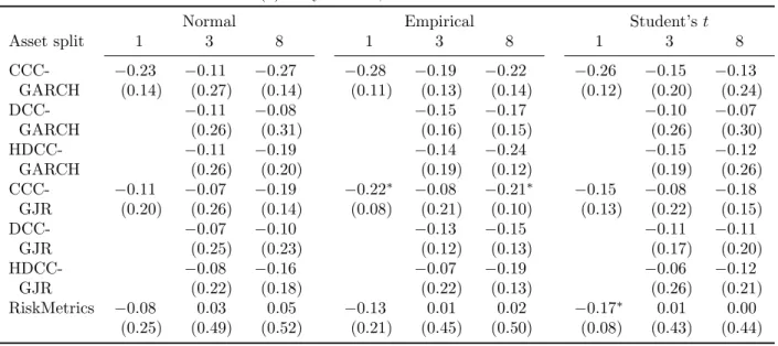
Next, we turn to the dynamic quantile (DQ) test based on Equation (21) to investigate whether the forecast quality varies with the magnitude of the VaR forecast. The summary results are in Table 1, and the full results in Table C.2. Mostly, the relation between a violation and the forecast is not significant, with only 40 rejections out of 255 methods. Nevertheless, the estimates and in particular their signs give useful insights into the forecast quality. A positive sign means that risk is overestimated in times of distress, because a larger than average VaR forecast (a value forqj_t below average) decreases the probability of a violation. Risk is then underestimated for quiet times. For negative signs, the interpretation is reversed.

Temporal aggregation has a clear effect on the forecast quality. The use of daily returns leads to a slight underestimation of risk in times of distress for 46 methods, but to overes-timation for only five. These results indicate that models based on daily returns generally revert a bit too fast to the steady-state volatility. A closer inspection of Table C.20a shows that the five positive coefficients are all for forecasts based on RiskMetrics, where mean-reversion is absent. The negative coefficients are mostly insignificant, but a richer GARCH specification may improve the forecasts. For weekly returns, the number of positive and negative coefficients are about equal. For biweekly returns all coefficients are positive, and 30 out of 51 are significant. Here, mean reversion is clearly too slow.

Full portfolio aggregation leads more often to positive than to negative coefficients (27 versus 18), but this pattern reverses for less aggregation. When all assets are considered, 73 methods lead to negative coefficients and 32 to positive ones. When three basic assets

are used, positive and negative coefficients are more balanced. Also in the cross-sectional dimension, methods with a low degree of aggregation lead more often to an underestimation of VaR in times of distress.

The results for the different model specifications show again the effect of mean reversion. In the univariate case, we find more evidence for overestimation of VaR in times of distress, compared to the multivariate cases. A more precise identification of the nature of the shocks may help, but it is not clear which specification is best, as the differences between the six multivariate GARCH models are quite small. The asymmetry captured by the GJR model has small effects on iterated forecasts (daily or weekly) but leads to underestimation of risk in times of distress when forecasts are scaled. The difference between CCC, DCC and HDCC models is generally larger when eight assets are considered than three. In the CCC models correlations are assumed to be constant, so it leads more often to underestimation. The RiskMetrics model, which does not imply mean reversion, leads to overestimation.

Overall, we conclude that the results of the DQ-test are mostly related to the speed of mean reversion implied by the models. When mean reversion is relatively fast, the DQ-test indicates a slight underestimation of risk in times of distress, though mostly insignificant. This effect is clearest when daily data and/or CCC models are chosen. When mean reversion is slower and shocks become more persistent, the DQ-tests signal overestimation in times of distress. Significance is a bit stronger, though the majority of methods show insignificant coefficients. The differences between the distributions are small. All show about as many positive as negative coefficients. The same conclusion applies to iterating versus scaling.

Summarizing, we find that temporal aggregation has a large impact on the forecast qua-lity. Using weekly or biweekly data leads to too frequent violations, though more often during quiet times. Portfolio aggregation has less impact. Modeling on the level of asset classes gives the best results for coverage and time-variation. The model choice is also of less importance. Differences between the combinations of CCC/DCC/HDCC and GARCH/GJR methods are small, but still indicate a preference for the DCC/HDCC-GJR method. Diffe-rences with RiskMetrics are somewhat larger. The choice for the distribution is again more important. In particular distributions with fat tails lead to better coverage ratios. The fore-casting method is important when daily data are used, with iterated forecasts outperforming scaled ones.

We conclude that more detailed information on shocks as provided by daily data on the asset or asset class level, and a more detailed specification of their propagation in the form of

a richer model and iterated forecasts, improve forecast quality. Increased aggregation means that sometimes shocks are missed, whereas the one-size-fits-all approach of the RiskMetrics methods, and the scaling of forecasts lead to a too strong extrapolation of the effects of shocks. On the other hand, we find that detailed information, models and forecasting increase the risk of forecast errors. So far, the benefits of an increased level of detail outweigh these errors.

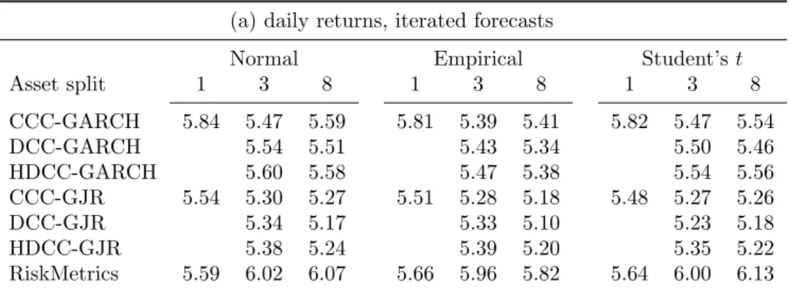
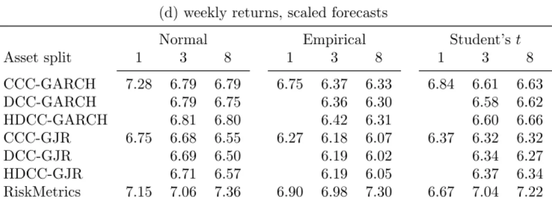
4.1.2 Relative forecast quality

We now turn to a statistical comparison of the different methods. For each method, we calculate the average asymmetric tick loss as in Equation (22), reported in Table 2. The lowest loss (5.10×10−2) is obtained by constructing iterated forecasts based on daily data for eight assets, with a DCC-GJR model and the empirical distribution. The largest loss (8.95×10−2) results from a direct forecast based on biweekly data for eight assets with the RiskMetrics approach and the empirical distribution.

[Table 2 about here.] [Table 2 (continued) about here.]

We construct the Model Confidence Set (MCS) (Hansen et al., 2011) with a significance level of 10% to determine the importance of the different choice aspects. The results in Table 3 show that the observation frequency is the most important choice. None of the methods based on daily observations are removed from the MCS, neither when iterated nor when scaled forecasts are constructed. A lower frequency leads to more removals: 7 for weekly observations combined with iterated forecasts, 13 for the combination with scaled forecasts, and 31 for biweekly observations. So, less temporal aggregation clearly leads to better results.

[Table 3 about here.]

When weekly data are used to construct iterated forecasts, the seven models that are excluded typically do not allow for enough dynamics (Table 3a). Five of the excluded models use RiskMetrics, the other two use a univariate GARCH specification. Along the dimension of portfolio aggregation, five excluded models model at the portfolio level, the other two at the asset class level. The exclusions seem not particularly related to the distributions.

The removals from the subset of scaled forecasts based on weekly data in Table 3b show a slightly clearer pattern. Of the 13 removed methods five use RiskMetrics, and three use CCC-GARCH. The other five are spread over the other model choices. Looking at the portfolio aggregation, seven removals model returns at the portfolio level, five at the asset class level and only one at the asset level. We now see that the Student’s t-distribution counts only two removals, whereas the normal counts six removals, and the empirical five.

From the 51 methods based on biweekly data in Table 3c, 31 are removed and 20 remain. In particular, all 17 models based on the empirical distribution are excluded, compared to five for the normal distribution and nine for the Student’st-distribution. The sample size of 100 observations is too small to reliably construct the empirical distribution, and even gives trouble for the Student’s t-distribution.

From the subset of methods that use either the normal or Student’s t-distribution, all models on the portfolio level are excluded. From the models based on the asset class level, six are removed, compared to only two from the models based on the asset level. With regard to the model specification, the RiskMetrics approach often leads to exclusion (four out of six). We do not observe a clear pattern in the in- or exclusion of the other model specifications.

We conclude that using observations at the asset level, and to a lesser extent at the asset class level, can compensate for the low detail in the temporal dimension. Also, a model specification with richer dynamics can offer some compensation. Working with biweekly data typically leads to larger losses than using data with a higher frequency, whatever the portfolio details or model specification.

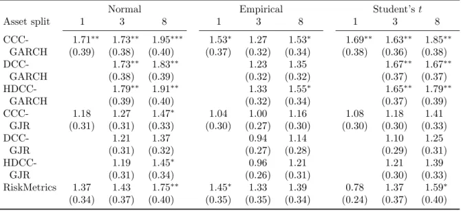
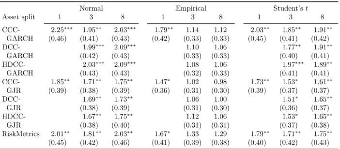
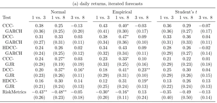
We now investigate whether the methods that use daily data can yield some further insight into the consequences of the remaining choices. The MCS results shows that no particular combination stands out, as all models are included in the MCS. Also when we start the MCS procedure with only the 110 daily methods, no methods are removed from this set. Therefore, we conduct pairwise comparisons of those methods that differ in only one choice aspect based on the Diebold-Mariano test. For example, we test whether the DCC-GJR specification leads to the same average loss as the RiskMetrics specification, when iterated forecasts are constructed based on daily data at the asset level using the empirical distribution. Detailed results are available in Appendix C.1. We summarize them in Table 4.

Our results show a preference for iterated forecasts. For 38 out of 51 comparisons, the losses from iterated forecasts are lower than from scaled forecasting. Six (14) loss differen-tials are significant at the 5% (10%) level. Because of this difference, we separately report summary statistics for iterated and scaled forecasts.

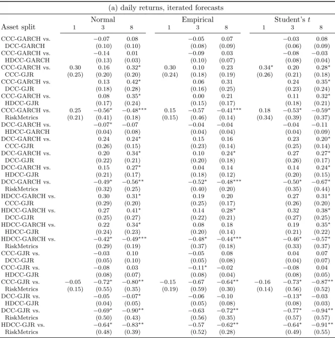
The results for portfolio aggregation (panels b and c) confirm our conclusion from the MCS that a low degree of portfolio aggregation leads to better performance. Modeling at the asset level leads to lower losses for 16 (18) out of 21 methods that use iterated forecasts, when compared to modeling at the asset class (portfolio) level. Modeling at the asset class level beats modeling at the portfolio level also 21 times. However, differences are generally not significant. For scaled forecasts, results are similar. These results are consistent with the preference for multivariate models reported by Santos et al. (2013).

With regard to the distribution choice, the normal distribution loses from the empirical and Student’s t-distributions in 13 (15) out of 17 comparisons based on iterated forecasts, and for all 17 comparisons based on scaled forecasts. The empirical distribution is preferred to the Student’s t-distribution. This result may be due to the skewness that the empirical distribution can capture, and contrasts with the bad results for the empirical distribution when biweekly data are used. The empirical distribution only works well when a large number of observations is available.

The number of comparisons of model specifications is large, because we analyze 7 speci-fications. We therefore summarize our results such that we can see the consequences of the parsimonious specification of RiskMetrics versus the richer (multivariate) GARCH specifi-cations, the asymmetric effects in the marginal specification (GARCH vs. GJR), and the dynamics in the multivariate part (CCC, DCC and HDCC).

Panels f and g clearly show a preference for richer model specifications than RiskMetrics. All 36 multivariate models produce a lower average loss than RiskMetrics, which is significant for 15 (12) methods with iterated (scaled) forecasts. For the univariate case, the results are more mixed. Given the preference for multivariate models in panels b and c, we conclude that allowing for a separate specification of the dynamics in the marginal volatilities and in the dependence is worthwhile.

Our results also show a clear preference for the asymmetric specification of the volatility dynamics in the GJR-GARCH model. When iterated forecasts are used, the univariate GJR specification beats GARCH for 3 out of 3 methods. For the multivariate specifications, it does so for 53 out of 54 methods, with 20 loss differentials that are significant at the 10%

level. When scaled forecasts are used, the evidence is also in favor of the GJR specification, though less pronounced.

We do not find a clear winner for the dynamics in the dependence. The CCC specification leads to losses that are not that different from the DCC/HDCC specifications. The HDCC specification performs less than DCC, in particular when scaled forecasts are constructed.

Summarizing, the DM tests indicate that methods that have more information available and make better use of it lead to lower losses, though differences are often not significant. For portfolio aggregation, we find a preference for models at the asset or asset class level. For the distribution, the empirical one is preferred. Multivariate models with asymmetric effects in the volatility are preferred, but correlation dynamics do not matter much.

4.2

VaR forecasts with a 95% confidence level

We repeat our analyses for VaR forecasts with a confidence level of 95%. We focus here on the main findings, and provide the full set of results in Appendix C.2. In the discussion below, we always use the test outcomes at the 5% significance level, except for the results of the Model Confidence Set, which uses again the 10% significance level.

In terms of absolute forecasting quality, the different methods show better coverage ratios than for the 99% VaR forecasts. Based on their 95% VaR-forecasts, only 49 methods (out of 255) are rejected, compared to 149 based on their 99% VaR forecasts. This drop in the number of rejections is concentrated in the methods that use the normal distribution, as it goes down from 75 to only 11. For the Student’s t-distribution, the number of rejections decreases from 67 to 38, indicating that the normal distribution now leads to better coverage. When we use a significance level of 10%, the empirical distribution outperforms both the normal and Student’s t-distribution with 4 compared to 47 and 61 rejections.

The rejections based on the 95% VaR forecasts are more concentrated in the methods that use biweekly observations (19 out of 51), which further strengthens the preference for less time aggregation. The options for the portfolio aggregation and for the model are more or less equally affected, and show similar drops in the number of rejections.

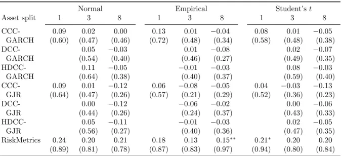
The DQ-tests find more evidence of time variation of the VaR exceedances. Based on the 95% VaR forecasts, 65 coefficients are significantly positive, compared to 35 based on the 99% VaR forecasts. We also find more positive coefficients for the 95% case (198 compared to 117). In particular, the coefficients are positive when weekly and biweekly data are used to construct forecasts. This finding indicates more overestimation of risk in times of distress.

The differences with the 99% case may point at changes in the shape of the distributions, but we do not investigate this issue in more detail.

The average losses can be estimated more precisely based on the 95% VaR forecasts. As a consequence, the MCS becomes smaller: 126 methods are maintained, and 129 are removed. Recall that for the 99% VaR forecasts, only 51 models are removed. The removals are again concentrated in the methods that use a larger degree of temporal aggregation. Many methods that generate forecasts based on weekly data are removed (75 out of 102), and even all that use biweekly data. From the 110 methods that use daily data only 3 are removed.

The pattern that we observe for the removals from the subset of methods that use weekly data for 99% VaR forecasts is stronger for 95% forecasts. All methods that model on the asset class or portfolio level are out, as are all methods that use RiskMetrics, and most methods that use the empirical distribution. The three excluded methods from the subset based on daily data all use RiskMetrics.

The pairwise comparison of the different methods based on daily data also show a stronger preference for no portfolio aggregation. Losses are again lower for models at the asset level, but now the differences are significant for 5 and 13 out of 21 comparisons with models at the asset class and portfolio level.

The method of constructing forecasts and the distribution for innovations are less conse-quential for 95% VaR forecasts. Though losses tend to be lower for scaled forecasts of 95% VaR (42 times compared to 17 times for the 99% VaR), only one differential is significant. Also, the normal distribution does not lead as often to negative losses.

The pairwise comparisons of the different model specifications yields similar results as for 99% VaR forecasts. RiskMetrics loses from richer multivariate GARCH specifications. Within the latter subset, models with the asymmetric GJR specification for the marginal volatility process outperform models with the symmetric specification, and the choice for CCC, DCC or HDCC does not matter much.

We conclude that the degree of time aggregation is the most important choice, both for 99% and 95% VaR forecasts. Using daily data leads to the best coverage and the lowest losses. For 95% VaR forecasts, the degree of portfolio aggregation becomes more important, though it remains less consequential that the degree of temporal aggregation. Models as the asset level lead to reasonable coverage, and to lower losses than models at the asset class or portfolio level. Daily observations at the asset level are best combined with models that

specify the effects of shocks more precisely. The choice for the distribution is important for 99% VaR forecasts, with the empirical and Student’s t-distribution outperforming the normal distribution. For the 95% VaR forecasts, the distribution matters less. The same holds for the forecasting method.

4.3

Longer estimation window

Our main result that methods with daily data outperform those with (bi)weekly data can have two causes. Methods based on daily data can better capture the propagation of shocks, but the better performance can also reflect increased efficiency because more observations are available for estimation. In particular, 100 biweekly observations may be too few to reliably estimate the parameters in multivariate GARCH models. Therefore, we investigate how our results change when we double the estimation window from approximately four to eight years. So, instead of 1,000, 200 and 100 observations, we now use 2,000, 400 and 200 observations for estimation in the daily, weekly and biweekly methods. We discuss the main findings here, and present the detailed results in Appendix C.3. If efficiency is the main driver of our result, we should see an improvement in the forecast quality of methods based on weekly and especially biweekly data, both in absolute sense and in comparison with methods based on daily data.

Regarding absolute forecast quality, we observe only slight improvements for biweekly data. Using the 4-year estimation window, correct unconditional coverage is rejected for 39 out of 51 methods at the 5% significance level (see Table 1). The DQ-test leads to 30 rejections. For the 8-year window, these tests produce 36 and 11 rejections. For weekly data results become a bit worse.

Our analyses of relative forecast quality show smaller differences between all methods when using an 8-year estimation window. The MCS contains all methods based on daily and weekly data, and only six methods based on biweekly data are removed. Pairwise com-parisons with DM-tests show that daily methods with iterated (scaled) forecasts significantly (at 5% level) outperform weekly methods 14 (18) times using a 4-year estimation window. These numbers go down to 8 (11) using a 8-year window. The comparison of daily versus biweekly methods shows a reduction of 34 (26) to 19 (19). However, at the 10% level, results are the same for both windows. Moreover, the loss differentials actually increase for the 8-year window, and so do their standard errors, which explains the decreased significance.

prefera-ble, because it leads to methods that better capture the propagation of shocks. Our results for portfolio aggregation point in the same direction. An increase in the number of modeled assets also leads to models that better capture shocks, without affecting efficiency.

5

Conclusion

In this paper we investigate the importance of the degree of aggregation for forecasting 99% and 95% ten-day ahead Value-at-Risk (VaR). We analyze the effect of aggregating daily returns to weekly and biweekly returns, and aggregation of assets into the main asset classes and into a single portfolio. We compare the importance of aggregation to those of choosing a time-series model (asymmetric or symmetric GARCH, constant or time-varying correlation, or the RiskMetrics approach), choosing a distribution (the Gaussian, Student’s t, or the empirical distribution), and choosing a method for forecast construction (iterated or scaled). Our main finding is that the degree of temporal aggregation is the most important choice. Using daily returns leads to better VaR forecasts than (bi)weekly returns. The dynamics in the distribution of returns is best captured at the daily level. A higher degree of aggregation leads to a loss of important details. The chosen model and distribution also matter for the forecasts. When daily returns are chosen, the model is the second-most important choice. Because the dynamics are present in great detail, the model should accurately capture them. Because weekly or biweekly returns obscure the return dynamics, the chosen distribution becomes more important than the model.

We find that multivariate models outperform univariate ones, confirming Santos et al. (2013), though the differences are not that large, and often not significant. The degree of portfolio aggregation affects forecast quality less than the degree of temporal aggregation, the model and distribution choice. Iterating forecasts are better than scaled and direct forecasts. This holds in particular for the 99% VaR. Scaled forecasts generally perform better than direct forecasts, in line with Ghysels et al. (2009).

We advise to construct models on the asset class level based on daily data. The model had best contain asymmetric effects on the marginal level, but correlation dynamics are not consequential. The distribution should allow for fat tails, in particular for 99% VaR forecasts. It is also best to iterate forecasts. However, applying the RiskMetrics approach with scaling does not make forecasts that much worse.

References

Aielli, G. P. (2013). Dynamic conditional correlation: on properties and estimation. Journal of Business & Economic Statistics, 31(3):282–299.

Andersen, T. G., Bollerslev, T., Christoffersen, P. F., and Diebold, F. X. (2006). Volatility and correlation forecasting. In Elliot, G., Granger, C. W., and Timmermann, A., editors,Handbook of Economic Forecasting, volume 1, chapter 15, pages 777–878. Elsevier North Holland, Amsterdam, Netherlands.

Bao, Y., Lee, T.-H., and Saltoglu, B. (2006). Evaluating predictive performance of value-at-risk models in emerging markets: A reality check. Journal of Forecasting, 25(2):101–128.

Basel Committee on Banking Supervision (1996). Amendment to the capital accord to incorporate market risks. Technical Report Committee Report 24, Basel Committee on Banking Supervision, Basel, Switzerland.

Bauwens, L., Grigoryeva, L., and Ortega, J.-P. (2016). Estimation and empirical performance of non-scalar dynamic conditional correlation models. Computational Statistics & Data Analysis, 100:17–36.