Experiments with MATLAB

Experiments with MATLAB

Cleve Moler

Copyright 2011

Cleve Moler

Electronic edition published by MathWorks, Inc. http://www.mathworks.com/moler

Contents

Preface iii

1 Iteration 1

2 Fibonacci Numbers 17

3 Calendars and Clocks 33

4 Matrices 45 5 Linear Equations 63 6 Fractal Fern 75 7 Google PageRank 83 8 Exponential Function 97 9 T Puzzle 113 10 Magic Squares 123 11 TicTacToe Magic 141 12 Game of Life 151 13 Mandelbrot Set 163 14 Sudoku 183

15 Ordinary Differential Equations 199

16 Predator-Prey Model 213

17 Orbits 221

18 Shallow Water Equations 241

19 Morse Code 247

Experiments with MATLAB

⃝

Cleve Moler

Copyright c⃝2011 Cleve Moler.

All rights reserved. No part of this e-book may be reproduced, stored, or trans-mitted in any manner without the written permission of the author. For more information, [email protected].

The programs described in this e-book have been included for their instructional value. These programs have been tested with care but are not guaranteed for any particular purpose. The author does not offer any warranties or representations, nor does he accept any liabilities with respect to the use of the programs. These programs should not be relied on as the sole basis to solve a problem whose incorrect solution could result in injury to person or property.

Matlab⃝R is a registered trademark of MathWorks, Inc.TM.

For more information about relevant MathWorks policies, see:

http://www.mathworks.com/company/aboutus/policies_statements

Preface

Figure 1. exmgui provides a starting point for some of the experiments.

Welcome toExperiments with MATLAB. This is not a conventional book. It is currently available only via the Internet, at no charge, from

http://www.mathworks.com/moler

There may eventually be a hardcopy edition, but not right away.

Although Matlab is now a full fledged Technical Computing Environment, it started in the late 1970s as a simple “Matrix Laboratory”. We want to build on this laboratory tradition by describing a series of experiments involving applied mathematics, technical computing, and_Matlabprogramming.

We expect that you already know something about high school level material in geometry, algebra, and trigonometry. We will introduce ideas from calculus, matrix theory, and ordinary differential equations, but we do not assume that you have already taken courses in the subjects. In fact, these experiments are useful supplements to such courses.

We also expect that you have some experience with computers, perhaps with word processors or spread sheets. If you know something about programming in languages like C or Java, that will be helpful, but not required. We will introduce

Matlabby way of examples. Many of the experiments involve understanding and

modifyingMatlabscripts and functions that we have already written.

You should have access to Matlab and to our exm toolbox, the collection of programs and data that are described inExperiments with MATLAB. We hope you will not only use these programs, but will read them, understand them, modify them, and improve them. Theexmtoolbox is the apparatus in our “Laboratory”.

You will want to have _Matlab handy. For information about the Student Version, see

http://www.mathworks.com/academia/student_version

For an introduction to the mechanics of using_Matlab, see the videos at http://www.mathworks.com/academia/student_version/start.html For documentation, including “Getting Started”, see

http://www.mathworks.com/access/helpdesk/help/techdoc/matlab.html For user contributed programs, programming contests, and links into the world-wide

Matlabcommunity, check out

http://www.mathworks.com/matlabcentral

To get started, download the exmtoolbox, use pathtool to add exm to the

Matlabpath, and runexmguito generate figure 1. You can click on the icons to preview some of the experiments.

You will want to make frequent use of the_Matlab help and documentation facilities. To quickly learn how to use the command or function namedxxx, enter

help xxx

For more extensive information aboutxxx, use doc xxx

We hope you will find the experiments interesting, and that you will learn how to use_Matlabalong the way. Each chapter concludes with a “Recap” section that is actually an executable_Matlab program. For example, you can review the Magic Squares chapter by entering

Preface v Better yet, enter

edit magic_recap

and run the program cell-by-cell by simultaneously pressing the Ctrl-Shift-Enter keys.

A fairly new_Matlabfacility is thepublishcommand. You can get a nicely formatted web page aboutmagic_recap with

publish magic_recap

If you want to concentrate on learning Matlab, make sure you read, run, and understand the recaps.

Cleve Moler October 4, 2011

Chapter 1

Iteration

Iteration is a key element in much of technical computation. Examples involving the Golden Ratio introduce the _Matlab assignment statement, for andwhile loops, and the plot function.

Start by picking a number, any number. Enter it into_Matlab by typing x =your number

This is a Matlab assignment statement. The number you chose is stored in the variable xfor later use. For example, if you start with

x = 3

Matlabresponds with x =

3

Next, enter this statement x = sqrt(1 + x)

The abbreviation sqrt is the _Matlab name for the square root function. The quantity on the right,√1 +x, is computed and the result stored back in the variable x, overriding the previous value ofx.

Somewhere on your computer keyboard, probably in the lower right corner, you should be able to find four arrow keys. These are thecommand line editingkeys. The up-arrow key allows you to recall earlier commands, including commands from

Copyright c⃝2011 Cleve Moler

Matlab⃝R is a registered trademark of MathWorks, Inc.TM

October 4, 2011

previous sessions, and the other arrows keys allow you to revise these commands. Use the up-arrow key, followed by the enter or return key, to iterate, or repeatedly execute, this statement:

x = sqrt(1 + x)

Here is what you get when you start withx = 3. x = 3 x = 2 x = 1.7321 x = 1.6529 x = 1.6288 x = 1.6213 x = 1.6191 x = 1.6184 x = 1.6181 x = 1.6181 x = 1.6180 x = 1.6180

These values are 3, √1 + 3, √1 +√1 + 3,

√

1 +√1 +√1 + 3, and so on. After 10 steps, the value printed remains constant at1.6180. Try several other starting values. Try it on a calculator if you have one. You should find that no matter where you start, you will always reach1.6180in about ten steps. (Maybe a few more will be required if you have a very large starting value.)

Matlabis doing these computations to accuracy of about 16 decimal digits,

but is displaying only five. You can see more digits by first entering format long

and repeating the experiment. Here are the beginning and end of 30 steps starting atx= 3.

x = 3

3 x = 2 x = 1.732050807568877 x = 1.652891650281070 .... x = 1.618033988749897 x = 1.618033988749895 x = 1.618033988749895

After about thirty or so steps, the value that is printed doesn’t change any more. You have computed one of the most famous numbers in mathematics, ϕ, the Golden Ratio.

In Matlab, and most other programming languages, the equals sign is the assignment operator. It says compute the value on the right and store it in the variable on the left. So, the statement

x = sqrt(1 + x)

takes the current value ofx, computessqrt(1 + x), and stores the result back in x.

In mathematics, the equals sign has a different meaning. x=√1 +x

is anequation. A solution to such an equation is known as afixed point. (Be careful not to confuse the mathematical usage offixed point with the computer arithmetic usage offixed point.)

The function f(x) = √1 +x has exactly one fixed point. The best way to find the value of the fixed point is to avoid computers all together and solve the equation using the quadratic formula. Take a look at the hand calculation shown in figure 1.1. The positive root of the quadratic equation is the Golden Ratio.

ϕ= 1 +

√

5 2 .

You can haveMatlab computeϕdirectly using the statement phi = (1 + sqrt(5))/2

Withformat long, this produces the same value we obtained with the fixed point iteration,

phi =

Figure 1.1. Compute the fixed point by hand. −1 0 1 2 3 4 −1 −0.5 0 0.5 1 1.5 2 2.5 3 3.5 4

Figure 1.2. A fixed point at ϕ= 1.6180.

Figure 1.2 is our first example of Matlabgraphics. It shows the intersection of the graphs ofy=xandy=√1 +x. The statement

x = -1:.02:4;

generates a vector x containing the numbers from -1 to 4 in steps of .02. The statements

y1 = x;

y2 = sqrt(1+x);

5 produce a figure that has three components. The first two components are graphs ofxand√1 +x. The’-’argument tells theplotfunction to draw solid lines. The last component in the plot is a single point with both coordinates equal toϕ. The ’o’tells theplotfunction to draw a circle.

The_Matlab plot function has many variations, including specifying other colors and line types. You can see some of the possibilities with

help plot

φ

φ

− 1

1

1

Figure 1.3. The golden rectangle.

The Golden Ratio shows up in many places in mathematics; we’ll see several in this book. The Golden Ratio gets its name from the golden rectangle, shown in figure 1.3. The golden rectangle has the property that removing a square leaves a smaller rectangle with the same shape. Equating the aspect ratios of the rectangles gives a defining equation forϕ:

1 ϕ =

ϕ−1 1 .

Multiplying both sides of this equation byϕproduces the same quadratic polynomial equation that we obtained from our fixed point iteration.

ϕ2−ϕ−1 = 0.

The up-arrow key is a convenient way to repeatedly execute a single statement, or several statements, separated by commas or semicolons, on a single line. Two more powerful constructs are theforloop and thewhileloop. Aforloop executes a block of code a prescribed number of times.

x = 3

for k = 1:31 x = sqrt(1 + x) end

produces 32 lines of output, one from the initial statement and one more each time through the loop.

Awhileloop executes a block of code an unknown number of times. Termi-nation is controlled by a logical expression, which evaluates totrueorfalse. Here is the simplestwhileloop for our fixed point iteration.

x = 3

while x ~= sqrt(1+x) x = sqrt(1+x) end

This produces the same 32 lines of output as theforloop. However, this code is open to criticism for two reasons. The first possible criticism involves the termi-nation condition. The expressionx ~= sqrt(1+x) is the _Matlab way of writing x̸=√1 +x. With exact arithmetic,xwould never be exactly equal tosqrt(1+x), the condition would always be true, and the loop would run forever. However, like most technical computing environments, _Matlab does not do arithmetic exactly. In order to economize on both computer time and computer memory,_Matlabuses floating point arithmetic. Eventually our program produces a value ofxfor which the floating point numbersxandsqrt(1+x)are exactly equal and the loop termi-nates. Expecting exact equality of two floating point numbers is a delicate matter. It works OK in this particular situation, but may not work with more complicated computations.

The second possible criticism of our simplewhileloop is that it is inefficient. It evaluatessqrt(1+x)twice each time through the loop. Here is a more complicated version of thewhileloop that avoids both criticisms.

x = 3 y = 0;

while abs(x-y) > eps(x) y = x;

x = sqrt(1+x) end

The semicolons at the ends of the assignment statements involvingyindicate that no printed output should result. The quantityeps(x), is the spacing of the floating point numbers near x. Mathematically, the Greek letter ϵ, or epsilon, often rep-resents a “small” quantity. This version of the loop requires only one square root calculation per iteration, but that is overshadowed by the added complexity of the code. Bothwhileloops require about the same execution time. In this situation, I prefer the firstwhileloop because it is easier to read and understand.

Help and Doc

Matlabhas extensive on-line documentation. Statements like

help sqrt help for

7 provide brief descriptions of commands and functions. Statements like

doc sqrt doc for

provide more extensive documentation in a separate window.

One obscure, but very important,helpentry is about the various punctuation marks and special characters used by_Matlab. Take a look now at

help punct doc punct

You will probably want to return to this information as you learn more about

Matlab.

Numbers

Numbers are formed from the digits 0 through 9, an optional decimal point, a leading +or -sign, an optionale followed by an integer for a power of 10 scaling, and an optionaliorjfor the imaginary part of a complex number. _Matlabalso knows the value ofπ. Here are some examples of numbers.

42

9.6397238 6.0221415e23 -3+4i

pi

Assignment statements and names

A simple assignment statement consists of a name, an = sign, and a number. The names of variables, functions and commands are formed by a letter, followed by any number of upper and lower case letters, digits and underscores. Single character names, like xand N, and anglicized Greek letters, likepi andphi, are often used to reflect underlying mathematical notation. Non-mathematical programs usually employ long variable names. Underscores and a convention known as camel casing are used to create variable names out of several words.

x = 42

phi = (1+sqrt(5))/2

Avogadros_constant = 6.0221415e23 camelCaseComplexNumber = -3+4i

Expressions

Power is denoted by ^ and has precedence over all other arithmetic operations. Multiplication and division are denoted by *, /, and \ and have precedence over addition and subtraction, Addition and subtraction are denoted by + and - and

have lowest precedence. Operations with equal precedence are evaluated left to right. Parentheses delineate subexpressions that are evaluated first. Blanks help readability, but have no effect on precedence.

All of the following expressions have the same value. If you don’t already recognize this value, you can ask Google about its importance in popular culture.

3*4 + 5*6 3 * 4+5 * 6 2*(3 + 4)*3 -2^4 + 10*29/5 3\126 52-8-2

Recap

%% Iteration Chapter Recap

% This is an executable program that illustrates the statements % introduced in the Iteration chapter of "Experiments in MATLAB". % You can run it by entering the command

%

% iteration_recap %

% Better yet, enter %

% edit iteration_recap %

% and run the program cell-by-cell by simultaneously % pressing the Ctrl-Shift-Enter keys.

% % Enter %

% publish iteration_recap %

% to see a formatted report. %% Help and Documentation % help punct % doc punct %% Format format short 100/81 format long 100/81 format short

9

format compact

%% Names and assignment statements x = 42 phi = (1+sqrt(5))/2 Avogadros_constant = 6.0221415e23 camelCaseComplexNumber = -3+4i %% Expressions 3*4 + 5*6 3 * 4+5 * 6 2*(3 + 4)*3 -2^4 + 10*29/5 3\126 52-8-2 %% Iteration

% Use the up-arrow key to repeatedly execute x = sqrt(1+x) x = sqrt(1+x) x = sqrt(1+x) x = sqrt(1+x) %% For loop x = 42 for k = 1:12 x = sqrt(1+x); disp(x) end %% While loop x = 42; k = 1;

while abs(x-sqrt(1+x)) > 5e-5 x = sqrt(1+x);

k = k+1; end

k

%% Vector and colon operator k = 1:12

x = (0.0: 0.1: 1.00)’ %% Plot

x = -pi: pi/256: pi;

z = 1 + tan(1); plot(x,y,’-’, pi/2,z,’ro’) xlabel(’x’) ylabel(’y’) title(’tan(sin(x)) - sin(tan(x))’) %% Golden Spiral golden_spiral(4)

Exercises

1.1Expressions. Use_Matlabto evaluate each of these mathematical expressions. 432 −34 _{sin 1} 4(32₎ (−3)4 _{sin 1}◦ (43₎2 √4−_{3 sin}π 3 4 √ 32 −2−4/3 _{(arcsin 1)/π}

You can get started with help ^

help sin

1.2Temperature conversion.

(a) Write a_Matlabstatement that converts temperature in Fahrenheit,f, to Cel-sius,c.

c =something involving f

(b) Write a_Matlabstatement that converts temperature in Celsius,c, to Fahren-heit,f.

f =something involving c

1.3Barn-megaparsec. Abarn is a unit of area employed by high energy physicists. Nuclear scattering experiments try to “hit the side of a barn”. Aparsec is a unit of length employed by astronomers. A star at a distance of one parsec exhibits a trigonometric parallax of one arcsecond as the Earth orbits the Sun. A barn-megaparsecis therefore a unit of volume – a very long skinny volume.

A barn is 10−28 square meters. A megaparsec is 106 parsecs. A parsec is 3.262 light-years. A light-year is 9.461·1015 _meters.

A cubic meter is 106_milliliters.

A milliliter is 1

11 Express one barn-megaparsec in teaspoons. In _Matlab, the letter e can be used to denote a power of 10 exponent, so 9.461·1015 _{can be written9.461e15.}

1.4Complex numbers. What happens if you start with a large negative value ofx and repeatedly iterate

x = sqrt(1 + x)

1.5Comparison. Which is larger,πϕ _{or ϕ}π_? 1.6Solving equations. The best way to solve

x=√1 +x or

x2= 1 +x

is to avoid computers all together and just do it yourself by hand. But, of course,

Matlaband most other mathematical software systems can easily solve such equa-tions. Here are several possible ways to do it withMatlab. Start with

format long

phi = (1 + sqrt(5))/2

Then, for each method, explain what is going on and how the resulting x differs fromphiand the otherx’s.

% roots help roots x1 = roots([1 -1 -1]) % fsolve help fsolve f = @(x) x-sqrt(1+x) p = @(x) x^2-x-1 x2 = fsolve(f, 1) x3 = fsolve(f, -1) x4 = fsolve(p, 1) x5 = fsolve(p, -1)

% solve (requires Symbolic Toolbox or Student Version) help solve

help syms syms x

x6 = solve(’x-sqrt(1+x)=0’) x7 = solve(x^2-x-1)

1.7Symbolic solution. If you have the Symbolic Toolbox or Student Version, explain what the following program does.

x = sym(’x’) length(char(x)) for k = 1:10 x = sqrt(1+x) length(char(x)) end

1.8Fixed points. Verify that the Golden Ratio is a fixed point of each of the following equations.

ϕ= 1 ϕ−1 ϕ= 1

ϕ+ 1

Use each of the equations as the basis for a fixed point iteration to computeϕ. Do the iterations converge?

1.9 Another iteration. Before you run the following program, predict what it will do. Then run it.

x = 3 k = 1 format long while x ~= sqrt(1+x^2) x = sqrt(1+x^2) k = k+1 end

1.10Another fixed point. Solve this equation by hand. x=√ 1

1 +x2

How many iterations does the following program require? How is the final value of xrelated to the Golden Ratio ϕ?

x = 3 k = 1 format long while x ~= 1/sqrt(1+x^2) x = 1/sqrt(1+x^2) k = k+1 end

13 1.11cos(x). Find the numerical solution of the equation

x= cosx

in the interval [0,π₂], shown in figure 1.4.

0 0.5 1 1.5 0

0.5 1 1.5

Figure 1.4. Fixed point of x = cos(x).

−6 −4 −2 0 2 4 6 −6 −4 −2 0 2 4 6

Figure 1.5. Three fixed points of x = tan(x)

1.12tan(x). Figure 1.5 shows three of the many solutions to the equation x= tanx

One of the solutions is x = 0. The other two in the plot are near x = ±4.5. If we did a plot over a large range, we would see solutions in each of the intervals [(n−1₂)π,(n+1₂)π] for integern.

(a) Does this compute a fixed point? x = 4.5

for k = 1:30 x = tan(x) end

(b) Does this compute a fixed point? Why is the “ + pi” necessary? x = pi

while abs(x - tan(x)) > eps(x) x = atan(x) + pi

end

1.13Summation. Write a mathematical expression for the quantity approximated by this program. s = 0; t = Inf; n = 0; while s ~= t n = n+1; t = s; s = s + 1/n^4; end s

1.14Why. The first version ofMatlab written in the late 1970’s, hadwho,what, which, andwherecommands. So it seemed natural to add awhycommand. Check out today’swhycommand with

why help why

for k = 1:40, why, end type why

edit why

As thehelp entry says, please embellish or modify thewhy function to suit your own tastes.

1.15Wiggles. A glimpse at_Matlabplotting capabilities is provided by the function f = @(x) tan(sin(x)) - sin(tan(x))

This uses the ’@’ sign to introduce a simple function. You can learn more about the ’@’ sign withhelp function_handle.

Figure 1.6 shows the output from the statement ezplot(f,[-pi,pi])

15 −3 −2 −1 0 1 2 3 −2.5 −2 −1.5 −1 −0.5 0 0.5 1 1.5 2 2.5 x tan(sin(x))−sin(tan(x))

Figure 1.6. A wiggly function.

(The function name ezplot is intended to be pronounced “Easy Plot”. This pun doesn’t work if you learned to pronounce “z” as “zed”.) You can see that the function is very flat near x = 0, oscillates infinitely often near x = ±π/2 and is nearly linear nearx=±π.

You can get more control over the plot with code like this. x = -pi:pi/256:pi;

y = f(x); plot(x,y) xlabel(’x’) ylabel(’y’)

title(’A wiggly function’) axis([-pi pi -2.8 2.8])

set(gca,’xtick’,pi*(-3:1/2:3))

(a) What is the effect of various values ofnin the following code? x = pi*(-2:1/n:2);

comet(x,f(x))

(b) This function is bounded. A numeric value near its maximum can be found with

max(y)

What is its analytic maximum? (To be precise, I should ask ”What is the function’s supremum?”)

1.16Graphics. We use a lot of computer graphics in this book, but studying

script that produces figure 1.3 is goldrect.m. Modify this program to produce a graphic that compares the Golden Rectangle with TV screens having aspect ratios 4:3 and 16:9.

1.17Golden Spiral

Figure 1.7. A spiral formed from golden rectangles and inscribed quarter circles.

Our programgolden_spiral displays an ever-expanding sequence of golden rectangles with inscribed quarter circles. Check it out.

Chapter 2

Fibonacci Numbers

Fibonacci numbers introduce vectors, functions and recursion.

Leonardo Pisano Fibonacci was born around 1170 and died around 1250 in Pisa in what is now Italy. He traveled extensively in Europe and Northern Africa. He wrote several mathematical texts that, among other things, introduced Europe to the Hindu-Arabic notation for numbers. Even though his books had to be tran-scribed by hand, they were widely circulated. In his best known book,Liber Abaci, published in 1202, he posed the following problem:

A man puts a pair of rabbits in a place surrounded on all sides by a wall. How many pairs of rabbits can be produced from that pair in a year if it is supposed that every month each pair begets a new pair which from the second month on becomes productive?

Today the solution to this problem is known as the Fibonacci sequence, or Fibonacci numbers. There is a small mathematical industry based on Fibonacci numbers. A search of the Internet for “Fibonacci” will find dozens of Web sites and hundreds of pages of material. There is even a Fibonacci Association that publishes a scholarly journal, theFibonacci Quarterly.

A simulation of Fibonacci’s problem is provided by ourexmprogramrabbits. Just execute the command

rabbits

and click on the pushbuttons that show up. You will see something like figure 2.1. If Fibonacci had not specified a month for the newborn pair to mature, he would not have a sequence named after him. The number of pairs would simply

Copyright c⃝2011 Cleve Moler

Matlab⃝R is a registered trademark of MathWorks, Inc.TM

October 4, 2011

Figure 2.1. Fibonacci’s rabbits.

double each month. Aftern months there would be 2n _{pairs of rabbits. That’s a} lot of rabbits, but not distinctive mathematics.

Letfn denote the number of pairs of rabbits afternmonths. The key fact is that the number of rabbits at the end of a month is the number at the beginning of the month plus the number of births produced by the mature pairs:

fn =fn₋1+fn₋2.

The initial conditions are that in the first month there is one pair of rabbits and in the second there are two pairs:

f1= 1, f2= 2.

The following_Matlabfunction, stored in a filefibonacci.mwith a.msuffix, produces a vector containing the firstnFibonacci numbers.

function f = fibonacci(n) % FIBONACCI Fibonacci sequence

19 f = zeros(n,1); f(1) = 1; f(2) = 2; for k = 3:n f(k) = f(k-1) + f(k-2); end

With these initial conditions, the answer to Fibonacci’s original question about the size of the rabbit population after one year is given by

fibonacci(12) This produces 1 2 3 5 8 13 21 34 55 89 144 233

The answer is 233 pairs of rabbits. (It would be 4096 pairs if the number doubled every month for 12 months.)

Let’s look carefully atfibonacci.m. It’s a good example of how to create a

Matlabfunction. The first line is

function f = fibonacci(n)

The first word on the first line saysfibonacci.m is afunction, not a script. The remainder of the first line says this particular function produces one output result, f, and takes one input argument,n. The name of the function specified on the first line is not actually used, becauseMatlablooks for the name of the file with a.m suffix that contains the function, but it is common practice to have the two match. The next two lines are comments that provide the text displayed when you ask for help.

help fibonacci produces

FIBONACCI Fibonacci sequence

The name of the function is in uppercase because historically _Matlab was case insensitive and ran on terminals with only a single font. The use of capital letters may be confusing to some first-time_Matlabusers, but the convention persists. It is important to repeat the input and output arguments in these comments because the first line is not displayed when you ask forhelpon the function.

The next line f = zeros(n,1);

creates an n-by-1 matrix containing all zeros and assigns it to f. In Matlab, a matrix with only one column is a column vector and a matrix with only one row is a row vector.

The next two lines, f(1) = 1;

f(2) = 2;

provide the initial conditions.

The last three lines are theforstatement that does all the work. for k = 3:n

f(k) = f(k-1) + f(k-2); end

We like to use three spaces to indent the body offorandifstatements, but other people prefer two or four spaces, or a tab. You can also put the entire construction on one line if you provide a comma after the first clause.

This particular function looks a lot like functions in other programming lan-guages. It produces a vector, but it does not use any of the _Matlab vector or matrix operations. We will see some of these operations soon.

Here is another Fibonacci function, fibnum.m. Its output is simply the nth Fibonacci number.

function f = fibnum(n) % FIBNUM Fibonacci number.

% FIBNUM(n) generates the nth Fibonacci number. if n <= 1 f = 1; else f = fibnum(n-1) + fibnum(n-2); end The statement fibnum(12) produces ans = 233

21 Thefibnum function isrecursive. In fact, the term recursive is used in both a mathematical and a computer science sense. In mathematics, the relationship fn =fn−1+fn−2 is arecursion relationIn computer science, a function that calls

itself is arecursive function.

A recursive program is elegant, but expensive. You can measure execution time withticandtoc. Try

tic, fibnum(24), toc Donottry

tic, fibnum(50), toc

Fibonacci Meets Golden Ratio

The Golden Ratioϕcan be expressed as an infinite continued fraction. ϕ= 1 + 1

1 + 1

1+ 1

1+··· .

To verify this claim, suppose we did not know the value of this fraction. Let x= 1 + 1

1 + ₁₊11 1+···

.

We can see the first denominator is just another copy ofx. In other words. x= 1 + 1

x

This immediately leads to x2−x−1 = 0

which is the defining quadratic equation forϕ,

Ourexmfunctiongoldfractgenerates aMatlab string that represents the first n terms of the Golden Ratio continued fraction. Here is the first section of code ingoldfract. p = ’1’; for k = 2:n p = [’1 + 1/(’ p ’)’]; end display(p)

We start with a single ’1’, which corresponds ton = 1. We then repeatedly make the current string the denominator in a longer string.

Here is the output fromgoldfract(n)whenn = 7. 1 + 1/(1 + 1/(1 + 1/(1 + 1/(1 + 1/(1 + 1/(1))))))

You can see that there aren-1plus signs andn-1pairs of matching parentheses. Letϕndenote the continued fraction truncated afternterms. ϕn is a rational approximation to ϕ. Let’s express ϕn as a conventional fracton, the ratio of two integers ϕn= pn qn p = 1; q = 0; for k = 2:n t = p; p = p + q; q = t; end

Now compare the results produced bygoldfract(7)andfibonacci(7). The first contains the fraction 21/13 while the second ends with 13 and 21. This is not just a coincidence. The continued fraction for the Golden Ratio is collapsed by repeating the statement

p = p + q;

while the Fibonacci numbers are generated by f(k) = f(k-1) + f(k-2);

In fact, if we letϕndenote the golden ratio continued fraction truncated atnterms, then

ϕn= fn fn₋1

In the infinite limit, the ratio of successive Fibonacci numbers approaches the golden ratio: lim n→∞ fn fn−1 =ϕ.

To see this, compute 40 Fibonacci numbers. n = 40;

f = fibonacci(n); Then compute their ratios.

r = f(2:n)./f(1:n-1)

This takes the vector containing f(2) through f(n) and divides it, element by element, by the vector containingf(1)throughf(n-1). The output begins with

23 2.00000000000000 1.50000000000000 1.66666666666667 1.60000000000000 1.62500000000000 1.61538461538462 1.61904761904762 1.61764705882353 1.61818181818182 and ends with

1.61803398874990 1.61803398874989 1.61803398874990 1.61803398874989 1.61803398874989

Do you see why we chosen = 40? Compute phi = (1+sqrt(5))/2

r - phi

What is the value of the last element?

The first few of these ratios can also be used to illustrate the rational output format. format rat r(1:10) ans = 2 3/2 5/3 8/5 13/8 21/13 34/21 55/34 89/55

The population of Fibonacci’s rabbit pen doesn’t double every month; it is multiplied by the golden ratio every month.

An Analytic Expression

It is possible to find a closed-form solution to the Fibonacci number recurrence relation. The key is to look for solutions of the form

for some constantsc andρ. The recurrence relation fn =fn₋1+fn₋2

becomes

cρn =cρn−1+cρn−2

Dividing both sides bycρn−2 _gives

ρ2=ρ+ 1.

We’ve seen this equation in the chapter on the Golden Ratio. There are two possible values ofρ, namelyϕand 1−ϕ. The general solution to the recurrence is

fn =c1ϕn+c2(1−ϕ)n.

The constantsc1 andc2 are determined by initial conditions, which are now

conveniently written f0 = c1+c2= 1,

f1 = c1ϕ+c2(1−ϕ) = 1.

One of the exercises asks you to use theMatlab backslash operator to solve this 2-by-2 system of simultaneous linear equations, but it is may be easier to solve the system by hand: c1 = ϕ 2ϕ−1, c2 = − (1−ϕ) 2ϕ−1.

Inserting these in the general solution gives fn = 1

2ϕ−1(ϕ

n+1_−(1−ϕ)n+1_).

This is an amazing equation. The right-hand side involves powers and quo-tients of irrational numbers, but the result is a sequence of integers. You can check this with_Matlab.

n = (1:40)’;

f = (phi.^(n+1) - (1-phi).^(n+1))/(2*phi-1) f = round(f)

The.^ operator is an element-by-element power operator. It is not necessary to use./for the final division because(2*phi-1)is a scalar quantity. Roundoff error prevents the results from being exact integers, so the round function is used to convert floating point quantities to nearest integers. The resultingfbegins with

f =

25 2 3 5 8 13 21 34 and ends with

5702887 9227465 14930352 24157817 39088169 63245986 102334155 165580141

Recap

%% Fibonacci Chapter Recap

% This is an executable program that illustrates the statements % introduced in the Fibonacci Chapter of "Experiments in MATLAB". % You can access it with

%

% fibonacci_recap % edit fibonacci_recap % publish fibonacci_recap %% Related EXM Programs % % fibonacci.m % fibnum.m % rabbits.m %% Functions % Save in file sqrt1px.m % % function y = sqrt1px(x) % % SQRT1PX Sample function. % % Usage: y = sqrt1px(x) % % y = sqrt(1+x); %% Create vector n = 8;

f = zeros(1,n) t = 1:n s = [1 2 3 5 8 13 21 34] %% Subscripts f(1) = 1; f(2) = 2; for k = 3:n f(k) = f(k-1) + f(k-2); end f %% Recursion % function f = fibnum(n) % if n <= 1 % f = 1; % else % f = fibnum(n-1) + fibnum(n-2); % end

%% Tic and Toc format short tic

fibnum(24); toc

%% Element-by-element array operations f = fibonacci(5)’ fpf = f+f ftf = f.*f ff = f.^2 ffdf = ff./f cosfpi = cos(f*pi) even = (mod(f,2) == 0) format rat r = f(2:5)./f(1:4) %% Strings hello_world

27

Exercises

2.1 Rabbits. Explain what our rabbits simulation demonstrates. What do the different figures and colors on the pushbuttons signify?

2.2Waltz. Which Fibonacci numbers are even? Why?

2.3 Primes. Use the Matlab function isprime to discover which of the first 40 Fibonacci numbers are prime. You do not need to use a forloop. Instead, check out

help isprime help logical

2.4 Backslash. Use the _Matlab backslashoperator to solve the 2-by-2 system of simultaneous linear equations

c1+c2 = 1,

c1ϕ+c2(1−ϕ) = 1

forc1 and c2. You can find out about the backslash operator by taking a peek at

the Linear Equations chapter, or with the commands help \

help slash

2.5Logarithmic plot. The statement semilogy(fibonacci(18),’-o’)

makes a logarithmic plot of Fibonacci numbers versus their index. The graph is close to a straight line. What is the slope of this line?

2.6 Execution time. How does the execution time of fibnum(n) depend on the execution time forfibnum(n-1)andfibnum(n-2)? Use this relationship to obtain an approximate formula for the execution time of fibnum(n) as a function of n. Estimate how long it would take your computer to computefibnum(50). Warning: You probably do not want to actually runfibnum(50).

2.7Overflow. What is the index of the largest Fibonacci number that can be rep-resented exactly as a _Matlab double-precision quantity without roundoff error? What is the index of the largest Fibonacci number that can be represented approx-imatelyas a_Matlabdouble-precision quantity without overflowing?

The sequence would be defined by g1 = 1, g2 = 1, g3 = 2 and, forn >3, gn =gn−1+gn−3

(a) Modifyfibonacci.m andfibnum.mto compute this sequence. (b) How many pairs of rabbits are there after 12 months?

(c)gn≈γn. What isγ?

(d) Estimate how long it would take your computer to computefibnum(50) with this modifiedfibnum.

2.9Mortality. What if rabbits took one month to mature, but then died after six months. The sequence would be defined by

dn = 0, n <= 0 d1 = 1,

d2 = 1

and, forn >2,

dn=dn₋1+dn₋2−dn₋7

(a) Modifyfibonacci.m andfibnum.mto compute this sequence. (b) How many pairs of rabbits are there after 12 months?

(c)dn≈δn. What isδ?

(d) Estimate how long it would take your computer to computefibnum(50) with this modifiedfibnum.

2.10 Hello World. Programming languages are traditionally introduced by the phrase ”hello world”. An script inexmthat illustrates some features inMatlabis available with

hello_world

Explain what each of the functions and commands inhello_worlddo.

2.11Fibonacci power series. The Fibonacci numbers,fn, can be used as coefficients in a power series defining a function ofx.

F(x) = ∞ ∑ n=1 fnxn = x+ 2x2+ 3x3+ 5x4+ 8x5+ 13x6+...

29 Our functionfibfun1is a first attempt at a program to compute this series. It sim-ply involves adding an accumulating sum tofibonacci.m. The header offibfun1.m includes the help entries.

function [y,k] = fibfun1(x)

% FIBFUN1 Power series with Fibonacci coefficients. % y = fibfun1(x) = sum(f(k)*x.^k).

% [y,k] = fibfun1(x) also gives the number of terms required. The first section of code initializes the variables to be used. The value ofn is the index where the Fibonacci numbers overflow.

\excise

\emph{Fibonacci power series}.

The Fibonacci numbers, $f_n$, can be used as coefficients in a power series defining a function of $x$.

\begin{eqnarray*}

F(x) & = & \sum_{n = 1}^\infty f_n x^n \\

& = & x + 2 x^2 + 3 x^3 + 5 x^4 + 8 x^5 + 13 x^6 + ... \end{eqnarray*}

Our function #fibfun1# is a first attempt at a program to compute this series. It simply involves adding an accumulating sum to #fibonacci.m#.

The header of #fibfun1.m# includes the help entries. \begin{verbatim}

function [y,k] = fibfun1(x)

% FIBFUN1 Power series with Fibonacci coefficients. % y = fibfun1(x) = sum(f(k)*x.^k).

% [y,k] = fibfun1(x) also gives the number of terms required. The first section of code initializes the variables to be used. The value ofn is the index where the Fibonacci numbers overflow.

n = 1476; f = zeros(n,1); f(1) = 1; f(2) = 2; y = f(1)*x + f(2)*x.^2; t = 0;

The main body offibfun1implements the Fibonacci recurrence and includes a test for early termination of the loop.

for k = 3:n f(k) = f(k-1) + f(k-2); y = y + f(k)*x.^k; if y == t return end

t = y; end

There are several objections to fibfun1. The coefficient array of size 1476 is not actually necessary. The repeated computation of powers, x^k, is inefficient because once some power ofxhas been computed, the next power can be obtained with one multiplication. When the series converges the coefficients f(k) increase in size, but the powers x^k decrease in size more rapidly. The terms f(k)*x^k approach zero, but hugef(k)prevent their computation.

A more efficient and accurate approach involves combining the computation of the Fibonacci recurrence and the powers ofx. Let

pk=fkxk Then, since

fk+1xk+1=fkxk+fk₋1xk−1

the termspk satisfy

pk+1 = pkx+pk₋1x2

= x(pk+xpk−1)

This is the basis for our functionfibfun2. The header is essentially the same asfibfun1

function [yk,k] = fibfun2(x)

% FIBFUN2 Power series with Fibonacci coefficients. % y = fibfun2(x) = sum(f(k)*x.^k).

% [y,k] = fibfun2(x) also gives the number of terms required. The initialization. pkm1 = x; pk = 2*x.^2; ykm1 = x; yk = 2*x.^2 + x; k = 0;

And the core.

while any(abs(yk-ykm1) > 2*eps(yk)) pkp1 = x.*(pk + x.*pkm1); pkm1 = pk; pk = pkp1; ykm1 = yk; yk = yk + pk; k = k+1; end

31 There is no array of coefficients. Only three of the pk terms are required for each step. The power function^ is not necessary. Computation of the powers is incor-porated in the recurrence. Consequently,fibfun2is both more efficient and more accurate thanfibfun1.

But there is an even better way to evaluate this particular series. It is possible to find a analytic expression for the infinite sum.

F(x) = ∞ ∑ n=1 fnxn = x+ 2x2+ 3x3+ 5x4+ 8x5+... = x+ (1 + 1)x2+ (2 + 1)x3+ (3 + 2)x4+ (5 + 3)x5+... = x+x2+x(x+ 2x2+ 3x3+ 5x4+...) +x2(x+ 2x2+ 3x3+...) = x+x2+xF(x) +x2F(x) So (1−x−x2)F(x) =x+x2 Finally F(x) = x+x 2 1−x−x2

It is not even necessary to have a.mfile. A one-liner does the job. fibfun3 = @(x) (x + x.^2)./(1 - x - x.^2)

Chapter 3

Calendars and Clocks

Computations involving time, dates, biorhythms and Easter.

Calendars are interesting mathematical objects. The Gregorian calendar was first proposed in 1582. It has been gradually adopted by various countries and churches over the four centuries since then. The British Empire, including the colonies in North America, adopted it in 1752. Turkey did not adopt it until 1923. The Gregorian calendar is now the most widely used calendar in the world, but by no means the only one.

In the Gregorian calendar, a yearyis aleap yearif and only ifyis divisible by 4 and not divisible by 100, or is divisible by 400. InMatlabthe following expression must betrue. The double ampersands, ’&&’, mean “and” and the double vertical bars, ’||’, mean “or”.

mod(y,4) == 0 && mod(y,100) ~= 0 || mod(y,400) == 0

For example, 2000 was a leap year, but 2100 will not be a leap year. This rule implies that the Gregorian calendar repeats itself every 400 years. In that 400-year period, there are 97 leap years, 4800 months, 20871 weeks, and 146097 days. The average number of days in a Gregorian calendar year is 365 +₄₀₀97 = 365.2425.

The_Matlabfunctionclock returns a six-element vectorcwith elements c(1) = year c(2) = month c(3) = day c(4) = hour c(5) = minute c(6) = seconds

Copyright c⃝2011 Cleve Moler

Matlab⃝R is a registered trademark of MathWorks, Inc.TM

October 4, 2011

The first five elements are integers, while the sixth element has a fractional part that is accurate to milliseconds. The best way to print aclockvector is to usefprintf orsprintfwith a specifiedformat string that has both integer and floating point fields.

f = ’%6d %6d %6d %6d %6d %9.3f\n’

I am revising this chapter on August 2, 2011, at a few minutes after 2:00pm, so c = clock; fprintf(f,c); produces 2011 8 2 14 2 19.470 In other words, year = 2011 month = 8 day = 2 hour = 14 minute = 2 seconds = 19.470

The_Matlab functionsdatenum,datevec,datestr, and weekdayuseclock and facts about the Gregorian calendar to facilitate computations involving calendar dates. Dates are represented by theirserial date number, which is the number of days since the theoretical time and day over 20 centuries ago when clock would have been six zeros. We can’t pin that down to an actual date because different calendars would have been in use at that time.

The function datenum returns the date number for any clock vector. For example, using the vectorcthat I just found, the current date number is

datenum(c) is

734717.585

This indicates that the current time is a little over halfway through day number 734717. I get the same result from

datenum(now) or just

now

Thedatenumfunction also works with a given year, month and day, or a date specified as a string. For example

35 datenum(2011,8,2) and datenum(’Aug. 2, 2011’) both return 734717

The same result is obtained from fix(now)

In two and a half days the date number will be datenum(fix(now+2.5))

734720

Computing the difference between two date numbers gives an elapsed time measured in days. How many days are left between today and the first day of next year?

datenum(’Jan 1, 2012’) - datenum(fix(now)) ans =

152

Theweekday function computes the day of the week, as both an integer be-tween 1 and 7 and a string. For example both

[d,w] = weekday(datenum(2011,8,2)) and [d,w] = weekday(now) both return d = 3 w = Tue

So today is the third day of the week, a Tuesday.

Friday the 13th

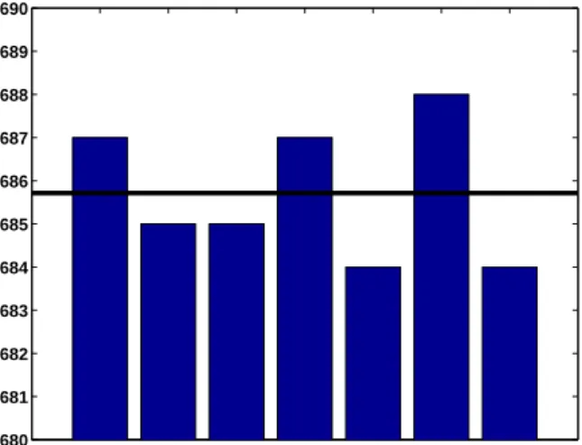
Friday the 13th is unlucky, but is it unlikely? What is the probability that the 13th day of any month falls on a Friday? The quick answer is 1/7, but that is not quite right. The following code counts the number of times that Friday occurs on the various weekdays in a 400 year calendar cycle and produces figure 3.1. (You can also runfriday13yourself.)

Su M Tu W Th F Sa 680 681 682 683 684 685 686 687 688 689 690

Figure 3.1. The 13th is more likely to be on Friday than any other day.

c = zeros(1,7); for y = 1601:2000 for m = 1:12 d = datenum([y,m,13]); w = weekday(d); c(w) = c(w) + 1; end end c bar(c) axis([0 8 680 690]) avg = 4800/7;

line([0 8], [avg avg],’linewidth’,4,’color’,’black’) set(gca,’xticklabel’,{’Su’,’M’,’Tu’,’W’,’Th’,’F’,’Sa’}) c =

687 685 685 687 684 688 684

So the 13th day of a month is more likely to be on a Friday than any other day of the week. The probability is688/4800 = .143333. This probability is close to, but slightly larger than,1/7 = .142857.

Biorhythms

Biorhythms were invented over 100 years ago and entered our popular culture in the 1960s. You can still find many Web sites today that offer to prepare personalized biorhythms, or that sell software to compute them. Biorhythms are based on the notion that three sinusoidal cycles influence our lives. The physical cycle has a

37 period of 23 days, the emotional cycle has a period of 28 days, and the intellectual cycle has a period of 33 days. For any individual, the cycles are initialized at birth. Figure 3.2 is my biorhythm, which begins on August 17, 1939, plotted for an eight-week period centered around the date this is being revised, July 27, 2011. It shows that I must be in pretty good shape. Today, I am near the peak of my intellectual cycle, and my physical and emotional cycles peaked on the same day less than a week ago.

06/29 07/06 07/13 07/20 07/27 08/03 08/10 08/17 08/24 −100 −50 0 50 100 07/27/11 birthday: 08/17/39 Physical Emotional Intellectual Figure 3.2. My biorhythm.

A search of the United States Government Patent and Trademark Office database of US patents issued between 1976 and 2010 finds 147 patents that are based upon or mention biorhythms. (There were just 113 in 2007.) The Web site is

http://patft.uspto.gov

The date and graphics functions in_Matlabmake the computation and dis-play of biorhythms particularly convenient. The following code segment is part of our programbiorhythm.mthat plots a biorhythm for an eight-week period centered on the current date.

t0 = datenum(’Aug. 17, 1939’) t1 = fix(now); t = (t1-28):1:(t1+28); y = 100*[sin(2*pi*(t-t0)/23) sin(2*pi*(t-t0)/28) sin(2*pi*(t-t0)/33)]; plot(t,y)

You see that the time variable tis measured in days and that the trig functions take arguments measured in radians.

When is Easter?

Easter Day is one of the most important events in the Christian calendar. It is also one of the most mathematically elusive. In fact, regularization of the observance of Easter was one of the primary motivations for calendar reform. The informal rule is that Easter Day is the first Sunday after the first full moon after the vernal equinox. But the ecclesiastical full moon and equinox involved in this rule are not always the same as the corresponding astronomical events, which, after all, depend upon the location of the observer on the earth. Computing the date of Easter is featured in Don Knuth’s classic The Art of Computer Programming and has consequently become a frequent exercise in programming courses. Our _Matlab version of Knuth’s program, easter.m, is the subject of several exercises in this chapter.

Recap

%% Calendar Chapter Recap

% This is an executable program that illustrates the statements % introduced in the Calendar Chapter of "Experiments in MATLAB". % You can access it with

%

% calendar_recap % edit calendar_recap % publish calendar_recap %

% Related EXM programs %

% biorhythm.m % easter.m % clockex.m % friday13.m %% Clock and fprintf

format bank c = clock f = ’%6d %6d %6d %6d %6d %9.3f\n’ fprintf(f,c); %% Modular arithmetic y = c(1)

is_leapyear = (mod(y,4) == 0 && mod(y,100) ~= 0 || mod(y,400) == 0) %% Date functions

c = clock;

dnum = datenum(c) dnow = fix(now)

39

xmas = datenum(c(1),12,25) days_till_xmas = xmas - dnow [~,wday] = weekday(now) %% Count Friday the 13th’s

c = zeros(1,7); for y = 1:400 for m = 1:12 d = datenum([y,m,13]); w = weekday(d); c(w) = c(w) + 1; end end format short c %% Biorhythms bday = datenum(’8/17/1939’) t = (fix(now)-bday) + (-28:28); y = 100*[sin(2*pi*t/23) sin(2*pi*t/28) sin(2*pi*t/33)]; plot(t,y) axis tight

Exercises

3.1Microcentury. The optimum length of a classroom lecture is one microcentury. How long is that?

3.2 π·107_{. A good estimate of the number of seconds in a year is π·10}7_{. How}

accurate is this estimate?

3.3datestr. What does the following program do? for k = 1:31

disp(datestr(now,k)) end

3.4calendar(a) What does thecalendarfunction do? (If you have the Financial Toolbox,help calendarwill also tell you about it.) Try this:

y = your birth year % An integer, 1900 <= y <= 2100. m = your birth month % An integer, 1 <= m <= 12.

calendar(y,m)

(b) What does the following code do? c = sum(1:30); s = zeros(12,1); for m = 1:12 s(m) = sum(sum(calendar(2011,m))); end bar(s/c) axis([0 13 0.80 1.15])

3.5Another clock. What does the following program do? clf set(gcf,’color’,’white’) axis off t = text(0.0,0.5,’ ’,’fontsize’,16,’fontweight’,’bold’); while 1 s = dec2bin(fix(86400*now)); set(t,’string’,s) pause(1) end Try help dec2bin if you need help.

3.6How long? You should not try to run the following program. But if you were to run it, how long would it take? (If you insist on running it, change both3’s to 5’s.) c = clock d = c(3) while d == c(3) c = clock; end

3.7First datenum. The first countries to adopt the Gregorian calendar were Spain, Portugal and much of Italy. They did so on October 15, 1582, of the new calendar. The previous day was October 4, 1582, using the old, Julian, calendar. So October 5 through October 14, 1582, did not exist in these countries. What is the_Matlab serial date number for October 15, 1582?

3.8Future datenum’s. Usedatestrto determine whendatenumwill reach 750,000. When will it reach 1,000,000?

41 3.9Your birthday. On which day of the week were you born? In a 400-year Grego-rian calendar cycle, what is the probability that your birthday occurs on a Saturday? Which weekday is the most likely for your birthday?

3.10Ops per century. Which does more operations, a human computer doing one operation per second for a century, or an electronic computer doing one operation per microsecond for a minute?

3.11Julian day. The Julian Day Number (JDN) is commonly used to date astro-nomical observations. Find the definition of Julian Day on the Web and explain why

JDN = datenum + 1721058.5

In particular, why does the conversion include an 0.5 fractional part?

3.12Unix time. The Unix operating system and POSIX operating system standard measure time in seconds since 00:00:00 Universal time on January 1, 1970. There are86,400seconds in one day. Consequently, Unix time,time_t, can be computed inMatlab with

time_t = 86400*(datenum(y,m,d) - datenum(1970,1,1))

Some Unix systems store the time in an 32-bit signed integer register. When will time_texceed 231 and overflow on such systems.

3.13Easter.

(a) The comments in easter.m use the terms “golden number”, “epact”, and “metonic cycle”. Find the definitions of these terms on the Web.

(b) Plot abargraph of the dates of Easter during the 21-st century.

(c) How many times during the 21-st century does Easter occur in March and how many in April?

(d) On how many different dates can Easter occur? What is the earliest? What is the latest?

(e) Is the date of Easter a periodic function of the year number? 3.14Biorhythms.

(a) Usebiorhythmto plot your own biorhythm, based on your birthday and centered around the current date.

(b) All three biorhythm cycles start at zero when you were born. When do they return to this initial condition? Compute them, the least common multiple of 23, 28, and 33.

m = lcm(lcm(23,28),33) Now try

What is special about this biorhythm? How old were you, or will you be, m days after you were born?

(c) Is it possible for all three biorhythm cycles to reach their maximum at exactly the same time? Why or why not? Try

t = 17003

biorhythm(fix(now)-t)

What is special about this biorhythm? How many years istdays? At first glance, it appears that all three cycles are reaching maxima at the same time,t. But if you look more closely at

sin(2*pi*t./[23 28 33])

you will see that the values are not all exactly 1.0. At what times neart = 17003 do the three cycles actually reach their maxima? The three times are how many hours apart? Are there any other values of t between 0 and the least common multiple,m, from the previous exercise where the cycles come so close to obtaining a simultaneous maximum? This code will help you answer these questions.

m = lcm(lcm(23,28),33); t = (1:m)’;

find(mod(t,23)==6 & mod(t,28)==7 & mod(t,33)==8)

(d) Is it possible for all three biorhythm cycles to reach their minimum at exactly the same time? Why or why not? When do they nearly reach a simultaneous minimum? 16−Sep−2010 16−Sep−2010 16−Sep−2010 16−Sep−2010 16−Sep−2010 16−Sep−2010 16−Sep−2010 16−Sep−2010 16−Sep−2010 16−Sep−2010 16−Sep−2010 16−Sep−2010 16−Sep−2010 16−Sep−2010 16−Sep−2010 16−Sep−2010 16−Sep−2010 16−Sep−2010 16−Sep−2010 16−Sep−2010 16−Sep−2010 16−Sep−2010 16−Sep−2010 16−Sep−2010 16−Sep−2010 16−Sep−2010 Figure 3.3. clockex

3.15clockex. This exercise is about the clockexprogram in our exmtoolbox and shown in figure 3.3.

43 (b) Makeclockexrun counter-clockwise.

(c) Why do the hour and minute hands inclockexmove nearly continuously while the second hand moves in discrete steps.

(d) The second hand sometime skips two marks. Why? How often? (e) Modifyclockexto have a digital display of your own design.

Chapter 4

Matrices

Matlab began as a matrix calculator.

The Cartesian coordinate system was developed in the 17th century by the French mathematician and philosopher Ren´e Descartes. A pair of numbers corre-sponds to a point in the plane. We will display the coordinates in avector of length two. In order to work properly with matrix multiplication, we want to think of the vector as acolumn vector, So

x=

(

x1

x2 )

denotes the pointxwhose first coordinate isx1 and second coordinate isx2. When

it is inconvenient to write a vector in this vertical form, we can anticipate_Matlab notation and use a semicolon to separate the two components,

x= (x1; x2 )

For example, the point labeledxin figure 4.1 has Cartesian coordinates x= ( 2; 4 )

Arithmetic operations on the vectors are defined in natural ways. Addition is defined by x+y= ( x1 x2 ) + ( y1 y2 ) = ( x1+y1 x2+y2 )

Multiplication by a single number, orscalar, is defined by sx=

(

sx1

sx2 )

Copyright c⃝2011 Cleve Moler

Matlab⃝R is a registered trademark of MathWorks, Inc.TM

October 4, 2011

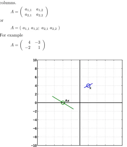
A 2-by-2 matrix is an array of four numbers arranged in two rows and two columns. A= ( a1,1 a1,2 a2,1 a2,2 ) or A= (a1,1 a1,2; a2,1 a2,2 ) For example A= ( 4 −3 −2 1 ) −10 −8 −6 −4 −2 0 2 4 6 8 10 −10 −8 −6 −4 −2 0 2 4 6 8 10 x Ax

Figure 4.1. Matrix multiplication transforms lines through x to lines through Ax.

Matrix-vector multiplication by a 2-by-2matrix Atransforms a vectorxto a vectorAx, according to the definition

Ax= ( a1,1x1+a1,2x2 a2,1x1+a2,2x2 ) For example ( 4 −3 −2 1 ) ( 2 4 ) = ( 4·2−3·4 −2·2 + 1·4 ) = ( −4 0 )

The point labeledx in figure 4.1 is transformed to the point labeled Ax. Matrix-vector multiplications producelinear transformations. This means that for scalars sandtand vectorsxandy,

47 This implies that points nearxare transformed to points nearAxand that straight lines in the plane throughxare transformed to straight lines throughAx.

Our definition of matrix-vector multiplication is the usual one involving the dot product of therows ofA, denotedai,:, with the vectorx.

Ax=

(

a1,:·x

a2,:·x )

An alternate, and sometimes more revealing, definition useslinear combinations of thecolumns ofA, denoted bya:,j.

Ax=x1a:,1+x2a:,2 For example ( 4 −3 −2 1 ) ( 2 4 ) = 2 ( 4 −2 ) + 4 ( −3 1 ) = ( −4 0 )

Thetranspose of a column vector is a row vector, denoted byxT_{. The} trans-pose of a matrix interchanges its rows and columns. For example,

xT = ( 2 4 ) AT = ( 4 −2 −3 1 )

Vector-matrix multiplication can be defined by xTA=ATx

That is pretty cryptic, so if you have never seen it before, you might have to ponder it a bit.

Matrix-matrix multiplication,AB, can be thought of as matrix-vector multi-plication involving the matrixAand the columns vectors fromB, or as vector-matrix multiplication involving the row vectors fromA and the matrixB. It is important to realize thatABis not the same matrix asBA.

Matlab started its life as “Matrix Laboratory”, so its very first capabilities involved matrices and matrix multiplication. The syntax follows the mathematical notation closely. We use square brackets instead of round parentheses, an asterisk to denote multiplication, and x’ for the transpose of x. The foregoing example becomes x = [2; 4] A = [4 -3; -2 1] A*x This produces x = 2 4

A = 4 -3 -2 1 ans = -4 0

The matricesA’*A andA*A’are not the same. A’*A = 20 -14 -14 10 while A*A’ = 25 -11 -11 5 The matrix I= ( 1 0 0 1 )

is the 2-by-2 identity matrix. It has the important property that for any 2-by-2 matrixA,

IA=AI=A

Originally,_Matlab variable names were not case sensitive, so iand Iwere the same variable. Since i is frequently used as a subscript, an iteration index, andsqrt(-1), we could not useIfor the identity matrix. Instead, we chose to use the sound-alike word eye. Today, _Matlab is case sensitive and has many users whose native language is not English, but we continue to useeye(n,n) to denote then-by-nidentity. (The Metro in Washington, DC, uses the same pun – “I street” is “eye street” on their maps.)

2-by-2 Matrix Transformations

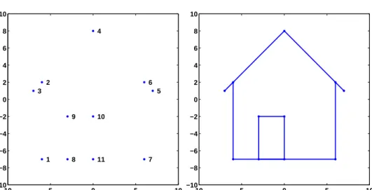
Theexmtoolbox includes a functionhouse. The statement X = house

produces a 2-by-11 matrix, X =

-6 -6 -7 0 7 6 6 -3 -3 0 0

-7 2 1 8 1 2 -7 -7 -2 -2 -7

The columns ofXare the Cartesian coordinates of the 11 points shown in figure 4.2. Do you remember the “dot to dot” game? Try it with these points. Finish off by connecting the last point back to the first. The house in figure 4.2 is constructed fromXby

49 −10 −5 0 5 10 −10 −8 −6 −4 −2 0 2 4 6 8 10 1 2 3 4 5 6 7 8 9 10 11 −10 −5 0 5 10 −10 −8 −6 −4 −2 0 2 4 6 8 10

Figure 4.2. Connect the dots.

dot2dot(X)

We want to investigate how matrix multiplication transforms this house. In fact, if you have your computer handy, try this now.

wiggle(X)

Our goal is to see howwiggleworks. Here are four matrices.

A1 = 1/2 0 0 1 A2 = 1 0 0 1/2 A3 = 0 1 1/2 0 A4 = 1/2 0 0 -1

Figure 4.3 uses matrix multiplicationA*Xanddot2dot(A*X)to show the effect of the resulting linear transformations on the house. All four matrices are diagonal or antidiagonal, so they just scale and possibly interchange the coordinates. The coordinates are not combined in any way. The floor and sides of the house remain at

−10 0 10 −10 −5 0 5 10 A1 −10 0 10 −10 −5 0 5 10 A2 −10 0 10 −10 −5 0 5 10 A3 −10 0 10 −10 −5 0 5 10 A4

Figure 4.3. The effect of multiplication by scaling matrices.

right angles to each other and parallel to the axes. The matrixA1shrinks the first coordinate to reduce the width of the house while the height remains unchanged. The matrixA2shrinks the second coordinate to reduce the height, but not the width. The matrixA3interchanges the two coordinates while shrinking one of them. The matrixA4shrinks the first coordinate and changes the sign of the second.

Thedeterminant of a 2-by-2 matrix A= ( a1,1 a1,2 a2,1 a2,2 ) is the quantity a1,1a2,2−a1,2a2,1

In general, determinants are not very useful in practical computation because they have atrocious scaling properties. But 2-by-2 determinants can be useful in under-standing simple matrix properties. If the determinant of a matrix is positive, then multiplication by that matrix preserves left- or right-handedness. The first two of our four matrices have positive determinants, so the door remains on the left side of the house. The other two matrices have negative determinants, so the door is transformed to the other side of the house.

The_Matlab functionrand(m,n)generates an m-by-nmatrix with random entries between 0 and 1. So the statement

51

R = 2*rand(2,2) - 1

generates a 2-by-2 matrix with random entries between -1 and 1. Here are four of them. R1 = 0.0323 -0.6327 -0.5495 -0.5674 R2 = 0.7277 -0.5997 0.8124 0.7188 R3 = 0.1021 0.1777 -0.3633 -0.5178 R4 = -0.8682 0.9330 0.7992 -0.4821 −10 0 10 −10 −5 0 5 10 R1 −10 0 10 −10 −5 0 5 10 R2 −10 0 10 −10 −5 0 5 10 R3 −10 0 10 −10 −5 0 5 10 R4

Figure 4.4 shows the effect of multiplication by these four matrices on the house. Matrices R1 and R4 have large off-diagonal entries and negative determinants, so they distort the house quite a bit and flip the door to the right side. The lines are still straight, but the walls are not perpendicular to the floor. Linear transformations preserve straight lines, but they do not necessarily preserve the angles between those lines. MatrixR2is close to a rotation, which we will discuss shortly. Matrix R3is nearlysingular; its determinant is equal to 0.0117. If the determinant were exactly zero, the house would be flattened to a one-dimensional straight line.

The following matrix is aplane rotation. G(θ) =

(

cosθ −sinθ sinθ cosθ

)

We use the letter Gbecause Wallace Givens pioneered the use of plane rotations in matrix computation in the 1950s. Multiplication byG(θ) rotates points in the plane through an angleθ. Figure 4.5 shows the effect of multiplication by the plane rotations withθ= 15◦, 45◦, 90◦, and 215◦.

−10 0 10 −10 −5 0 5 10 G15 −10 0 10 −10 −5 0 5 10 G45 −10 0 10 −10 −5 0 5 10 G90 −10 0 10 −10 −5 0 5 10 G215

Figure 4.5. The affect of multiplication by plane rotations though 15◦, 45◦,90◦, and215◦.

G15 =

53 0.2588 0.9659 G45 = 0.7071 -0.7071 0.7071 0.7071 G90 = 0 -1 1 0 G215 = -0.8192 0.5736 -0.5736 -0.8192

You can see that G45is fairly close to the random matrix R2seen earlier and that its effect on the house is similar.

Matlabgenerates a plane rotation for angles measured in radians with

G = [cos(theta) -sin(theta); sin(theta) cos(theta)] and for angles measured in degrees with

G = [cosd(theta) -sind(theta); sind(theta) cosd(theta)]

Our exmtoolbox function wiggle uses dot2dot and plane rotations to pro-duce an animation of matrix multiplication. Here iswiggle.m, without the Handle Graphics commands. function wiggle(X) thetamax = 0.1; delta = .025; t = 0; while true

theta = (4*abs(t-round(t))-1) * thetamax;

G = [cos(theta) -sin(theta); sin(theta) cos(theta)] Y = G*X;

dot2dot(Y); t = t + delta; end

Since this version does not have a stop button, it would run forever. The variablet advances steadily by increment ofdelta. Astincreases, the quantityt-round(t) varies between−1/2 and 1/2, so the angleθ computed by

theta = (4*abs(t-round(t))-1) * thetamax;

varies in a sawtooth fashion between-thetamaxandthetamax. The graph ofθ as a function of t is shown in figure 4.6. Each value of θ produces a corresponding plan