Pattern extraction and clustering for high-dimensional discrete data

(1)

c

(2)

PATTERN EXTRACTION AND CLUSTERING FOR HIGH-DIMENSIONAL DISCRETE DATA

BY PENG JIANG

DISSERTATION

Submitted in partial fulfillment of the requirements for the degree of Doctor of Philosophy in Computer Science

in the Graduate College of the

University of Illinois at Urbana-Champaign, 2013

Urbana, Illinois

Doctoral Committee:

Professor Michael T. Heath, Chair Professor Chengxiang Zhai

Professor Haesun Park, Georgia Institute of Technology Associate Professor Luke Olson

(3)

Abstract

We explore connections of low-rank matrix factorizations with interesting problems in data mining and machine learning. We propose a framework for solving several low-rank matrix factorization problems, including binary matrix factorization, constrained binary matrix factorization, weighted constrained binary matrix factorization, densestk-subgraph, and or-thogonal nonnegative matrix factorization. These combinatorial problems are NP-hard. Our goal is to develop effective approximation algorithms with good theoretical properties and apply them to solve various real application problems. We reformulate each of the problems as a special clustering problem that has the same optimal solution as the corresponding original problem. Making use of this property, we develop clustering algorithms to solve corresponding low-rank matrix factorization problems. We prove that most of our cluster-ing algorithms have constant approximation ratios, which is a highly desirable property for NP-hard problems. We apply the proposed algorithms and compare them with existing methods for real applications in pattern extraction, document clustering, transaction data mining, recommender systems, bicluster discovery in gene expression data, social network mining, and image representation.

(4)

Acknowledgments

I would like to give great thanks to my Ph.D. advisor Prof. Michael T. Heath for his patience, trust, understanding, and guidance. He has been very supportive of my research, giving me much freedom to attend various academic conferences. He is very knowledgable and provided insightful advice about my research. He is the best advisor I could ever have for my Ph.D. study. I am also grateful to Prof. Jiawei Han for answering my questions related to data mining and connecting me with his group. I also would like to thank my other committee members, Prof. Haesun Park, Prof. Chengxiang Zhai, and Prof. Luke Olson for their valuable feedback on my research.

I am thankful to numerous people for sharing their ideas. I thank Prof. Jiming Peng of the Department of Industrial and Enterprise Systems Engineering for discussing optimiza-tion models, Prof. Sariel Har-Peled of the Department of Computer Science for sharing his thoughts on densest k-subgraph problem, Mingjie Qian of Text Information Management and Analysis Group and Jie Chen of Argonne National Laboratory for discussing applica-tions of densest k-subgraph problem, and Jialu Liu from Prof. Han’s group for discussing advantages of Binary Matrix Factorization over Nonnegative Matrix Factorization. I ap-preciate conversations with my colleagues in the Scientific Computing Group: Mark Gates, Elena Caraba, Dmitry Yershov, Jehanzeb Hameed Chaudhry, Nana Arizumi, and Matthew Michelotti.

Last but not the least, I would like to thank my mother Ronghua Hu, my father Fanrong Jiang, my sister Dong Jiang, my husband Feng Yue, my daughter Grace Yue, and my parents-in-law Yilan Huang and Zecheng Yue for their unconditional support and love.

(5)

Chapter 1

Introduction

1.1

Motivation

With unprecedented technological advances, it is much easier and cheaper to collect and store large amounts of data. For example, rapid growth of digital imaging makes it possible to store huge numbers of radiology images for patients, leading to a large database of medical data. These huge datasets arise in many other areas such as e-commerce, computational biology, financial analysis, and image processing. In many of these applications the datasets exhibit discrete attributes. As an example, a bookstore might have millions of transactions recording customers’ book-buying behavior. Each transaction is a binary vector whose entry is one if a person buys a certain book, and zero otherwise.

These datasets contain much useful underlying information. For example, in medical research, comparions of large databases of healthy and unhealthy patients contribute to a better understanding of pathologies. Bookstores recommend books to customers by mining large databases of previous customers’ purchase history and finding relationships between books, for example, if a customer buys a book about programming, he or she is likely to buy another one about data structures. Thus it is essential to seek effective techniques to analyze these datasets.

However, these high-dimensional discrete datasets pose great challenges in data analysis due to the combination of binary features and high dimensionality. Specifically, the analysis of binary data generally leads to NP-hard problems. The high dimensionality brings several difficulties for data analysis: the computational cost is often high, clustering data items is

(8)

particularly challenging [13, 74, 92], and the curse of dimensionality is severe when model-ing high-dimensional binary data, as the number of possible combinations of the variables explodes exponentially [16]. More adaptive methods are required to address these issues.

1.2

Problem Statement

Two main tasks for analyzing high-dimensional datasets are pattern extraction and cluster-ing. Pattern extraction is essential for analyzing these datasets so as to approximate them by much smaller datasets, which reveals underlying dominant patterns in original data. It is also essential to group data into clusters. Cluster analysis has been used in many areas, such as grouping related documents for browsing, or finding genes and proteins that have similar functionalities. To perform these two tasks, we use low-rank matrix factorization to approximate the original matrix by a product of two low-rank matrices.

A fundamental result of linear algebra states that for any given matrix G and positive integer k, and any rotation-invariant norm (e.g., Frobenius norm and 2-norm), there is a matrix Gk that minimizes kG−Gkk over all matrices Gk of rank k. Low-rank matrix ap-proximations have long been studied by numerical analysts but have only recently received broader attention in computer science due to their usefulness in areas such as machine learning, computer vision, and information retrieval, for which they are used for extracting correlations and removing noise from matrix-structured data, compression of single images and multiple spectral image cubes, and latent semantic indexing for large document collec-tions. For a more complete list of applications of matrix decompositions in data mining, see Skillicorn [88].

(9)

Mathematically, given a matrix G ∈ _Rm×n _{and a positive integer} _k _{min(m, n),} con-strained low-rank matrix approximation can be formulated as

min U,W kG−U Wk 2 F (1.1) s.t. U ∈_Rm×k_, _W _∈ Rk×n, U ∈Cu, W ∈Cw,

whereCuandCw are the feasible sets forU andW, respectively. Many well-known problems have the form (1.1), including singular value decomposition (SVD) and nonnegative matrix factorization (NMF). Our target is four other interesting problems: binary matrix factoriza-tion (BMF), constrained binary matrix factorization (CBMF), weighted constrained binary matrix factorization (WCBMF), anddensestk-subgraph (DkS), among which BMF and DkS are popular existing problems, whereas CBMF and WCBMF are new problems proposed by us. BMF aims to approximate a binary matrix by a product of two low-rank binary matrices. Binary datasets occupy a special place in data analysis [67]. In the previous literature on BMF, the matrix product is not required to be binary. We call this unconstrained BMF (UBMF). Since the matrix Gis binary, it is often desirable to have a matrix product that is also binary. We call the resulting constrained problem CBMF. In this thesis, BMF refers to either UBMF or CBMF. We further propose our weighted CBMF (WCBMF) model inspired by the fact that there are two different types of mismatched entries between the original ma-trix and the product mama-trix: 0-becoming-1 and 1-becoming-0, and CBMF aims to minimize the sum of the two types of mismatched entries with no preference for minimizing a specific type. WCBMF is a generalization of CBMF that takes a different penalty weight for each type of error. DkS aims to find a k-vertex induced subgraph having the maximum number of edges (or edge weight) for a given (weighted) graph. It is not immediately obvious that DkS fits the pattern of (1.1), but we reformulate DkS as a single clustering problem, which can then be formulated as a constrained rank-one matrix factorization.

(10)

Alternating iterative algorithms are widely used to solve continuous optimization prob-lems of the form (1.1). This is because the objective function kG−U Wk2

F is convex in either W or H separately, but not convex in both variables simultaneously. Thus one ex-pects to find local minima instead of global minima. The algorithm requires solving two subproblems: To minimize or reduce the ojective function, first find W for fixed U and then U for this value of W, and repeat. Let f(U,W) = kG−U Wk2

F. We present an alternating iterative algorithm template for problems of form (1.1).

Algorithm 1: Alternating Iterative Algorithm Template for form (1.1) 1 Repeat the following steps I times:

input :G∈ {0,1}m×n_{, and initial random matrix} _U _{∈ {0,}_1}m×k output:U ∈ {0,1}m×k _and _W _{∈ {0,}_1}k×n _{that reduce}_f₍_U_,_W₎ 2 repeat

3 For this fixed U, find W to minimize or reduce f; 4 For this fixed W, find U to minimize or reduce f; 5 until objective value does not decrease;

6 Return U and W with minimum objective value over allI runs.

Algorithm 1 provides a template for computing various approximate factorizations having the form (1.1), which may differ in the methods and costs for solving the two subproblems. This thesis focuses on a class of combinatorial factorizations whose subproblems can be reformulated as specific clustering problems, for which there are many existing effective approximation algorithms.

1.3

Prior Work

Numerous techniques have been proposed to deal with continuous data. Singular value de-composition (SVD) decomposesGintoG=UΣVT_{, where}_U _and_V _{are orthogonal matrices,} and Σ is a diagonal matrix with singular values in descending order. A rank-one approx-imation to G can be obtained by the outer product of the first column in U and the first column in V scaled by the first singular value in Σ. Similarly, a rank-k approximation can

(11)

be obtained by the sum ofk decreasingly significant rank-one matrices. This truncated SVD is the optimal solution for minimizing the error defined in Frobenius norm. This result is originally due to Eckart and Young [35]; for a modern treatment in terms of the SVD, see Golub and Van Loan [43]. Conventional algorithms for computing the full SVD are pro-hibitively expensive for large matrices, but a useful partial SVD can be computed relatively cheaply using orthogonal iteration or Lanczos iteration [43], which require only repeated matrix-vector multiplications. Methods for reducing the cost include sampling [32, 38] and Lanczos bidiagonalization [87].

Principal Direction Divisive Partitioning (PDPP)[18] is a hierarchical clustering strategy for high-dimensional sparse datasets. It partitions the original dataset into two parts based on the direction of the first singular vector obtained by SVD, and then recursively partitions the resulting datasets. This results in a binary tree that partitions data in ways that reflect the most important variation.

CUR Decomposition [73] approximates the original matrix G by a product of three matrices CU R, where C is a set of columns of G, and R is a set of rows of G. Usually CUR Decomposition is selected to be a rank-k approximation, whereC contains k columns of G, R contains k rows of G, and U is a k×k matrix. CUR Decomposition provides a high-quality sketch of the original data, but is much smaller and thus easier to analyze in practice.

NMF factorizes a nonnegative matrix into a product of two nonnegative matrices. The most popular approach to solving NMF is the multiplicative update algorithm proposed by Lee and Seung [66]. Other successful algorithms include the projected gradient descent method [69], active-set method [57], and block principal pivoting method [58].

Semidiscrete Decomposition (SDD) [60] is a more space efficient version of SVD. The entries of U and V can be only 0, 1, or −1, thus saving much storage space compared with SVD. The performance of SDD in the application of latent semantic indexing is comparable to truncated SVD, while reducing the storage to one-tenth [59].

(12)

However, approximation data obtained by all these methods still contain negative and non-binary values, from which it is hard to deduce useful information to help understand the original binary data. We need algorithms specially designed for discrete data, for which there have been relatively few alternating iterative algorithms. Zhang et al. [99, 100] pro-posed a penalty function and thresholding algorithm to update U and W iteratively for rank-k BMF. Most such works, e.g., [61, 70, 86], are mainly concerned with rank-one ap-proximation, in which case a rank-k BMF is then computed by partitioning the data set at each stage and repeating the rank-one factorization for each submatrix. Algorithms have been proposed for DkS based on a variety of techniques, including greedy algorithms [15, 24], linear programming [17, 55], and semidefinite programming [91, 97]. However, there have been no alternating iterative algorithms for DkS because it has not previously been cast in the form (1.1).

In addition, the discrete features in the datasets generally lead to NP-hard problems and there are few discussions about approximation ratios of existing algorithms for these problems. For example, Shen et al. [86] proved that their rank-one algorithm has an ap-proximation ratio of 2, but there is no apap-proximation ratio known for rank-k BMF. No constant-factor approximation algorithm for DkS has been reported in the literature.

1.4

Objective

In this thesis, we mainly consider discrete optimization problems. Our goals are to (i) provide a framework in which many well-known problems can be formulated, as well as new problems we introduce, such as CBMF and WCBMF. This framework allows us to apply alternating iterative algorithms, which require solving two subproblems; (ii) propose effective clustering methods to solve the subproblems. We find that the discrete properties allow us to reformulate each subproblem as a specific clustering problem, for which there are many existing effective approximation algorithms; (iii) prove that most of our proposed algorithms

(13)

have approximation ratio of 2 for the reformulated clustering problems, which have the same optimal solutions as the original discrete optimization problems. The 2-approximation is theoretically significant, as the original problems are usually NP-hard with few, if any, constant factor approximation algorithms reported; (iv) apply our algorithms to numerous applications in data mining and machine learning, mainly concerning pattern extraction and clustering for high-dimensional datasets; and (v) identify additional problems that can fit into this framework and whose corresponding subproblems can be solved by algorithms with good theoretical properties.

We describe BMF, WCBMF, and DkS in Chapter 2, 3, and 4 respectively. For each problem, we reformulate it as a specific clustering problem, propose clustering algorithms, discuss their approximation ratios, and apply them to interesting applications.

Besides these discrete optimization problems, we observe that a variant of a continuous optimization problem, NMF, can also be cast in our framework. The problem is called

orthogonal nonnegative matrix factorization (ONMF), which adds one more constraint to NMF, enforcing orthogonality constraints on columns ofU or rows ofW. The orthogonality constraint enables us to reformulate ONMF as a variant of a weighted clustering problem, as described in Chapter 5.

(14)

Chapter 2

Binary Matrix Factorization

2.1

Introduction

High-dimensional binary datasets arise in many areas such as business, bioinformatics, and image processing. For example, a supermarket might have millions of transactions recording customers’ grocery-buying behavior. Note that binary datasets means that only values 0 and 1 are allowed. As introduced in Chapter 1, these datasets pose great challenges in data analysis due to the combination of high dimensionality and binary features. Chapter 1 describes many methods for analyzing continuous data, but the approximation data obtained by all these methods still contains negative and non-binary values, from which it is difficult to deduce useful information to help understand the original binary data. Moreover, each of these real-valued entries is typically stored in 32 or 64 bits, while each binary entry needs only 1 bit to store.

In order to address these issues, we propose clustering algorithms for binary matrix factorization (BMF) to compress the data and extract dominant patterns. In the existing literature, BMF is defined as follows: given a binary matrix G∈ {0,1}m×n_{, BMF finds two} binary matricesU ∈ {0,1}m×k _and _W _{∈ {0,}_1}k×n _{so that the distance between} _G_{and the} matrix product U W is minimal. Conventionally, the distance is measured by the square of the Frobenius norm, leading to an objective functionkG−U Wk2

F. BMF has applications in many areas, such as document clustering [99], association rule mining [62], pattern discovery for gene expression pattern images [86], digits reconstruction for USPS datasets [76], market basket data clustering [67].

(15)

In 2002, Koyut¨urk et al. [61] proposed PROXIMUS to approximate a binary dataset by another one with low rank. It finds a rank-one approximation to the original binary data and then performs recursive partitioning until some stopping criterion is met and the algorithm stops at a certain rank. PROXIMUS was the first algorithm for BMF. Koyut¨urk et al. [62] further showed that BMF is NP-hard because it can be formulated as an integer programming problem with 2m+nfeasible solutions, even for rank-1 BMF. They showed that there is no theoretical guarantee on the quality of the solution produced by PROXIMUS [63]. Lin et al. [70] proposed an algorithm theoretically equivalent to PROXIMUS but with lower computation cost. Shen et al. [86] proposed a 2-approximation algorithm for rank-1 BMF by reformulating it as a 0-1 integer linear problem (ILP). Gillis and Glineur [40] gave an upper bound for BMF by finding the maximum edge bicliques in the bipartite graph whose adjacency matrix isG. They also proved that rank-1 BMF is NP-hard. Miettinen et al. [77] defined discrete basis problem (DBP) as another way to approximate a binary matrix by the boolean product of two binary matricesU ⊗W so as to minimize kG−U ⊗Wk(1,1). They

also considered a special variant of DBP, which adds another constraint that each column of

W has exactly one entry of value 1. They named this problem Discrete Basis Partitioning Problem (DBPP) and showed that there exists a 10-approximation algorithm for it. As we will see later, DBPP can be viewed as a more restrictive version of BMF.

Note that though the definition of BMF does not require matrix product U W to be binary, all existing methods for BMF produce a binary matrix product, as it is desirable to approximate a binary matrix by another binary one in many real applications. This extra constraint on matrix product would produce more sparse matrix factors U and W, and greatly reduce the computational cost, as we will see later. For comparison, we call the problem unconstrained BMF (UBMF) if we do not impose the extra constraint on the matrix product, and the other problemconstrained BMF (CBMF), where the matrix product is restricted to the class of binary matrices. In this thesis, BMF refers to UBMF or CBMF.

(16)

We introduce two variants of CBMF that involve only linear constraints to ensure that the resulting matrix product is binary. We note that when the matrix product U W is binary, then there is no difference between the squared Frobenius norm and the (1,1) norm of the matrix G−U W. As shown in a recent study [20], the use of the (1,1) norm is very helpful in the pursuit of sparse solutions to various problems. Thus we use the (1,1) norm as the objective function in our BMF model. As we will see later, this will substantially affect the solution process. We explore the relationship between BMF and special classes of clustering problems and use this relation to develop an effective approximation algorithm, which we prove has approximation ratio of 2. The clustering algorithm works well for small values of k, but its complexity is exponential in k because it chooses all possible k points out of n points as initial cluster centers, and thus it is not suitable for large values of k. Therefore we propose to choosekcluster centers randomly based on preassigned probabilities to each point so that the randomized clustering algorithm works well for large values of k. We further estimate the quality of the solution. Our method differs from others such as PROXIMUS and ILP [86] in that it effectively discovers the desired number of underlying dominant patterns instead of first finding a rank-one approximation and then performing partitioning recursively. Since the approximation data represents the original dataset quite well but with much smaller size, it provides a good starting point for other purposes. For example, applying association rule mining algorithms to approximate data instead of the original data will result in high speedup in time. Our experiments show that rules mined from approximate data match the ones mined from original data quite well. In addition, we compare our method with other popular ones for document clustering and results show that our method often beats others with highest accuracy.

In addition, we propose alternating update procedures for UBMF. In every iteration of the procedure, we solve a BQP subproblem to update the matrix argument. We also explore the relationship between solutions of UBMF and CBMF and establish a sandwich theorem between them.

(17)

2.2

Problem Definition

Given G∈ {0,1}m×n _{and an integer} _k _{min(m, n), UBMF of rank} _k _{is defined as}

min

U,W ||G−U W||

2

F (2.1)

s.t. U ∈ {0,1}m×k_, _W _{∈ {0,}_1}k×n_.

Note that in the above model, the matrix product U W is not required to be binary. As pointed out in the introduction, since the matrixGis binary, it is desirable to have a binary matrix product. This leads to the problem

min U,W ||G−U W|| 2 F (2.2) s.t. U ∈ {0,1}m×k_, _W _{∈ {0,}_1}k×n_, [U W]ij ≤1, ∀ i= 1,· · · , m, j = 1,· · · , n. (2.3)

The quadratic constraint (2.3) makes the problem very hard to solve. To see this, let us temporarily fix one matrix, sayU, then we end up with a BQP with linear constraints, which is still NP-hard [23]. One way to reduce the difficulty in problem (2.2) is to replace the hard quadratic constraints by some linear constraints that will ensure the resulting matrix product remains binary. For this purpose, we introduce the following two specific variants of CBMF,

min

U,W kG−U Wk(1,1) (2.4)

s.t. U ∈ {0,1}m×k_, _W _{∈ {0,}_1}k×n_,

(18)

and

min

U,W kG−U Wk(1,1) (2.5)

s.t. U ∈ {0,1}m×k_, _W _{∈ {0,}_1}k×n_,

U ek≤em.

We replace the squared Frobenius norm by the (1,1) norm, which is defined as kGk(1,1) =

m P i=1 n P j=1

|gij|for any matrixG. Note that the two measures are the same whenU W is binary. However, we will see later that using the (1,1) norm will substantially affect the solution process. In addition, ek, em, and en are vectors of all ones in Rk, Rm, and Rn, respectively. The constraint WTek ≤en (or U ek ≤ em) ensures that every column ofW (or every row of U) contains at most one nonzero element, and thus it guarantees that U W is a binary matrix.

Next we show that the general CBMF model (2.2) is equivalent to our CBMF models when k = 2.

Proposition 2.2.1. If k = 2, then problem (2.2) is equivalent to either problem (2.4) or (2.5).

Proof. It suffices to prove that if (U,W) is a feasible pair to problem (2.2), then it must satisfy either U ek ≤ em or WTek ≤ en. Suppose to the contrary that both constraints

U ek ≤ em and WTek ≤ en do not hold, i.e., the i-th row of U and the j-th column of W satisfy

Ui1+Ui2 = 2, W1j +W2j = 2. It follows immediately that

(19)

contradicting to the assumption that (U,W) is a feasible pair for problem (2.2). Therefore, we have either U ek ≤em orWTek≤en. This completes the proof of the proposition.

We remark that Proposition 2.2.1 does not hold if k ≥ 3. This can be seen from the following example. Consider a matrix pair (U,W) defined by

U =    1 0 1 0 0 1   , W =       0 1 1 1 1 0       .

One can easily see that (U,W) is a feasible solution to problem (2.2), but it is not a feasible solution to problem (2.4) or (2.5).

2.3

BMF and Clustering

In this section, We show that CBMF is equivalent to a special class of (k+1)-means clustering problem. In addition, we explore the relationship between CBMF and several well-known clustering problems. We also reformulate UBMF as a special 2k_{-means clustering.}

2.3.1

CBMF and Clustering

We first define a special (k+ 1)-means clustering as follows:

(k+ 1)-means clustering: Given a setV of n binary points in _Rm _{and a positive integer} k with k ≤ n, find a set S = {s1,· · · , sk} of binary centers in Rm and a partition C = {C0, C1,· · · , Ck} such thatS and C minimize

k X i=1 X v∈Ci kv −sik1+ X v∈C0 kv−s0k1,

(20)

wheres0is the origin of theRm andl1norm of any vectorv ∈Rnis defined askvk1 =

n P i=1

|vi|. We name this problem (k+1)-means clustering as we partition data points intok+1 clusters. Note that cluster centersi can be any binary vector, i.e., S does not have to be a subset of V.

We show the equivalence of CBMF and the (k+ 1)-means clustering.

Theorem 2.3.1. CBMF and the (k+ 1)-means clustering are equivalent in the sense that they have the same optimal solution set and objective value.

Proof. We first show that the theorem holds for CBMF (2.4), as the proof for CBMF (2.5) follows a similar way. Note that the objective value of CBMF (2.4) can be expressed as a summation over columns, that is, kG−U Wk(1,1) = Pn_i₌₁kgi−U wik1, where gi and wi denote the i-th column of G and W, respectively. Let us temporarily fix U and consider the resulting subproblem of CBMF (2.4):

min W n X i=1 kg_i−U wik1 (2.6) s.t. eT_kwi ≤1, i= 1,· · · , n; wi ∈ {0,1}k, i= 1,· · · , n.

The solutionW to problem (2.6) can be obtained column by column, and the way to update the i-th column wi for 1≤i≤n is shown as follows:

wi(j) =        1 if uj = arg minl=1,···,kkgi−ulk1 0 otherwise ,

where wi(j) is the j-th component of wi. Note that wi updated in this way is guaranteed to be the optimal solution of (2.6) as the matrix-vector product U wi in the objective value of (2.6) is either a column of U or the origin of _Rm _{because of the constraints on} _w

i. If wi(j) = 1, we say gi is assigned to uj, otherwise gi is assigned to u0, the origin of

(21)

the space _Rm_{. Thus problem (2.6) assigns each point} _g

i to the nearest center in the set {u0,u1, . . . ,uk}. It follows that CBMF (2.4) can be cast as the following clustering problem:

min u1,...,uk n P i=1 minl=0,1,···,kkgi−ulk1 (2.7) s.t. uj ∈ {0,1}m, j = 1, . . . , k.

Note that problem (2.7) is just another formulation of the (k+ 1)-means clustering, with V = {g₁, . . . ,g_n}, S = {u1, . . . ,uk}, and C is given by solving the inner minimization

problem of (2.7).

Thus CBMF (2.4) is equivalent to the (k + 1)-means clustering with the same optimal value and optimal solution set. Specifically,U gives the centers, and W gives the partition. Similarly CBMF (2.5) can be reformulated as a (k+ 1)-means clustering problem with W

giving the centers, and U giving the partition.

We now explore the relationship between CBMF and two well-known clustering problems: k-means clustering [75] and k-medoids clustering [52]. Theorem (5.3.1) allows us to use the formulation of the (k+ 1)-means clustering instead of the CBMF model for comparison with other clustering problems. We first compare CBMF with classical k-means clustering, the definition of which is given as follows:

Classical k-means clustering: Given a set V of n binary points in _Rm and a positive integer k with k≤n, find a partitionC ={C1,· · · , Ck} such that C minimizes

k X i=1 X v∈Ci kv− P v∈Ci v |Ci| k2_.

We conclude that CBMF is very close to classicalk-means clustering with two differences: One is that in CBMF an additional center, the origin, is used in the assignment process, which allows CBMF to assign many sparse points to the origin and perform the clustering task only for the relatively dense points. Intuitively, this will help to reduce the objective

(22)

value. It is interesting to note that DBPP discussed in [77], is a restricted problem of CBMF (2.4) with constraint WT_e

k = en instead of WTek ≤ en. In other words, every column ofG must be assigned to a cluster.

Another difference between CBMF and the classical k-means clustering is that CBMF uses binary points as centers, while in classical k-means clustering, each cluster center is the geometric center of all the data points in that cluster. However, we later prove an interesting conclusion that optimal centers for CBMF are obtained by rounding geometric centers to binary ones. In addition, we use l1 norm in CBMF’s equivalent (k+ 1)-means clustering

problem, whereas squared l2 norm is used in k-means. However, the two measures are the

same for binary data.

In addition, there is a close relationship between CBMF and k-medoids clustering, the definition of which is given as follows:

k-medoids clustering: Given a set V of points in _Rm and a positive integer k with |V| = n and k ≤ n, find a set of centers S = {s1,· · ·, sk} with S ⊆ V and a partition C ={C1,· · · , Ck} such thatS and C minimize

k X i=1 X v∈Ci kv−sik1.

The definitions of the (k+ 1)-means clustering andk-medoids clustering show that CBMF is very close tok-medoids clustering with two differences: One is that CBMF has an additional center, the origin, which brings extra benefits explained earlier. Another difference is that CBMF uses any points as centers, whilek-medoids clustering chooses points from the original data points as centers, which makes it a much more restricted problem of CBMF.

2.3.2

UBMF and Clustering

We define the 2k_{-means clustering as follows:}

2k_{-means clustering:} _{Given a set}_V _of_n_{binary points in}

(23)

k ≤ n, find a set S = {s1,· · ·, sk} of k binary points in Rm to form another set S0 of all

possible linear combinations of thek points inS, i.e.,S0 ={s0

1,· · · , s 0 2k}withs 0 l = k P j=1 αl(j)sj and αl(j) ∈ {0,1}. Take the 2k points in S0 as cluster centers and find the corresponding partition C ={C1,· · · , C2k} to minimize 2k X i=1 X v∈Ci kv−s0_ik1.

We name this problem 2k_{-means clustering as we partition data points into 2}k _{clusters. We} show the equivalence of UBMF and the 2k_{-means clustering.}

Theorem 2.3.2. UBMF and the 2k-means clustering are equivalent in the sense that they have the same optimal solution set and objective value.

Proof. The objective value of UBMF (2.1) can be expressed as a summation over columns, that is, kG−U Wk2

F = Pn

i=1kgi −Uwik2. Let us temporarily fix U and consider the resulting subproblem of UBMF (2.1):

min W n X i=1 kg_i−U wik2 (2.8) s.t. wi ∈ {0,1}k, i= 1,· · · , n.

Note that the matrix-vector productU wi in the objective value is a linear combination ofk pointsu1, . . . ,uk, where the scalars are either 0 or 1. Following a similar procedure as in the proof of Theorem 5.3.1, we conclude that UBMF (2.1) is another formulation of 2k_-means clustering with V = {g₁, . . . ,g_n} and S = {u1, . . . ,uk}. We then construct S0 based on k points in S, that is, S0 = {u0₁,· · · ,u0₂k} with u

0 l = k P j=1 αl(j)uj and αl(j) ∈ {0,1}. Though

W is not explicitly defined in 2k-means clustering, it can be updated given the partition in the clustering problem. Specifically, the i-th column wi of problem (2.8) for 1≤i ≤n can

(24)

be updated as follows: wi(j) =        1 if u0_l= arg mins∈S0kg i−u 0_k _and _α l(j) = 1 0 otherwise .

2.4

Algorithms for CBMF

In this section, we present two approximation algorithms for CBMF. We first describe a deterministic 2-approximation algorithm for CBMF. The algorithm is effective for small k, but it takes too much time for large k. Thus we present a randomized clustering algorithm that chooses k cluster centers based on preassigned probabilities of each point so that it works well for large values ofk.

The key issue for a clustering algorithm is how to update the centers. We discuss how to find the optimal binary center to minimize the sum of the l1 distances within a cluster in

(k+ 1)-means clustering. Given a clusterC1 of p binary data points C1 ={v1,· · · , vp}, we find a binary center s1 to minimize the following optimization problem:

min s1

P v∈C1

kv−s1k1. (2.9)

We calls1 the l1 center of the cluster, and give the following theorem for the optimal s1.

Theorem 2.4.1. Given a cluster C1 of p binary data points, the optimal binary center of

problem (2.9) is obtained by rounding the geometric center of cluster C1 to binary.

Proof. The theorem holds because of a well-known fact that median minimizes the absolute error, which in binary vectors means that element-wise majority minimizes l1 norm.

We also give another way to show the proof. Since each component of the optimal s1

(25)

how to determine that of optimals1, denoted ass1(1). Suppose that

v1(1) =· · ·=vl(1) = 0, vl+1(1) =· · ·=vp(1) = 1,1≤l < p.

Note that points with the same values of first components are indexed together just for illustration purpose. In other words, we can always re-index the points to let the first l points have value 0 as the first components, and the other (p−l) points have value 1 as the first components. By looking at the objective value of (2.9), it is easy to see that the optimals1(1) to minimize the l1 distance should be

s1(1) =      0 if l≥p/2 1 otherwise .

On the other hand, the first component of the geometric center is simply the mean of all components vc(1) = p−l p = 1− l p.

Thuss1(1) is the rounded value ofvc(1). Similarly other entries ofs1are rounded values of the

corresponding entries of the geometric center. This completes the proof of the theorem.

2.4.1

Deterministic 2-Approximation Algorithm

There have been many effective algorithms proposed for k-means clustering. Lloyd [71] proposed an iterative refinement method that is widely used. We modify Lloyd’s algorithm for the CBMF problem. We first cast every column of G as a data point in_Rm _{and denote} the resulting data set by V, whose cardinality is n. Then we formulate another set SV(k) that contains all subsets ofV with a fixed sizek. The cardinality ofSV(k) is n_k. We obtain a clustering algorithm for CBMF (2.4) in Algorithm 2, which tries every subset inSV(k) as an initial U and returns the solution with minimum objective value over all runs.

(26)

Algorithm 2: Clustering for CBMF (2.4) 1 for l←1 to n_k do

2 Choose subset s_l ∈ S_V(k) and form initial U by casting every point ins_l as a column of U;

3 for i←1 to n do

4 Assign g_i to nearest center among u₀,u₁, . . . ,u_k; 5 for j ←1 to k do 6 if g_i is assigned to uj then 7 w_i(j) = 1; 8 else 9 wi(j) = 0; 10 end 11 end 12 end

13 Compute new l₁ center for each cluster C_p based on newly assigned data points; if there is no change in l1 center for every p= 1, . . . , k then

14 Output U and corresponding W as solution; 15 else

16 Update l₁ center for each cluster and go to line 3; 17 end

18 end

(27)

We next consider the approximation ratio of Algorithm 2.

Theorem 2.4.2. Suppose that U∗ = [u∗₁, . . . ,u∗_k] is the global optimal solution of prob-lem (2.7), with an objective value fopt, and U = [u1, . . . ,uk] is the solution output by

Algorithm 2 with an objective value f(U). Then

f(U)≤2fopt.

Proof. Let Cp denote the p-th cluster with the binary center u∗p at the optimal solution for 1 ≤ p ≤ k, and C0 the optimal cluster with center u0. Then we can rewrite the optimal

objective value of problem (2.7) as

fopt = k X p=1 X gi∈Cp kg_i−u∗_pk1 + X gi∈C0 kg_ik1. (2.10)

Letg∗_p denotes the point in Cp that is closest to the center, i.e.,

g∗_p = arg min gi∈Cp kg_i −u∗_pk1. (2.11) It follows that X g_i∈Cp kg_i−g∗_pk1 = X g_i∈Cp k(g_i−u∗_p) + (u∗_p−g∗_p)k1 ≤ X gi∈Cp (kg_i−u∗_pk1+kg∗p−u ∗ pk1) ≤ 2 X gi∈Cp kg_i−u∗_pk1, (2.12)

where the first inequality follows from the triangle inequality of l1 norm and the positive

(28)

inequality follows from (2.11). Therefore, we have f(U) ≤ k X p=1 X gi∈Cp kg_i −g∗_pk1+ X gi∈C0 kg_ik1 ≤ 2 k X p=1 X g_i∈Cp kg_i−u∗_pk1+ X g_i∈C0 kg_ik1 ≤ 2( k X p=1 X gi∈Cp kg_i−u∗_pk1+ X gi∈C0 kg_ik1) = 2fopt,

where the first inequality holds because every g∗_p for p = 1, . . . , k comes from original data points and thus these k points must be used as initial centers in Algorithm 2. The second inequality holds due to (2.12). It is straightforward to verify the third inequality, and the last equality follows from (2.10).

We conclude from Theorem 2.4.2 that CBMF (2.4) can be solved by Algorithm 2 with approximation ratio of 2, as CBMF (2.4) and problem (2.7) are equivalent problems. The time complexity is O(mnk+1_{). Similary, we can approximate CBMF (2.5) within a factor}

of 2 in time O(nmk+1_{). The approximation ratio of 2 is a desirable quality of Algorithm 2,}

especially considering that CBMF is NP-hard. However, the time complexity implies that it works effectively only for small k. In the next subsection, we discuss how to use a random starting strategy.

2.4.2

Randomized Approximation Algorithm

We present an O(logk) approximation algorithm for CBMF based on randomized centers. Instead of the exhaustive search procedure in Algorithm 2, we modify the random seed selection process in kmeans++ [14] to obtain the starting centers. LetD(v, P) denote the l1

distance from a data pointv to the closest point in a data setP. We propose a randomized clustering Algorithm.

(29)

Algorithm 3: Randomized clustering for CBMF (2.4) 1 Initialize P to contain the origin point;

2 for i←1 to k do

3 Randomly choose cluster center u_i fromV ={v₁, . . . ,v_n}where P(ui =vj) = D(vj, P)/ P

v∈V

D(v, P); 4 Add ui to P.

5 end

6 Perform steps 3-17 of Algorithm 2.

We use a weighted probability distribution where a point is chosen to be next center with probability proportional to its l1 distance from its closest existing center. For convenience,

we call the weighting used in the above procedure D1 weighting. The way we assign D1

weighting is quite reasonable, as the center that has been chosen will be assigned weight zero and thus will not be chosen again, and the next center is more likely to be chosen far away from existing centers. Once k starting centers are chosen, we continue the clustering procedure in Algorithm 2.

Next we show in the following theorem that Algorithm 3 has approximation ratio of O(logk).

Theorem 2.4.3. Suppose that fopt is the optimal objective value of problem (2.7), and U

is the solution output by randomly choosing initial centers in Algorithm 3 with an objective value f(U). Then

E(f(U))≤4(lnk+ 2)fopt.

The theorem is similar with the conclusion in [14], but we have a sharper bound on the objective value. As in [14], we need several technical results to prove it. For notational convenience, let us denoteCopt ={C0,C1,· · · ,Ck}, where everyCiis the cluster in the optimal solution associated with cluster centeru∗_i. Specifically,C0is the cluster associated with center

u0.

We first prove the following lemma for a cluster whose center is selected uniformly at random from the set itself.

(30)

Lemma 2.4.4. Let A be an arbitrary cluster in the final optimal clusters Copt, and let C be

a clustering with center selected uniformly at random from A. Then

E(f(A))≤2fopt(A).

Proof. The proof follows a similar vein as the proof of Lemma 3.2 in [14] with the exception that the Euclidean distance has been replaced by the l1 distance. Let c(A) be the l1 center

of the cluster in the optimal solution. It follows that

E(f(A)) = X a0∈A 1 |A| X a∈A ka−a0k1 ≤ 1 |A| X a0∈A X a∈A ka−c(A)k1 (2.13) + 1 |A| X a0∈A |A| · ka0−c(A)k1 = 2X a∈A ka−c(A)k1.

The inequality follows from the triangle inequality of l1 norm. It should be mentioned

that the above lemma holds for the cluster C0. In such a case, we need only to change the

l1 center c(A) to u0 in the proof of the lemma.

We then extend the above result to the remaining centers chosen with D1 weighting.

Lemma 2.4.5. Let A be an arbitrary cluster in the final optimal clusters Copt, and let C be

an arbitrary clustering. If we add a random center to C from A, chosen with D1 weighting,

then

E(f(A))≤4fopt(A).

Proof. Note that for any a0 ∈ A, the probability that a0 is selected as the center is

D(a0)/(

P

(31)

in the objective value to min(D(a),ka−a0k1). It follows that E(f(A)) = X a0∈A D(a0) P a∈AD(a) X a∈A min(D(a),ka−a0k1).

Note by the triangle inequality of l1 distance, we have that D(a0) ≤ D(a) +ka−a0k1 for

any a. Thus by summing over a, we have D(a0)≤

P a∈A(D(a)+ka−a0k1) |A| , and hence E(f(A)) ≤ 1 |A| X a0∈A P a∈A(D(a) +ka−a0k1) P a∈AD(a) X a∈A min(D(a),ka−a0k1) ≤ 1 |A| X a0∈A P a∈AD(a) P a∈AD(a) X a∈A ka−a0k1+ 1 |A| X a0∈A P a∈Aka−a0k1 P a∈AD(a) X a∈A D(a) = 2 |A| X a0∈A X a∈A ka0−ak1 ≤ 4fopt(A),

where the second inequality holds because the two relationships hold: min(D(a),ka−a0k1)≤

ka−a0k1and min(D(a),ka−a0k1)≤D(a). The last inequality follows from Lemma 2.4.4.

Lemma 2.4.5 is similar to Lemma 3.3 in [14], but we gain a closer bound on f(A) by 4, instead of 8 in [14]. This is due to the use of the (1,1) norm. It leads to a sharper bound on the objective value in Theorem 2.4.3. The following lemma resembles Lemma 3.4 in [14], with a minor difference in the constant used in the estimate. Thus we omit its proof. Lemma 2.4.6. Let C be an arbitrary clustering. Choose T > 0 ‘uncovered’ clusters from

Copt, and let Vu denote the set of points in these clusters, withVc=V − Vu. Suppose we add t≤T random centers to C, chosen with D1 weighting. Let C0 denote the resulting clustering.

Then

E(f(C0))≤(1 +Ht)(f(Vc) + 4fopt(Vu)) + T −t

T f(Vu),

(32)

Now we are ready to prove the main result in this subsection.

Proof of Theorem 2.4.3. Consider the clustering C after all the starting centers have been selected. Let A denote the cluster in Copt from which we choose u1. Applying Lemma 2.4.6

with t=T =k−1, and with C0 and A the only two possibly covered clusters, we have

E(f(C)) ≤ (f(C0) +f(A) + 4f(Copt)

−4fopt(C0)−4fopt(A))(1 +Hk−1)

≤ 4(2 + lnk)f(Copt),

where the last inequality follows from Lemma 2.4.5 and the fact thatHk−1 ≤1 + lnk.

2.5

Algorithms for UBMF

We apply the popular alternating update procedure for solving UBMF. That is, for fixedU, we findW to minimize or reduce f, and then for this value ofW, we find a value for U that minimizes or reduces f further. We repeat the procedure until the objective value does not decrease. In each iteration of the procedure, we solve a subproblem to update the matrix argument.

We propose two methods to solve the subproblems: clustering algorithm and greedy heuristic. Note that the two methods are proposed to solve the subproblem of updating W while fixing U, and the other subproblem can be solved by a similar way.

2.5.1

Clustering Algorithm for UBMF

Theorem 2.3.2 establishes the relationship between UBMF and 2k_{-means clustering, thus it} indicates a clustering assignment procedure, which is described in Algorithm 4.

(33)

Algorithm 4: Clustering algorithm for subproblem of UBMF input : G∈ {0,1}m×n_{, and} _U _{∈ {0,}_1}m×k

output: Matrix W ∈ {0,1}k×n _{that minimizes the objective value of UBMF} 1 for i←1 to n do

2 Assign g_i to the nearest linear combination inS(u₁;. . .;u_k); 3 for j ←1 to k do

4 wi(j) = the scalar of vector uj in the linear combination; 5 end

6 end

2.5.2

Greedy Heuristic for UBMF

Clustering algorithm solves subproblems exactly, however, the computational cost is high because we need to consider 2k centers. Thus we propose the greedy heuristic which reduces the objective value with an inexact solution, but at a lower cost.

For fixed U, we express the objective value as a summation over columns,

||G−U W||2_F = n X i=1 kg_i−U wik2 = n X i=1 kg_i− k X j=1 wi(j)ujk2.

Note that columns ofW can be updated independently. Following a similar idea as in [30, 44], we further express the objective value for wi, denoted byf(wi), as follows:

f(wi) = kgi− k X j=1 wi(j)ujk2 = kg_ik2₋₂_gT i k X j=1 wi(j)uj+k k X j=1 wi(j)ujk2 = kg_ik2₋₂_gT i k X j=1 wi(j)uj+ k X j=1 wi(j)kujk2+ 2X h6=j wi(h)wi(j)uThuj = wi(j)∆j(wi) + Θj(wi), 1≤j ≤k, (2.14)

(34)

where ∆j(wi) = “∂”f “∂”wi(j) = f(wi(1), . . . ,wi(j−1),1,wi(j + 1), . . . ,wi(k))− f(wi(1), . . . ,wi(j−1),0,wi(j + 1), . . . ,wi(k)) = kujk2−2gTi uj+ 2uTj X h6=j wi(h)uh, (2.15) Θj(wi) = f(wi)−wi(j)∆j(wi) = f(wi(1), . . . ,wi(j−1),0,wi(j + 1), . . . ,wi(k)).

Since the “derivative” function ∆i(wi) and the residual function Θi(wi) do not depend on

wi(j), Equation (2.14) shows thatf(wi) will not increase for givenG, fixedU, and an initial W if wi(j) =      1, if ∆j(wi)≤0, 0, if ∆j(wi)>0. j = 1, . . . , k. (2.16)

This “discrete derivative” function emulates a continuous derivative not only in the definition that it can be represented as the change of function divided by the change of the variable (from 0 to 1), but also in the sense that a positive “discrete derivative” means thatf(wi) is increasing, and a negative “discrete derivative” means that f(wi) is decreasing.

Notice that wi(j) depends on other entries of wi. However, it is trivial to see that a sufficient condition for ∆j(wi) ≤0 is that kujk2−2gTi uj+ 2

P h6=ju

T

huj ≤ 0. A sufficient condition for ∆j(wi)>0 is thatkujk2−2gTi uj ≥0. Thus each entry ofwi can be determined independent of others if it satisfies either of these two sufficient conditions. Otherwise, each

wi(j) is updated according to the sign of ∆j(wi) in Equation (2.15), where current values of wi(h), h6=j are used.

(35)

The greedy algorithm for solving BQP is listed in Algorithm 5, where entries of W− are overwritten as soon as they are updated.

Algorithm 5: Greedy algorithm for subproblem of UBMF

input : G∈ {0,1}m×n_, _U _{∈ {0,}_1}m×k_{, and}_W−_{∈ {0,}_1}k×n _{from previous iteration} output: Matrix W+ ∈ {0,1}k×n 1 for i←1 to n do 2 for j ←1 to k do 3 if kujk2−2gTi uj ≥0 then 4 w−_i (j) = 0 ; 5 else if ku_jk2−2gT_i u_j + 2P_h₆₌_juT_hu_j ≤0 then 6 w−_i (j) = 1 ; 7 else

8 Calculate ∆_j(w−_i ) by Equation (2.15) where current values of w−_i (h), h6=j are used ; 9 if ∆j(w−i )≤0 then 10 w−_i (j) = 1 ; 11 else 12 w−_i (j) = 0 ; 13 end 14 end 15 end 16 end 17 W+ =W−.

In the description of Algorithm 5,w−_i denotes thei-th column ofW−, andw−_i (j) denotes the j-th entry of w−_i . We further prove a critical property of Algorithm 5.

Theorem 2.5.1. f(U,W+₎_≤_f(_U_,_W−₎ _{when Algorithm 5 stops.}

Proof. For given G, fixed U and W− from previous iteration, we have an initial objec-tive value f(U,W−). Algorithm 5 then updates W− column by column. Let f(U,W_old−) and f(U,W_new− ) denote the objective value of UBMF before and after some entry w−_i (j) is updated, respectively. From the update rule (2.16), we can claim that f(U,W_new− ) ≤ f(U,W_old−). Because Algorithm 5 stops when all entries of W− are overwritten and out-puts W+_{. Thus we have} _f₍_U_,_W+₎_≤_f₍_U_,_W−_{), because the objective value of UBMF is}

(36)

Table 2.1: Complexity of updating W for fixed U

Clustering for CBMFClustering for UBMFGreedy for UBMF

O(knm) O(2k_nm) _O(k2_nm)

2.6

Relationship between UBMF and CBMF

Table 2.1 compares the complexity of three methods for solving the subproblem of updating W for fixed U. We analyze the running time of line 3 to 12 of Algorithm 2, Algorithm 4, and Algorithm 5, respectively.

Table 2.1 shows that the computational cost to solve UBMF is high. Thus we explore the relationship between solutions of UBMF and CBMF so that we can bound UBMF by CBMF.

Note that the matrix product U W is binary if k = 1. Therefore, we immediately have the following result.

Proposition 2.6.1. If k = 1, then UBMF (2.1), CBMF (2.4), and CBMF (2.5) are equiv-alent.

We next establish a sandwich theorem between the optimal objective values of CBMF and UBMF.

Theorem 2.6.2. For a given matrixG, letf_u∗(k)andf_c∗(k)denote the values of the objective function at the optimal solutions to problems (2.1) and (2.4), respectively, where k is the rank constraint on matrices U and W. Then

f_c∗(2k−1)≤f_u∗(k)≤f_c∗(k).

Proof. The relation f_u∗(k) ≤ f_c∗(k) holds because the optimal solution for rank-k CBMF is a feasible solution for rank-k UBMF.

Now we proceed to prove the relation f_c∗(2k −1) ≤ f_u∗(k). Let U ∈ {0,1}m×k _and W ∈ {0,1}k×n _{denote the optimal solutions for rank-k} _{UBMF. Let} _S _{denote the data set}

(37)

of all column vectors in U, i.e., S ={u1,· · · ,uk}. Then form another set S0 of all possible linear combinations of the points in S except the origin, i.e., S0 = {s0₁,· · · ,s0₍₂k₋₁₎} with

s0_l = k P j=1 αl(j)sj, αl(j) ∈ {0,1}, and k P j=0 αl(j) 6= 0. Form U0 ∈ Rm×(2 k₋₁₎ by casting every point inS0 as a column ofU0. From the perspective of the clustering assignment procedure, we can find a unique W0 ∈ {0,1}(2k₋₁₎_×_m

satisfying W0Tek ≤ en so that U W = U0W0. Note that U0 is not necessarily binary. We then construct a binary matrix ¯U0 based on U0. Specifically, we construct each binary vector ¯s0_l based on s0_l ∈S0 as follows:

¯ s0_l(i) =      1 if s0_l(i)>1 s0_l(i) otherwise , i= 1,· · · , m, (2.17)

where s0_l(i) and ¯s0_l(i) denote the i-th element of s0_l and ¯s0_l, respectively. We form ¯U0 ∈ {0,1}m×(2k₋₁₎

by casting every ¯s0_l as a column of ¯U0.

Since the matrix G is binary, for every column g of G, we have

kg−¯s0_lk2 ≤ kg−s0_lk2. (2.18) It follows that f_c∗(2k−1) ≤ kG−U¯0W0k2 F ≤ kG−U0W0k2 F =kG−U Wk2 F =f_u∗(k),

where the first inequality holds because ¯U0 and W0 are feasible solutions for CBMF with rank 2k ₋_{1, the second inequality holds due to the relationship (2.18), and the equality} follows from the fact that U0W0 =U W. This completes the proof of the theorem.

(38)

A specific example of Theorem 2.6.2 is that f_c∗(3) ≤ f_u∗(2) ≤ f_c∗(2) holds when k = 2. We show the proof for this specific case. It is easy to understand that f_u∗(2) ≤f_c∗(2) holds. To understand the inequality f_c∗(3) ≤ f_u∗(2), we consider an optimal solution for rank-2 UBMF, denoted by (U,W). We then construct a new matrix U0 ∈ _Rm×3 _{by adding one}

more column to U with u0₃ = u1 +u2. From the clustering reformulation of UBMF, we

know that rank-2 UBMF is equivalent to assigning each column of G to only one column in {u0,u1,u2,u1+u2}. This leads to an easy way to construct W0 ∈ {0,1}3×n satisfying

U0W0 =U W, while every column ofW0 contains at most one nonzero element. In addition, note that u0₃ might have some entries larger than 1. We then construct a binary vector ¯u0₃ by changing every entry of u0₃ with value 2 to 1 while keeping all other entries the same. Consequently, we obtain a new matrix ¯U0 = (u1;u2; ¯u03). Then ¯U

0 _and _W0 _{are feasible}

solutions for CBMF with k= 3. It follows that

f_c∗(3)≤ kG−U¯0W0k2_F ≤ kG−U0W0k2_F =kG−U Wk2_F =f_u∗(2).

Theorem 2.6.2 shows that there is a large gap between UBMF and the two variants of CBMF, in particular when k is reasonably large. This is due to the extra constraint in CBMF. Note that because W is binary, the relation WTek ≤ ken always holds. In other words, we can view UBMF as a special variant of CBMF where the constraintWTek ≤ken is redundant. Based on this observation, we can replace the constraint in problem (2.4) by

WTek ≤ten, 1< t < k.

Let CBMF(t) denote the corresponding optimization model and f_CBMF(∗ _t₎denote the optimal objective value. One can easily show that f_CBMF(1)∗ ≥ f_CBMF(2)∗ · · · ≥ f_CBMF(∗ _k₎ = f_UBMF(k)∗ . This shows that UBMF can be approached via a series of CBMF models.

(39)

2.7

Numerical Results

In this section we compare our proposed algorithm with other existing ones to solve real application problems. For efficiency considerations, we implemented only the randomized algorithm, which we repeat 20 times unless otherwise stated and output the solution pro-ducing the minimum error with average running time. All numerical tests were conducted using MATLAB R2010a and performed on a Mac OS X with Intel Core 2 Duo 3.06GHz CPU and 4 GB RAM.

We compare our algorithm with PROXIMUS [61], which first performs rank-one binary matrix factorization, then splits the dataset based on the entries of the resulting binary vector and performs recursive partitioning in the direction of such vectors. We used an efficient implementation of the PROXIMUS algorithm, CBA R package [3], for our experiments. CBA requires an input parameter called max.radius, which means the maximum number of entries a row can deviate from the dominant pattern to which it is assigned. We used trial and error to find a proper value for this parameter. PROXIMUS stops when it meets the stopping criteria and returns a certain number of patterns.

2.7.1

Toy Example

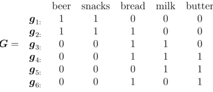
We use a toy transaction dataset to demonstrate how CBMF reveals underlying dominant patterns in the original data. Table 2.2 shows the toy dataset given by Koyut¨urk et al. [61], where each pattern in a row is a transaction in a shopper’s purchase history.

Table 2.2: Toy transaction dataset

beer snacks bread milk butter

g_1: 1 1 0 0 0 g_2: 1 1 1 0 0 G= g_3: 0 0 1 1 0 g_4: 0 0 1 1 1 g_5: 0 0 0 1 1 g_6: 0 0 1 0 1

(40)

A rank-2 binary matrix factorization for BMF (2.5) produces the following approxima-tion. U W u1 u2 w1: w2: G≈                 0 1 0 1 1 0 1 0 1 0 1 0                    0 0 1 1 1 1 1 1 0 0   

Virtual transaction Weight

w1:: {bread, milk, butter} 4

w2:: {beer, snacks, bread} 2

Each transaction in G is approximated by a virtual transaction w1: or w2:, and each

column of matrixU gives the weights of the corresponding virtual transactions. For example,

w1: has weight 4 because there are four 1s in u1, meaning that transactions g3: to g6: are

represented by, or assigned to w1:. Thus we call w1: or w2: pattern vector, which finds the

dominant patterns, and u1 or u2 presence vector, which shows how the original patterns

are represented by the pattern vectors. The constraint on the rows of U in BMF (2.5) guarantees that each original transaction is represented by at most one virtual transaction. We conclude that problem (2.5) reveals the dominant patterns in rows of the original data. Similarly, problem (2.4) reveals the dominant patterns in columns of the original data.

2.7.2

Pattern Extraction

In this section we compare the performance of CBMF for extracting patterns on two synthetic binary datasets with PROXIMUS and other popular approximation methods that work well on continuous data, including SVD, NMF, and k-means. We used embedded MATLAB

(41)

packages for SVD and k-means, and the MATLAB package developed by H. Kim and H. Park [56] for NMF. For each method, we compare the sparsity patterns of the original and the approximate matrix, tell whether the rank of the approximate matrix matches the number of clusters in the original matrix, and calculate the Frobenius norm of the approximation error, i.e., the square root of the objective value used in our CBMF model.

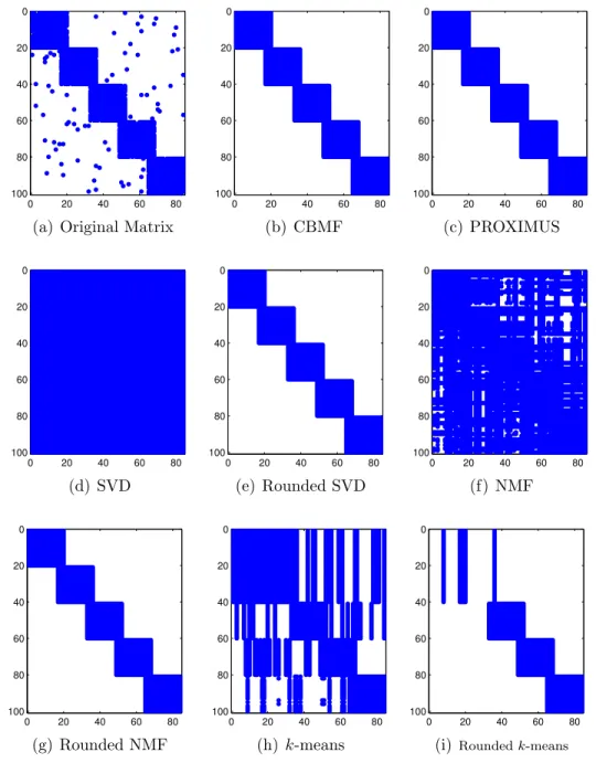
Two artificial datasets were generated by implanting uniform patterns into groups of rows on a background of uniform white noise. The first matrix of 100× 54, shown in Fig. 2.1(a), contains five overlapping uniform patterns, each of which is implanted into a cluster of 20 rows. Each entry of the matrix is set to 1 with probability 0.01 as the background noise. Let l denote the distance of two leading columns in successive patterns, and r denote the number of overlapping columns shared by two successive patterns. Each pattern has (l+r) columns. The (i, j)-th entry belonging to a row cluster containing the k-th pattern is set to 1 with probability 0.85, where (k−1)l+ 1≤j ≤kl+r. In our experiments, we set l = 16, and r = 4. Note that the rank of the approximate matrix obtained by each method is 5, which matches the number of patterns in the original matrix. Fig. 2.1 shows the sparsity patterns of the original matrix and the approximate matrix obtained by each method. It shows that SVD and NMF hardly reveal any underlying patterns, and k-means can reveal only a few patterns, as the approximate matrice generated by these three methods usually contain entries of negative values and non-binary values, which are hard to interpret. Thus we change the negative sign to positive and round each entry to generate binary approximate matrices. Fig. 2.1(e), 2.1(g), and 2.1(i) show that rounded SVD, rounded NMF, and rounded k-means successfully remove the background noise. In fact, Fig. 2.1 shows that CBMF, PROXIMUS, rounded SVD, and rounded NMF successfully extract the original patterns. The approximation error of all these four algorithms is 19.29. Thus for this dataset, CBMF has the same performance with the other three methods. However, for more complicated datasets, CBMF shows its superior performance over others, as will be discussed in the next example. In addition, the errors of SVD, NMF, k-means, and rounded k-means are 17.14,

(42)

17.22, 23.09, and 28.53, respectively. Though SVD and NMF have relatively small errors, the real-valued entries do not give much information about the underlying patterns.

0 20 40 60 80 0 20 40 60 80 100

(a) Original Matrix

0 20 40 60 80 0 20 40 60 80 100 (b) CBMF 0 20 40 60 80 0 20 40 60 80 100 (c) PROXIMUS 0 20 40 60 80 0 20 40 60 80 100 (d) SVD 0 20 40 60 80 0 20 40 60 80 100 (e) Rounded SVD 0 20 40 60 80 0 20 40 60 80 100 (f) NMF 0 20 40 60 80 0 20 40 60 80 100 (g) Rounded NMF 0 20 40 60 80 0 20 40 60 80 100 (h)k-means 0 20 40 60 80 0 20 40 60 80 100

(i)Roundedk-means

Figure 2.1: Pattern extraction for sample binary matrix with five overlapping patterns.

The second matrix of 250×84 also has five row clusters, but each cluster has two patterns randomly chosen from the five patterns generated in the first example. Fig. 2.2 shows the sparsity patterns of the original matrix and the approximate one obtained by each method. It shows that CBMF, rounded SVD, and rounded NMF all discover the underlying patterns

(43)

quite well, PROXIMUS reveals most of the underlying patterns, k-means and rounded k-means reveal some of the patterns, while SVD and NMF hardly reveal any patterns. In addition, the approximation of all methods except PROXIMUS and rounded SVD are of rank 5, which matches the number of clusters in the original dataset. PROXIMUS provides a rank-10 approximation. The redundancy in the approximation is the division of the second row cluster into several parts, which adds additional ranks for the approximation. Rounded SVD obtains an approximation rank of 7, because the quantization of each entry does not always preserve the rank of the matrix. The approximation error increases in the order SVD, NMF, PROXIMUS, rounded SVD, CBMF, rounded NMF, k-means, and rounded k-means, with values 34.75, 35.00, 38.91, 39.06, 39.09, 39.09, 39.82, and 46.20, respectively.

We conclude that CBMF works quite well for extracting patterns in binary datasets, and the approximation rank matches the number of clusters in the original datasets. PROXIMUS and rounded SVD are capable of revealing underlying patterns, but usually with a high rank approximation. Though SVD has the smallest approximation error, it is not suitable for binary datasets because the real-valued entries do not reveal much information about the binary patterns. For the same reason, the methods that work well for continuous data, such as NMF, do not work well for binary data. Note that rounded NMF has the same performance as CBMF for extracting underlying patterns with the same approximation rank and error, however, as discussed earlier, its storage space, the non-uniqueness of its solution, and the extra work for converting non-binary entries to binary ones rule it out for binary data. K-means and rounded k-means discover only some of the patterns, with a relative high approximation error. However, CBMF works quite well. Though it is quite similar to k-means, the key difference is that the centers in CBMF are restricted to be binary vectors, which reasonably interpret the original data.

(44)

0 50 0 50 100 150 200 250

(a) Original matrix

0 50 0 50 100 150 200 250 (b) CBMF 0 50 0 50 100 150 200 250 (c) PROXIMUS 0 50 0 50 100 150 200 250 (d) SVD 0 50 0 50 100 150 200 250 (e) Rounded SVD 0 50 0 50 100 150 200 250 (f) NMF 0 50 0 50 100 150 200 250 (g) Rounded NMF 0 50 0 50 100 150 200 250 (h)k-means 0 50 0 50 100 150 200 250

(i) Roundedk-means

Figure 2.2: Pattern extraction for sample binary matrix with five row clusters, each of which contains a randomly chosen pair of five overlapping patterns.

2.7.3

Association Rule Mining

In this section, we apply binary matrix factorization algorithms to speed up the process of association rule mining, a popular method for discovering relations between variables in large databases. Association rules are employed in many application areas including transaction data mining, book recommendations and tag recommendations for videos or

(45)

Table 2.3: Real datasets

Dataset # rows # columns # nonzeros min rowsum max rowsum

Transaction 150 20 862 5 10

ImageTag 2000 81 11740 4 20

images. However, the cost for determining such relations is usually quite high due to the large size of these datasets. We demonstrate how binary matrix factorization can reduce the cost by replacing the original dataset with a much smaller approximate dataset.

We showed a toy transaction matrix given by Koyut¨urk et al. [61] in Section 2.2. Each of the six transactions in G is approximated by two virtual transactions in W, and matrix

U gives the weights of the virtual transactions. Then we apply association rule mining algorithms to W instead of G. We can expect significant speedup in time for discovering association rules on large real datasets.

One real test dataset is a retail market basket data set [19] supplied by an anonymous Belgian retail supermarket. The other is the NUS-Wide flickr dataset [27] created by crawling photos from flickr and choosing tags for photos. Each row is an image and each column is a tag. If an image has a tag then the corresponding entry is 1, else 0. We filtered the datasets so that each row has at least two 1s, as the original datasets are very sparse. Table 2.3 describes the features of the filtered data.

2.7.3.1 Evaluation of Approximate Datasets

The key issue is how well the approximate datasets represent the original datasets. We use two measures to assess this. One is the objective value defined in the our CBMF model. In addition, we define another measure named Match Score, which tells how well the weighted patterns capture the original patterns. First we define a function as follows:

Match(S, z) =X s∈S

matched ones(s, z)

(46)

where S is a set of binary vectors, z is a binary vector, sum(s) is the number of ones in the binary vector s, and matched ones(s, z) is the number of matched ones between two binary vectors s and z. Now we define Match Score as follows:

Match Score = k X

i=1

Match(Si, wi:),

where Si is the set of rows in G that are approximated by wi:. For example, in the toy

example we have S 1 = {g3:, g4:, g5:, g6:}, S 2 = {g1:, g2:}, and thus Match Score = 2₂ + 3₃ + 2 2 + 2 2 + 2 2 + 3 3 = 6.

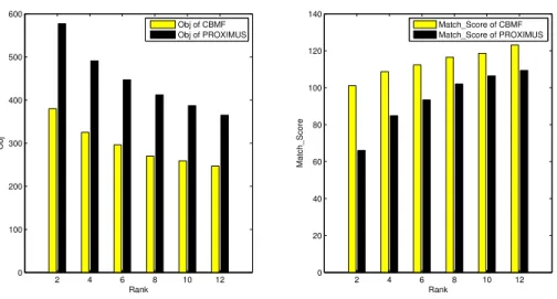
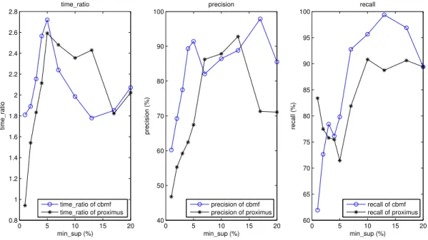
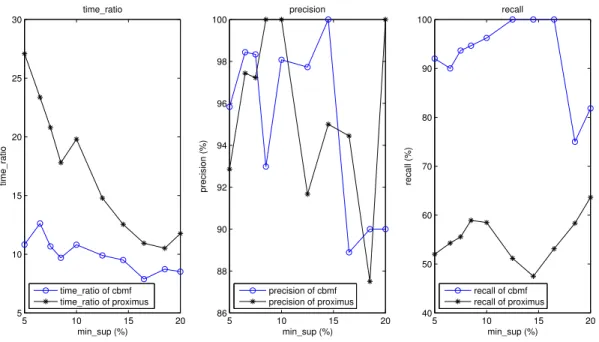
Note that a smaller objective value and a larger value of Match Score mean a better approximation to the original datasets. We then decompose the Transaction dataset by CBMF and PROXIMUS, and show the performance for different values of k in Fig. 2.3. However, PROXIMUS does not take k as an input parameter. Thus we apply the rule proposed in [70] to find the best solution of rank k among all patterns returned by PROX-IMUS. Fig. 2.3 shows that the objective value becomes smaller and the Match Score becomes larger as k becomes larger for both CBMF and PROXIMUS. This is in accordance with the fact that the approximate matrix should be closer to the original one as k becomes larger. Fig. 2.3 also shows that CBMF obtains a smaller objective value and a larger Match Score than PROXIMUS for each value of the rank, meaning that CBMF usually generates a better approximation to the original dataset than PROXIMUS does.

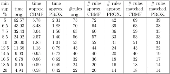
2.7.3.2 Evaluation of Association Rules

We further compare the association rules mined on the original datasets, and the approximate ones obtained by CBMF or PROXIMUS. We use an efficient MATLAB implementation of the well-known a-priori algorithm [12], named ARMADA [1], as the benchmark algorithm for association rule mining. We extended ARMADA so that it can accept any support value from 0 to 100, which is not restricted to only integers ≥ l, when specified as a percentage

(47)

2 4 6 8 10 12 0 100 200 300 400 500 600 Rank Obj Obj of CBMF Obj of PROXIMUS 2 4 6 8 10 12 0 20 40 60 80 100 120 140 Rank Match_Score Match_Score of CBMF Match_Score of PROXIMUS

F