Camdoop: Exploiting In-network Aggregation for Big Data Applications
Paolo Costa
†‡Austin Donnelly
†Antony Rowstron
†Greg O’Shea
††
Microsoft Research Cambridge
‡Imperial College London
Abstract
Large companies like Facebook, Google, and Microsoft as well as a number of small and medium enterprises daily process massive amounts of data in batch jobs and in real time applications. This generates high network traffic, which is hard to support using traditional, oversubscribed, network infrastructures. To address this issue, several novel network topologies have been proposed, aiming at increasing the bandwidth available in enterprise clusters.
We observe that in many of the commonly used work-loads, data is aggregated during the process and the output size is a fraction of the input size. This motivated us to ex-plore a different point in the design space. Instead of in-creasing the bandwidth, we focus on dein-creasing the traffic by pushing aggregation from the edge into the network.
We built Camdoop, a MapReduce-like system running on CamCube, a cluster design that uses a direct-connect network topology with servers directly linked to other servers. Camdoop exploits the property that CamCube servers forward traffic to perform in-network aggrega-tion of data during the shuffle phase. Camdoop supports the same functions used in MapReduce and is compati-ble with existing MapReduce applications. We demon-strate that, in common cases, Camdoop significantly re-duces the network traffic and provides high performance increase over a version of Camdoop running over a switch and against two production systems, Hadoop and Dryad/DryadLINQ.
1
Introduction
“Big Data” generally refers to a heterogeneous class of business applications that operate on large amounts of data. These include traditional batch-oriented jobs such as data mining, building search indices and log collection and analysis [2, 5, 41], as well as real time stream process-ing, web search and advertisement selection [3, 4, 7, 17].
To achieve high scalability, these applications usually adopt thepartition/aggregatemodel [13]. In this model, which underpins systems like MapReduce [1, 21] and Dryad/DryadLINQ [30, 48], there is a large input data set
distributed over many servers. Each server processes its share of the data, and generates a local intermediate result. The set of intermediate results contained on all the servers is then aggregated to generate the final result. Often the intermediate data is large so it is divided across multiple servers which perform aggregation on a subset of the data to generate the final result. If there areN servers in the cluster, then using allNservers to perform the aggregation provides the highest parallelism and it is often the default choice. In some cases there is less choice. For instance, selecting the topkitems of a collection requires that the final results be generated by a single server. Another ex-ample is a distributed user query, which requires the result at a single server to enable low latency responses [7, 13].
The aggregation comprises a shufflephase, where the intermediate data is transferred between the servers, and areducephase where that data is then locally aggregated on the servers. In the common configuration where all servers participate in the reduce phase, the shuffle phase has an all-to-all traffic pattern withO(N2)flows. This is challenging for current, oversubscribed, data center clus-ters. A bandwidth oversubscription of 1:xmeans that the bisection bandwidth of the data center is reduced by a fac-torx, so the data transfer rate during the shuffle phase is constrained. In current data center clusters, an oversub-scription ratio of 1:5 between the rack and the aggregation switch is often the norm [14]. At core routers oversub-scription is normally much higher, 1:20 is not unusual [15] and can be as high as 1:240 [26]. If few servers (possibly just one) participate in the reduce phase, the servers’ net-work links are the bottleneck. Further, the small buffers on commodity top-of-rack switches combined with the large number of correlated flows cause TCP throughput collaps-ing as buffers are overrun (theincastproblem) [13,44,45]. These issues have led to proposals for new network topologies for data center clusters [11, 26, 27, 40], which aim at increasing the bandwidth available by removing network oversubscription. However, these approaches only partly mitigate the problem. Fate sharing of links means that the full bisection bandwidth cannot be easily
achieved [12]. If the number of servers participating in the reduce phase is small, having more bandwidth in the core of the network does not help since the server links are the bottleneck. Finally, non-oversubscribed designs largely increase wiring complexity and overall costs [31]. In this paper, we follow a different approach to increase network performance: we reduce the amount of traffic in the shuffle phase. Systems like MapReduce already ex-ploit the fact that most reduce functions are commuta-tive and associacommuta-tive, and allow aggregation of intermediate data generated at a server using acombinerfunction [21]. It has also been shown that in oversubscribed clusters, per-formance can be further improved by performing a second stage of partial aggregation at a rack-level [47]. However, in [47] it is shown that at scale performing rack-level ag-gregation has a small impact on performance. One of the reasons is that the network link of the aggregating server is fair-shared across all the other servers in the rack and becomes a bottleneck.
We have been exploring the benefit of pushing aggrega-tion into the core network, rather than performing it just at the edge. According to [21], the average final output size in Google jobs is 40.3% of the intermediate data set sizes. In the Facebook and Yahoo jobs analyzed in [18], the re-duction in size between the intermediate and the output data is even more pronounced: in 81.7% of the Facebook jobs with a reduce phase, the final output data size is only 5.4% of the intermediate data size (resp. 8.2% in 90.5% of the Yahoo jobs). This demonstrates that there is opportu-nity to aggregate data during the shuffle phase and, hence, to significantly reduce the traffic.
We use a platform called CamCube [9,20], which, rather than using dedicated switches, distributes the switch func-tionality across the servers. It uses a direct-connect topol-ogy with servers directly connected to other servers. It has the property that, at each hop, packets can be intercepted and modified, making it an ideal platform to experiment with moving functionality into the network.
We have implemented Camdoop, a MapReduce-like system running on CamCube that supports full on-path aggregation of data streams. Camdoop builds aggrega-tion trees with the sources of the intermediate data as the children and roots at the servers executing the final reduc-tion. Aconvergecast[46] is performed, where all on-path servers aggregate the data (using a combiner function) as it is forwarded towards the root. Depending on how many keys are in common across the servers’ intermediate data sets, this reduces network traffic because, at each hop, only a fraction of the data received is forwarded.
This has several benefits beyond simply reducing the data being transferred. It enables the number of reduce tasks to be a function of the expected output data size, rather than a function of theintermediatedata set size, as is normally the case. All servers that forward traffic will effectively participate in the reduce phase, distributing the
computational load. This is important in workloads where the output size is often much smaller than the intermedi-ate data size (e.g., in distributed log data aggregation) or where there is a requirement to generate the result at a single server (e.g., in atop-kjob).
We present a detailed description of Camdoop, and demonstrate that it can provide significant performance gains, up to two orders of magnitude, when associative and commutative reduce functions are used and common keys exist across the intermediate data. We describe how Camdoop handles server failures, and how we ensure that each entry in the intermediate data is included exactly once in the final output in the presence of failures. We also show that even when the reduce function is not as-sociative and commutative, on-path aggregation still pro-vides benefits: Camdoop distributes the sort load across all servers and enables parallelizing the shuffle with the reduce phase, which further reduces the total job time. Fi-nally, Camdoop leverages a custom transport layer that by exploiting application-level knowledge allows a content-based priority scheduling of packets. Even when aggrega-tion is not performed, this helps ensure that reduce tasks are less likely to stall because of lack of data to process.
Camdoop supports the same set of functions originally used in MapReduce [21] and then in Hadoop [1]. It is designed to be a plug-in replacement for Hadoop and be compatible with the existing MapReduce jobs. We chose MapReduce as the programming model due to its wide applicability and popularity. However, our approach could also be extended to other platforms that use a parti-tion/aggregate model, e.g., Dryad [30] or Storm [7].
2
MapReduce
A MapReduce program consists of four functions: map,
reduce,combiner, andpartition. The input data is
split intoC chunks and, assuming N servers, approxi-matelyC/Nchunks are stored per server. Usually a chunk is no larger thanSMB, e.g.S=64, to increase parallelism and improve performance if tasks need be rerun.
Each job comprisesMmaptasks, where normallyM=C
andCN. These execute locally on each server process-ing a chunk of input data. Each map task produces an in-termediate data set consisting of (key, value) pairs, stored on the server, sorted by key. If the thereducefunction is associative and commutative, acombinerfunction can be used to locally aggregate the set of intermediate results generated by a map task. Thecombinerfunction often just coincides with thereducefunction.
The intermediate data is then processed byR reduce
tasks. Each task is responsible for a unique range of keys. For each key, it takes the set of all values associated with that key and outputs a (key, values) pair. Each server can run one or more reduce tasks. The reduce tasks require all the intermediate data consisting of all keys (with the asso-ciated values) they are responsible for. Hence, each server
2
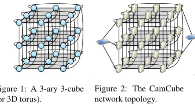
Figure 1: A 3-ary 3-cube (or 3D torus).
1
Figure 2: The CamCube network topology.
takes the sorted local intermediate data and splits it intoR
blocks, with each block containing all keys in a range re-quired by a single reduce task. The blocks are transferred to the server running the reduce task responsible in the
shuffle phase. IfR≥N then an all-to-all traffic pattern is generated, with each server sending 1/Nth of the locally stored intermediate data toN−1 servers.
Thepartitionfunction encodes how the key ranges
are split across the reduce tasks. Often, just a default hash-ing function is used. However, if some additional prop-erties are required (e.g., ensuring that concatenating the output files produced by the reduce tasks generates a cor-rect total ordering of keys), a more complexpartition
function can be used.
The parameterM is simply a function of the input data size and the number of servers N. However, setting the valueRis a little more complex and it can have significant performance impact. Rhas to be set as a function of the
intermediatedata set size, because 1/Rth of the interme-diate data set is processed by each reduce task. Obviously, the input data set size is fixed and, provided all the func-tions are deterministic, the output data set size will simply be a function of the input data set size. However, the in-termediate data set size is a function of the input data set size,N,M, and the ratio of input data to output data for
themapandcombinerfunctions.
In some scenarios, for example in web search queries or
top-kjobs, there is a need to have R=1. In others, for example in multi-round MapReduce jobs, storing the out-put on a smaller set of servers can be beneficial. Camdoop enables selectingRbased on the output data set size, but still allowsallservers to contribute resources to perform the aggregation, even whenR=1.
3
CamCube overview
CamCube [9, 20] is a prototype cluster designed using commodity hardware to experiment with alternative ap-proaches to implementing services running in data cen-ters. CamCube uses a direct-connect topology, in which servers are directly connected to each other using 1 Gbps Ethernet cross-over cables, creating a 3D torus [37] (also known as a k-ary 3-cube), like the one shown in Figure 1. This topology, popular in high performance computing,
e.g. IBM BlueGene/L and Cray XT3/Red Storm, provides multiple paths between any source and destination, mak-ing it resilient to both link and server failure, and efficient wiring using only short cables is possible [10]. Figure 2 shows an example of a CamCube with 27 servers. Servers are responsible for routing all the intra-CamCube traffic through the direct-connect network. Switches are only used to connect CamCube servers to the external networks but are not used to route internal traffic. Therefore, not all servers need be connected to the switch-based network, as shown in Figure 2.
CamCube uses a novel networking stack, which sup-ports a key-based routing functionality, inspired by the one used in structured overlays. Each server is automat-ically assigned a 3D coordinate(x,y,z), which is used as the address of the server. This defines a 3D coordinate space similar to the one used in the Content-addressable Network (CAN) [38], and the key-space management ser-vice exploits the fact that the physical topology is the same as the virtual topology. In CamCube, keys are encoded us-ing 160-bit identifiers and each server is responsible for a subset of them. Keys are assigned to servers as follows. The most significantkbits are used to generate an(x,y,z)
coordinate. If the server with this coordinate is reachable, then the identifier is mapped to this server. If the server is unreachable, the identifier is mapped to one of its neigh-bors. The remaining(160−k)bits are used to determine the coordinate of this neighbor, or of another server if all neighbors also failed. This deterministic mapping is con-sistent across all servers, and handles cascading failures.
The main benefit of CamCube is that by using a direct-connect topology and letting servers handle packet for-warding, it completely removes the distinction between the logical and the physical network. This enables ser-vices to easily implement custom-routing protocols (e.g., multicast or anycast) as well as efficient in-network ser-vices (e.g., caching or in-network aggregation), without incurring the typical overhead (path stretch, link sharing, etc.) and development complexity introduced by overlays. The CamCube software stack comprises a kernel driver to send and receive raw Ethernet frames. In our prototype, the packets are transferred to a user-space runtime, written in C#. The runtime implements the CamCube API, which provides low-level functionality to send and receive pack-ets to/from the six one-hop physical neighbors. All further functionality, such as key-based routing and failure detec-tion as well as higher-level services (e.g., a key-value store or a graph-processing engine) are implemented in user-space on top of the runtime. The runtime manages the transmission of packets and each service is provided with a service-specific queue for outbound packets. The run-time polls these queues in a round-robin fashion, achiev-ing fair sharachiev-ing of the outbound links across the services.
Experiments with our prototype show that the overhead of distributing the routing across the servers and of
mak-ing them participate in packet forwardmak-ing is tolerable: servers are able to sustain 12 Gpbs of throughput (i.e., all 6 links running at full capacity) using 21% of the CPU [20].
To fully achieve the performance benefits of CamCube, services should be designed so as to exploit the network topology and server forwarding. For instance, Camdoop obtains high performance by adopting a custom routing and transport protocol, and performing in-network aggre-gation. Yet, legacy applications can still benefit from CamCube due to its high bisection bandwidth. We im-plemented a TCP/IP service, which enables running un-modified TCP/IP applications on CamCube. To evaluate the performance that these applications could achieve in CamCube, we ran an experiment on our 27-server testbed (described in Section 5) in which every server simulta-neously transferred 1 GB of data to each of the other 26 servers using TCP. This creates an all-to-all traffic pattern. We obtained a median aggregate TCP inbound through-put of 1.49 Gbps per server, which is higher than the maximum throughput achievable in a conventional cluster where servers have 1 Gbps uplinks to the switch. We also measured the average RTT, using a simple ping service, obtaining a value of 0.13 ms per each hop. In an 8x8x8 CamCube (512 servers), this would lead to aworst-case
RTT of 1.56 ms (the average-case would be 0.78 ms).
4
Camdoop
Camdoop is a CamCube service to run MapReduce-like jobs. It exploits the ability of custom forwarding and pro-cessing of packets on path to perform in-network aggrega-tion, which improves the performance of the shuffle and reduce phase. An instance of the Camdoop service runs on all CamCube servers. Any CamCube server connected to the switch-based network can act as a front-end and re-ceive jobs from servers external to the CamCube. A job description includes ajobId, the code for map, reduce and any other functions required, such as the combiner and partition function, as well as a description of the input data and other runtime data such as the value ofR. Camdoop assumes that all the functions are deterministic, which is the normal case in MapReduce jobs. The input data set is stored in a distributed file system implemented on top of a key-value store running on CamCube, as with GFS [25] or HDFS [1]. It is split into multiple chunks, each with a 160-bit identifier (chunkId). When a data set is inserted, the chunkIds are generated to ensure that chunks are, ap-proximately, uniformly distributed. The chunkId deter-mines the servers that will store a file replica (by default a chunk is replicated three times). The final output can be written to local disk, inserted into the distributed file sys-tem or inserted as key-value pairs into a key-value store. If the distributed file system is used, at job submission, the identifiers of the chunks comprising the output file can be generated so the server running the reduce task would be the primary replica for these chunks. This is done by
setting the topkbits of the chunk identifiers to be the co-ordinate of the desired server. Without failures, the two replicas are stored on one-hop neighbors of the primary replica and a different network link is used for each one.
When a job request is received by a front-end server, it is broadcast to all the other servers using the intra-CamCube network. When a server receives the broadcast request it determines if, for any of the input chunks, it is the primary replica and if so initiates a map task to process the locally stored file. However, any server can run a map task on any file, even though it is not storing a replica of the file. This is required, for example, to handle stragglers. The intermediate data generated by the map task is not stored in the distributed store but is sorted and written to a lo-cal disk, as with MapReduce and Hadoop. Each output is tagged with a 160-bit identifier,mapTaskId, that is equal to the chunkId of the input chunk processed by that task. If multiple map tasks run on the same server then multi-ple intermediate data files will be produced, each with a different mapTaskId. Once all the intermediate data has been written to disk the map phase has completed, and the shuffle and reduce phase commences. Camdoop sup-ports both a synchronous start of the shuffle phase using an explicit message from a controller (to perform cluster wide scheduling) but also allows servers to independently asynchronously initiate the shuffle phase.
4.1
On-path aggregation
Camdoop pushes aggregation into the network and par-allelizes the shuffle and reduce phases. To achieve this, it uses a custom transport service that provides reliable communication, application-specific scheduling of pack-ets and packet aggregation across streams.
Conceptually, for each reduce task, the transport service forms a spanning tree that connects all servers, with the root being the server running the reduce task. This is similar to how overlay trees are used for performing con-vergecast [46]. This is hard to implement in traditional switched-based networks because servers have a single link to the switch; forwarding traffic through a server, even in the same rack, saturates the inbound link to the server [47]. It only makes sense when bandwidth over-subscription rates are very high.
We start by describing a simplified version of the pro-tocol used in Camdoop, assumingR=1 andnofailures, and then remove these assumptions.
Tree-building protocol Camdoop uses a tree topology similar to the one in Figure 3(a). In principle, any tree topology could be used but, for reasons that we will ex-plain later, this (perhaps surprising) topology maximizes network throughput and load distribution. The internal vertices are associated with a 160-bit identifier, called ver-texId. The leaves represent the outputs of the map tasks and are associated to the corresponding mapTaskId.
MapTaskId VertexId
(a) Logical view. (b) Physical view.
Figure 3: Logical and physical view of the tree topology used in Camdoop on a 3x3x3 CamCube.
is mapped to a different server, a different coordinate is used for the topkbits of each vertexId. For the remaining bits, a hash of the jobId is used. The vertexId of the server selected to run the reduce task is denoted asrootId.
Servers use the functiongetParentto compute the tree topology. It takes as input the rootId and an identifieri
(either a mapTaskId or a vertexId) and returns the iden-tifier of the parent ofi, or a null value ifi=rootId. To achieve high throughput, the implementation of this func-tion must ensure high locality. WhengetParent receives as input a mapTaskId, it looks at the coordinate generated from its topkbits and returns the vertexId that generates the same coordinate. Instead, when a vertexIdvis passed togetParent, it always returns a vertexIdpsuch that the coordinate ofvis a one-hop neighbor of the coordinate of
p in the 3D space. These conditions ensure that, in the absence of failures, map outputs are always read from the local disk (rather than from the network) and parents and children of the internal vertices are one-hop neighbors.
Figure 3(b) illustrates how the logical topology in Fig-ure 3(a) is mapped onto a 3x3x3 CamCube using the mechanism just described (mapTaskIds omitted for clar-ity). This can be trivially extended to handle larger scales.
Shuffle and reduce phase When a server receives the job specification, it locally computes the list of the vertex-Ids of the job and identifies the subset that are mapped to itself. In the absence of failures, exactly one vertexId is mapped to a server. Then, by using the above function it computes the identifiers of its parent and children.
During the shuffle phase, the leaves of the tree (i.e., the mapTaskIds) just greedily send the sorted intermediate data to their parent identifiers, using the CamCube key-based routing. Every internal vertex merges and aggre-gates the data received by its children. To perform this efficiently, per child, a small packet buffer is maintained with a pointer to the next value in the packet to be ag-gregated. When at least one packet is buffered from each child, the server starts aggregating the (key,value) pairs across the packets using the combiner function. The ag-gregate (key,value) pairs are then sent to the parent. At the root, the results are aggregated using the reduce function and the results stored.
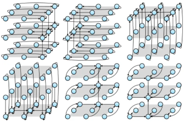
Figure 4: The six disjoint trees.
If a child and a parent identifier are mapped to the same physical server, a loopback fast-path is used. Otherwise, the transport service used in Camdoop provides a reliable in-order delivery of packets at the parent. Camdoop uses a window-based flow-control protocol and window update packets are sent between a parent and a child.
Load balancing and bandwidth utilization The de-scribed approach does not evenly distribute load across the tree, as some vertices have higher in-degree than oth-ers. Further, it is not able to exploit all six outbound links, as each server has only one parent to which it sends pack-ets over a single link. To address these issues, Camdoop creates six independentdisjoint spanning trees, all shar-ing the same root. The trees are constructed such that every vertexId, except the root, has a parent vertexId on a distinct one-hop server for each of the six trees. Con-ceptually, this can be achieved by taking the topology in Figure 3(b) and rotating it along theY andZ axis. The resulting trees are shown in Figure 4. This explains the choice of the topology used in Figure 3(a) as it enables the use of six disjoint trees.
This ensures that, except for the outbound links of the root (which are not used at all), each physical link is used by exactly one(parent, child)pair in each direction. This enables the on-path aggregation to potentially exploit the 6 Gbps of inbound and outbound bandwidth per server. It also improves load balancing; the resources contributed are more uniformly distributed across servers. The state shared across trees is minimal and they perform the aggre-gation in parallel, which further improves performance.
When using multiple trees, the intermediate data stored at each server is striped across the trees. This requires that
i)the keys remain ordered within each stripe and thatii)
the mapping between key and stripe be performed con-sistently across all servers, so that the same keys are al-ways forwarded through the same stripe. Camdoop ap-plies a hash function to the keys so as to roughly distribute them uniformly across the six stripes. In general, order-preserving hash functions cannot be used, because the key distribution might be skewed. Therefore, at the root, the six streams and the local map output need to be merged
to-gether to provide the final output. If the key distribution is known in advance, a more efficient solution is to split the keyspace in six partitions of equal size such that the order of the keys is preserved across partitions and assign each partition to a different tree. In this way, the root just needs to merge the stream of each tree with the local map out-put data (which would have also been partitioned accord-ingly) and then concatenate the resulting streams, without requiring a global merge. However, since this approach is not always applicable, in all the experiments presented in the next section, the hash-based approach is used.
A drawback of using six disjoint trees is that this in-creases the packet hop count compared to using a single shortest-path tree. As we will see in Section 5.2, when
R is very large and there is little opportunity for aggre-gating packets, this negatively impacts the performance. In the design of Camdoop, we preferred to optimize to-wards scenarios characterized by high aggregation and/or low number of reduce tasks and this motivates our choice of using six trees. However, if needed, a different tree topology could be employed to obtain different tradeoffs.
Multiple reduce tasks and multiple jobs HandlingR> 1 is straightforward: each reduce task is run indepen-dently, and hence six disjoint trees are createdper reduce task. This means that, in the absence of failures, each link is shared byRtrees, i.e., one per reduce task. Each tree uses a different packet queue and the CamCube queuing mechanism ensures fair sharing of the links across trees. The same mechanism is also used to handle multiple jobs. Each job uses a different set of queues and the bandwidth is fair-shared across jobs.
Packet queue sizes are controlled by an adaptive pro-tocol that evenly partitions the buffer space between the multiple reduce tasks and jobs. This ensures that the ag-gregate memory used by Camdoop to store packets is con-stant, regardless the number of tasks running. In the ex-periments presented in Section 5, the aggregate memory used by the packet queues was 440 MB per server.
4.2
Incorporating fault-tolerance
A key challenge in the design of on-path aggregation is to make it failure tolerant, and in particular to ensure that during failures we do not double count (key,value) pairs. We first describe how we handle link failures and then we discuss how we deal with server failures.
Handling link failures is easy. To route packets from children to parents, we use the CamCube key-based rout-ing service, which uses a simple link-state routrout-ing proto-col and shortest-paths. In case of link failures, it recom-putes the shortest path and reroutes packets along the new path. While this introduces a path stretch (parents and children may not be one-hop neighbors any longer), due to the redundancy of paths offered by the CamCube topol-ogy, this has low impact on performance, as we show in Section 5.4. Our reliable transmission layer recovers any
packets lost during the routing reconfiguration.
We now focus on server failures. The CamCube API guarantees that, in case of server failures, vertices are remapped to other servers in close proximity to the failed server. The API also notifies all servers that a server has crashed and that its vertex has been remapped. When the parent of the vertexvthat was mapped to the failed server receives the notification, it sends a control packet to the server that has now become responsible forv. This packet contains the last key received from the failed server. Next, each child ofvis instructed to re-send all the (key,value) pairs from the specified last key onwards. Since keys are ordered, this ensures that the aggregation function can proceed correctly. If the root of the tree fails, then all (key,value) pairs need to be re-sent, and the new vertex simply requests each child to resend from the start.
Of course, as in all implementations of MapReduce where the intermediate data is not replicated, if the failed server stored intermediate data, it will need to be regen-erated. Some of the children of the failed vertex repre-sent the map tasks that originally ran on the failed server, each identified by a different mapTaskId. On a failure, the CamCube API ensures that these identifiers are remapped to active servers. When these servers receive the control packet containing the last key processed by the parent of the failed vertex, they start a new map task using the map-TaskId to select the correct input chunk (recall that the chunkId is equal to the mapTaskId). If the distributed file system is used, the server to which the mapTaskId is remapped is also a secondary replica for that chunk. This ensures that, even in case of failure, the map tasks can read data locally. As the map function is deterministic, the sequence of keys generated would be the same as the one generated by the failed server, so the map task does not re-send (key,value) pairs before the last key known to have been incorporated.
4.3
Non commutative / associative functions
Although Camdoop has been designed to exploit on-path aggregation, it is also beneficial when aggregation cannot be used, i.e., when the reduce function is not commutative and associative (e.g., computing the median of a set of values). In these cases, Camdoop vertices only merge the streams received from their children, without performing any partial aggregation. Although this does not reduce the total amount of data routed, it distributes the sort load. In traditional MapReduce implementations, each reduce task receives and processesN−1 streams of data plus the locally stored data. In Camdoop, instead, each reduce task only merges 6 streams, and the local data. Even when
R<Nall servers participate in the merge process. Also, in Camdoop the computation of the reduction phase has been parallelized with the shuffle phase. Since all the streams are ordered by key, as soon as the root re-ceives at least one packet from each of its six children, it
can immediately start the reduce task without waiting for all packets. This also implies that there is no need to write to disk the intermediate data received by the reduce task, which further helps performance. Beside reducing over-all job time, maximizing concurrency between the shuf-fle and reduce phase helps pipelining performance where the final output is generated as the result of a sequence of MapReduce jobs. As the reduce tasks produce pairs, the next map function can be immediately applied to the generated pair.
5
Evaluation
We evaluate the performance of Camdoop using a proto-type 27-server CamCube and a packet-level simulator to demonstrate scaling properties.
Testbed The 27 servers form a 3x3x3 direct-connect net-work. Each server is a Dell Precision T3500 with a quad-core Intel Xeon 5520 2.27 GHz processor and 12 GB RAM, running an unmodified version of Windows Server 2008 R2. Each server has one 1 Gbps Intel PRO/1000 PT Quadport NIC and two 1 Gbps Intel PRO/1000 PT Dual-port NICs, in PCIe slots. We are upgrading the platform to use 6-port Silicom PE2G6i cards, but currently only have them in sample quantities, so in all our experiments we used the Intel cards. One port of the four port card is con-nected to a dedicated 48-port 1 Gbps NetGear GS748Tv3 switch (which uses store-and-forward as opposed to cut-through routing). Six of the remaining ports, two per mul-tiport NIC, are used for the direct-connect network.
The Intel NICs support jumbo Ethernet frames of 9,014 bytes (including the 14 byte Ethernet header). In Cam-Cube experiments we use jumbo frames and use default settings for all other parameters on the Ethernet cards, including interrupt moderation. We analyzed the perfor-mance of the switch using jumbo frames and found that the performance was significantly worse than using the traditional 1,514 byte Ethernet frames so all switch-based experiments use this size.
Each of the servers was equipped with a single stan-dard SATA disk, and during early experiments we found that the I/O throughput of the disk subsystem was the per-formance bottleneck. We therefore equipped each server with an Intel X25-E 32 GB Solid State Drive (SSD). These drives achieve significantly higher throughput than the mechanical disks. We used these disks to store all input, intermediate and output data used in the experiments.
Simulator Our codebase can be compiled to run either on the CamCube runtime or on a packet-level discrete event simulator. The simulator accurately models link proper-ties, using 1 Gbps links and jumbo frames. The simu-lator assumes no computation overhead. We ran simula-tions with 512 servers, representing an 8x8x8 CamCube. This is the same order of magnitude as the average num-ber of servers used per MapReduce job at Google, which are 157, 268 and 394 respectively for the three samples
reported in [21]. Also, anecdotally, the majority of or-ganizations using Hadoop use clusters smaller than a few hundred servers [5].
Baselines Compared to existing solutions, Camdoop dif-fers in two ways. First, it uses the CamCube direct-connect topology, running an application specific routing and transport protocol. Second, it exploits on-path ag-gregation to distribute the agag-gregation load and to reduce the traffic. To quantify these benefits separately, we im-plemented two variants of Camdoop,TCP Camdoopand
Camdoop (no agg.), which we use as baselines. Both vari-ants run the same code as Camdoop for the map and re-duce phase, including the ability to overlap the shuffle and reduce phase but they do not aggregate packets on path. The difference between the two baselines lies in the net-work infrastructure and protocols used. TCP Camdoop transfers packets over the switch using TCP/IP. The Cam-doop (no agg.) baseline, instead, runs on top of CamCube and it uses the same tree-based routing and transport pro-tocol used by Camdoop. It also partially sorts the streams of data on-path but it does not aggregate them.
By comparing the performance of Camdoop (no agg.) against TCP Camdoop, we can quantify the benefit of running over CamCube and using custom network pro-tocols. This also shows the benefits of Camdoop when on-path aggregation cannot be used as discussed in Sec-tion 4.3. The comparison between Camdoop and Cam-doop (no agg.) shows the impact of on-path aggregation.
In our experiments, across a wide range of workloads and configuration parameters, Camdoop significantly out-performed the other two implementations. To demon-strate that the performance of the switch-based imple-mentation is good, we also compared its performance against two production systems: Apache Hadoop [1] and Dryad/DryadLINQ [30, 48]. As we show next, all Cam-doop versions, including the one running over the switch, outperform them.
5.1
Sort and Wordcount
We evaluate all the three versions of Camdoop against Hadoop and Dryad/DryadLINQ running over the switch. We use two different jobs: Sort andWordcount, cho-sen as they are standard tutorial examples included in the Hadoop and DryadLINQ distributions and they are of-ten used to benchmark different MapReduce implemen-tations. For Sort, we used the ’Indy’ variant of the sort benchmark [6] in which the input data consists of ran-domly distributed records, comprising a 10 byte key and 90 bytes of data. Each key is unique and the aim of the Sort is to generate a set of output files such that concate-nating the files generates a total ordering of the records based on the key values. In Wordcount the aim is to count the frequency with which words appear in a data set
These represent very different workloads. In Sort the in-put, intermediate and output data sizes are the same: there
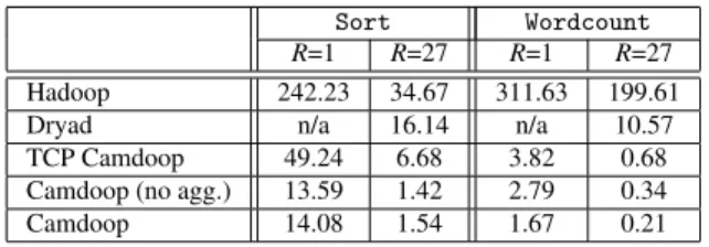
Sort Wordcount
R=1 R=27 R=1 R=27
Hadoop 242.23 34.67 311.63 199.61
Dryad n/a 16.14 n/a 10.57
TCP Camdoop 49.24 6.68 3.82 0.68 Camdoop (no agg.) 13.59 1.42 2.79 0.34 Camdoop 14.08 1.54 1.67 0.21
Table 1: Sort and Wordcount shuffle and reduce time (s).
is no aggregation of data across phases. In contrast, in Wordcount there is significant aggregation due to multiple occurrences of the same word in the original document corpus and in the intermediate data. From the statistics reported in [18, 21], we expect most workloads to have aggregation statistics closer to Wordcount.
We used Hadoop version 0.20.2 with default settings. We configured it so that all 27 servers could be used for map and reduce tasks, with one server running both the HDFS master and MapReduce job tracker. We increased the block size of HDFS to 128 MB because this yielded higher performance.
We used Dryad/DryadLINQ with default settings. DryadLINQ generates a Dryad dataflow graph which con-trols the number of instances of each type of process; therefore we could not vary this configuration parameters for the Dryad results. Further, in Dryad the master node cannot be used to run tasks. We therefore selected one server as the master and used the other 26 servers as work-ers. The impact of this is that there were fewer resources to be used to process the jobs. Therefore, to be conser-vative we automatically scaled the input data sets to be 26/27ths of the data set used for Camdoop and Hadoop. This effectively reduces the amount of work needed to be performed by Dryad by the load sustained on one server in the other implementations. In order to facilitate com-parisons, in all Camdoop-based implementations we write the results of the reduce task directly to the local disk and we use no replication in Hadoop and Dryad/DryadLINQ so that results are also written only to the local disk. In all experiments, we measure thejob time, which we define as the time from when the job is submitted to when the final results are stored on disk, and theshuffle and reduce time, which is the time from when all map tasks have com-pleted till the final results are stored on disk. The results in Table 1 show the shuffle and reduce time for all the imple-mentations usingR=1 andR=27 reduce tasks. For Dryad, we show only one result using the default data flow graph produced by DryadLINQ.
The Sort input data consists of 56,623,104 records. For Hadoop, these are randomly distributed in files stored in HDFS based on the block size. For Dryad and Camdoop we created files of approximately 200 MB and distributed them across the 27 servers (resp. 26 servers for Dryad). In this job, Camdoop and Camdoop (no agg.) demonstrate similar performance as there is no possibility to perform
aggregation. For TCP Camdoop the 1 Gbps link to the switch for the server running the reduce task is the bottle-neck and limits performance. When running withR=27, the TCP Camdoop version does not fully exploit the server bandwidth due to the overhead of managing multiple con-current TCP flows. We will demonstrate this in more de-tail later. The versions running on CamCube are able to exploit the higher bandwidth available, and therefore per-form better than TCP Camdoop but are constrained by the SSD disk bandwidth.
The results in Table 1 show that all Camdoop versions, including TCP Camdoop, outperform Hadoop and Dryad. Part of the performance gains is due to the design choices of Camdoop, most prominently the ability of overlapping the shuffle and the reduce phase (Section 4.3), which also reduces disk IO. We also finely optimized our implemen-tations to further improve the performance. In particular, Camdoop mostly utilizes unmanaged memory and stati-cally allocated packet buffers to reduce the pressure on the garbage collector, it exploits the support of C# for pointer operations to compare MapReduce keys eight bytes at a time rather than byte-by-byte, and, finally, it leverages an efficient, multi-threaded, binary merge-sort to aggre-gate streams. However, we also note that our versions are prototype implementations, omitting some functional-ity found in a full production system. This can also partly explain the difference in the results. Finally, we made no effort to tune Hadoop and Dryad but we used the default configurations. We show the data point simply to validate that the performance of TCP Camdoop is reasonable and we consider it as our main baseline.
For the Wordcount job the input data is the complete dump of the English language Wikipedia pages from 30th January 2010, and consists of 22.7 GB of uncompressed data. For Dryad and Camdoop implementations we split the file into 859 MB files and distributed one to each of the 27 servers (resp. 26 for Dryad). For Hadoop we stored these in HDFS using the modified block size. We also use map-side combiners in both Hadoop and Dryad. In this case, the intermediate data for the Wordcount can be ag-gregated. As in Sort, in Table 1 we show the shuffle and reduce time for all implementations, including the data points for Hadoop and Dryad to validate that the perfor-mance of TCP Camdoop is reasonable. In the Wordcount job the interesting comparison is between Camdoop and Camdoop (no agg.). Regardless the value ofR, Camdoop is usingallthe servers to help perform the aggregation, which results in less data and reduce overhead at the server running the reduce task. This yields a factor of 1.67 (R=1) and 1.62 (R=27) reduction in shuffle and reduce time.
5.2
Impact of aggregation
In order to conduct experiments across varying configu-ration parameters we created a synthetic job, inspired by the Wordcount example. We chose this type of job
1 10 100 1000 0 0.2 0.4 0.6 0.8 1 Tim e ( s) l ogsc ale Output ratio (S) TCP Camdoop Camdoop (no agg.) Camdoop
(a) R=1 reduce task.
1 10 100 1000 0 0.2 0.4 0.6 0.8 1 Tim e ( s) l ogsc ale Output ratio (S) Switch 1 Gbps (bound) Switch 6 Gbps (bound) Camdoop
(b) R=1 reduce task (bounds).
1 10 100 1000 0 0.2 0.4 0.6 0.8 1 Tim e ( s) l ogsc ale Output ratio (S) TCP Camdoop Camdoop (no agg.) Camdoop (c) R=27 reduce tasks. 1 10 100 1000 0 0.2 0.4 0.6 0.8 1 Tim e ( s) l ogsc ale Output ratio (S) Switch 1 Gbps (bound) Switch 6 Gbps (bound) Camdoop
(d) R=27 reduce tasks (bounds).
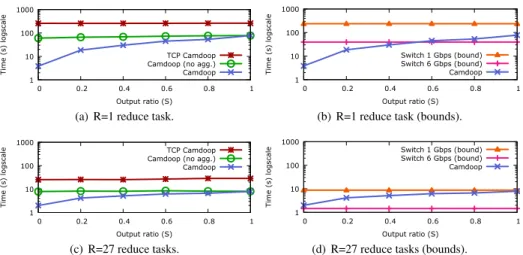
Figure 5: Varying the output ratio using R=1 and R=27 reduce tasks on the 27-server testbed (log-scale). cause, despite its simplicity, it is representative of many,
more complex, jobs in which aggregation functions typi-cally consist of simple additive or multiplicative integer or floating point operations, e.g., data mining or recommen-dation engines. The input data consists of 22.2 GB of data partitioned into 27 files, each 843 MB in size. The data consists of strings, generated randomly with a length uni-formly selected at random from 4 and 28 characters. The job uses a map function that takes each key and gener-ates a key value pair of (key, 1). There is no compression of input data to intermediate data, and the intermediate data will add a four-byte counter to each key. The reduc-tion funcreduc-tion sums the set of counts associated with a key, and can also be used as the combiner function. For ex-periments on the simulator, to allow us to scale, we use a smaller data set file size of 2 MB per server, which in our 512-server setup yields a total input data size of 1 GB.
To explore the parameter space we generate input data set files by specifying an output ratio,S. We defineS as the ratio of the output data set size to the intermediate data set size. If there areNinput files the lower bound onSis 1/Nand the maximum value isS=1. For clarity, we adopt the notation that S=0 means S=1/N. WhenS=1 there is no similarity between the input files, meaning that each key across all data files is unique, and there is no opportu-nity to perform on-path aggregation. Subsequently, at the end of the reduction phase the size of the output files will be the union of all keys in the input files, with each key assigned the value 1. For 27 servers this will result in an output data set size of approximately 28.3 GB (including the four-byte counters for each key). This represents the
worst-casefor Camdoop because no aggregation can be performed. WhenS=0 each key is common to all input files, meaning that the output file will be approximately 1.1 GB with each key having the value 27. This represents workloads where we can obtain maximum benefit from on path aggregation. As a point of comparison the Sort rep-resented a workload whereS=1, and the Wordcount
repre-sented a workload withS=0.56. A top-k query as used in search engines represents an example whereS=0 because all map tasks generate a sorted list ofkpairs and the out-put result is also a list ofkpairs. By varyingS, we are able to model different workloads, which result into different traffic savings and, hence, different performance gains.
In the results we do not consider the time taken by map tasks. Map times are independent of the shuffle and re-duce phase. They can vary significantly based on imple-mentation, and factors like the source of the input data, e.g. reading from an unstructured text data file as op-posed to reading from (semi-)structured sources, such as BigTable or using binary formats [22].
In the previous experiments the output data was stored to SSDs. Profiling Camdoop showed that for some data points the performance of reduce tasks was impacted by the SSD throughput by as much as a factor of two. We consider this a function of provisioning of the servers, and it would be very feasible to add a second SSD to increase the throughput so it would not impact performance. How-ever, as we were unable to do this, in these experiments we do not write the final output to disk. We do read all intermediate data from disk.
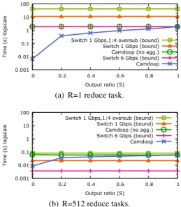
Impact of output ratio First we examine the impact of varying the output ratioSfromS=0 to 1 on the testbed and on the simulator. WhenS=0, full aggregation is possible, and whenS=1 no aggregation is possible. We use two val-ues ofR,R=1 andR=N, i.e., the lower and upper bounds onRassuming we have at most one reduce task per server. Figure 5 shows the shuffle and reduce time on the testbed as we varyS, using a log-scale y-axis. We com-pare Camdoop against Camdoop (no agg.) and TCP Cam-doop. Figure 5(a) shows the results for R=1 and Fig-ure 5(c) shows the results forR=27. In running the ex-periments for TCP Camdoop, we observed that the TCP throughput dropped for large values ofR. We were able to replicate the same behavior when generating all-to-all traffic using ttcp. Hence, this is not an artifact of our
TCP Camdoop implementation. We speculate that this is due to a combination of the small switch buffers [13] and the performance issues of TCP when many flows share the same bottleneck [34]. Potentially, this overhead could be partly reduced with a fine-tuned implementation and us-ing a high-end switch. For completeness, in Figure 5(b) and 5(d) we report thelower boundof the time that would be required by anyswitch-based implementation. This is computed by dividing the data size to be shuffled by the server link rate (1 Gbps). This therefore assumes full-bisection bandwidth and it does not include reduce time. As a further point of comparison, we also include the lower bound for a switch-based configuration withsix
1 Gbps links teamed together per server. Although the number of links per server is identical to CamCube, this configuration offers much higher bandwidth because in CamCube the server links are also used to forward traffic. Also, it would increase costs as it requires more switches and with higher fanout. We refer to the two lower bounds asSwitch (1 Gbps)andSwitch (6 Gbps).
The first important result in Figure 5(a) and 5(c) is the difference between TCP Camdoop and Camdoop (no agg.). Camdoop (no agg.) achieves significantly higher performance across all values of S, both for R=1 and
R=27. This is significant because it shows the base per-formance gain Camdoop achieves by using CamCube and a custom transport and routing protocol. In general, for Camdoop (no agg.) and TCP Camdoop the time taken is independent ofSsince the size of data transferred is con-stant across all values ofS.
We now turn our attention to the comparison of Cam-doop and CamCam-doop (no agg.). As expected, whenS=1 the performance of Camdoop and Camdoop (no agg.) is the same, because there is no opportunity to aggregate packets on-path. AsSdecreases, the benefit of aggrega-tion increases, reducing the number of packets forwarded, increasing the available bandwidth and reducing load at each reduce task. This is clearly seen in Figures 5(a) and Figure 5(c) for Camdoop forR=1 andR=27. WhenS=0, Camdoop achieves a speedup of 12.67 forR=1 and 3.93 forR=27 over Camdoop (no agg.) (resp. 67.5 and 15.71 over TCP Camdoop).
Figure 5(b) and 5(d) show that, at this scale, Camdoop
always achieves a lower shuffle and reduce time than Switch (1 Gbps). WhenR=1, for low values ofS Cam-doop also outperforms Switch (6 Gbps), but for large val-ues of S, Camdoop performance is bottlenecked on the rate at which the reduce task is able to process incoming data. In our implementation the throughput of the reduce code path varies approximately from 2.41 Gbps whenS=0 to 3.15 Gbps whenS=1). In a real implementation, the performance of Switch (6 Gbps) would suffer from the same constraint. WhenR=27, the shuffle and reduce time of Camdoop is always higher than Switch (6 Gbps) due to the lower bandwidth available in CamCube.
0.001 0.01 0.1 1 10 100 0 0.2 0.4 0.6 0.8 1 Tim e ( s) l ogsc ale Output ratio (S) Switch 1 Gbps,1:4 oversub (bound)
Switch 1 Gbps (bound) Camdoop (no agg.) Switch 6 Gbps (bound) Camdoop
(a) R=1 reduce task.
0.001 0.01 0.1 1 10 100 0 0.2 0.4 0.6 0.8 1 Tim e ( s) l ogsc ale Output ratio (S) Switch 1 Gbps,1:4 oversub (bound)
Switch 1 Gbps (bound) Camdoop (no agg.) Switch 6 Gbps (bound) Camdoop
(b) R=512 reduce tasks.
Figure 6: Varying the output ratio using R=1 and R=512 reduce tasks in the 512-server simulation (log-scale).
Figure 6 shows the simulation results. Due to the com-plexity of accurately simulating TCP at large scale, we only plot the values for the switch lower bounds. Building a full-bisection cluster at scale is expensive and most de-ployed clusters exhibit some degree of oversubscription, ranging from 1:4 up to 1:100 and higher. To account for this, we also compute the lower bound for a 512-server cluster assuming 40 servers per rack and 1:4 oversubscrip-tion between racks:Switch (1 Gbps, 1:4 oversub).
The simulated results confirm what we observed on the testbed. WhenR=1, Camdoopalwaysachieves the low-est shuffle and reduce time across allvalues of S. The simulation does not model computation time, which ex-plains why Camdoop outperforms Switch (6 Gbps) even for higher values of S. When R=512, Switch (6 Gbps) always yields the lowest time due to the higher bisec-tion bandwidth. More interesting is the comparison be-tween Camdoop and Switch (1 Gbps) whenR=512. Rout-ing packets usRout-ing six disjoint trees increases the path hop count, thus consuming more bandwidth. This explains why whenR=512, for most values ofS, Switch (1 Gbps) performs better than Camdoop. Using a single shortest-path tree would enable Camdoop, in this scenario, to achieve higher performance than Switch (1 Gbps) across all values ofS. As discussed in Section 4.1, we decided to optimize Camdoop for scenarios with lowRor lowS. However, even with this suboptimal configuration, Cam-doop is always better than Switch (1 Gbps, 1:4 oversub).
Impact of the number of reduce tasks In the previous experiment we discussed the impact of varyingS when
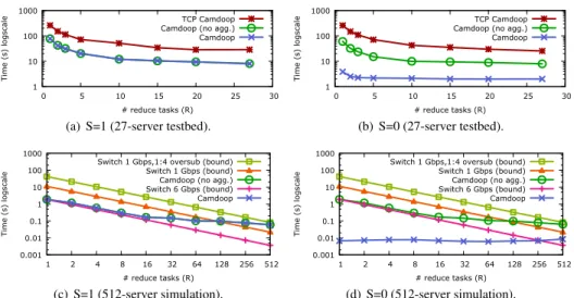
R=1 andR=N. In Figure 7, instead, we show the shuffle and reduce time on the testbed and on the simulator as we vary the number of reduce tasks, with and without aggre-gation. In these experiments, we used two data sets with
1 10 100 1000 0 5 10 15 20 25 30 Tim e ( s) l ogsc ale # reduce tasks (R) TCP Camdoop Camdoop (no agg.) Camdoop
(a) S=1 (27-server testbed).
1 10 100 1000 0 5 10 15 20 25 30 Tim e ( s) l ogsc ale # reduce tasks (R) TCP Camdoop Camdoop (no agg.) Camdoop (b) S=0 (27-server testbed). 0.001 0.01 0.1 1 10 100 1000 1 2 4 8 16 32 64 128 256 512 Tim e ( s) l ogsc ale # reduce tasks (R) Switch 1 Gbps,1:4 oversub (bound)
Switch 1 Gbps (bound) Camdoop (no agg.) Switch 6 Gbps (bound) Camdoop (c) S=1 (512-server simulation). 0.001 0.01 0.1 1 10 100 1000 1 2 4 8 16 32 64 128 256 512 Tim e ( s) l ogsc ale # reduce tasks (R) Switch 1 Gbps,1:4 oversub (bound)
Switch 1 Gbps (bound) Camdoop (no agg.) Switch 6 Gbps (bound) Camdoop
(d) S=0 (512-server simulation).
Figure 7: Varying the number of reduce tasks using S=0 and S=1 workloads (log-scale).
S=0 andS=1, representing the two ends of the spectrum for potential aggregation.
As already shown in the previous experiments, in Fig-ure 7(a) whenS=1 the performance of Camdoop and Cam-doop (no agg.) is the same. They both benefit from higher values ofR, as expected since the size of data received and processed by each reduce task decreases. They also outperform TCP Camdoop across all values ofR due to the higher bandwidth provided by CamCube and the cus-tom network protocols used. Similar trends are also visi-ble in the simulation results forS=1 in Figure 7(c). Cam-doop and CamCam-doop (no agg.) always outperform Switch (1 Gbps, 1:4 oversub) for all values ofR. They also exhibit higher performance than Switch (1 Gbps) for most values ofR, although for the reasons discussed above, with high values ofRandS, using six trees is less beneficial.
Figure 7(b) shows the results forS=0. We already ob-served that the performance of Camdoop (no agg.) and TCP Camdoop is generally unaffected by the value ofS
while Camdoop significantly improves performance when
S=0. However, the important observation here is that in this configuration the shuffle and reduce time for Cam-doop is largely independent of Ras shown in both Fig-ure 7(b) and 7(d). This is because, regardless the value of R, allservers participate in aggregation and the load is evenly distributed. This can be observed by looking at the distribution of bytes aggregated by each server. For instance, whenR=1, the minimum and maximum values of the distribution are within the 1% of the median value. This means that the shuffle and reduce time becomes a function of the output data size rather than the value ofR.
Rjust specifies the number of servers that store the final output. This is significant because it allows us to generate onlyfewoutput files (possibly just one) while still utiliz-ingallresources in the cluster. This property is important for multi-stage jobs and real time user queries.
The reason why in Figure 7(b) the shuffle and reduce time of Camdoop in the testbed withR=1 is higher than forR>1 is because the performance is bottlenecked by the computation rate of the reduce task. WhenRis higher, the size of the data aggregated by each reduce task is lower and, hence, the reduce task is not the bottleneck anymore. This effect is not visible in the simulation results because the simulator does not model computation time.
Finally, we note that in the simulation results in Fig-ure 7(d), Camdoop outperforms even Switch (6 Gbps) for most values ofR. This demonstrates that although Cam-Cube provides less bandwidth than Switch (6 Gbps), by leveraging on-path aggregation, Camdoop is able to de-crease the network traffic and, hence, to better use the bandwidth available and reduce the shuffle time.
The results show the benefits of using CamCube instead of a switch and also the benefits of on-path aggregation. We have so far shown results for experiments where only one job was running. However, often users run multiple jobs concurrently. In the next set of experiments we eval-uate the performance of Camdoop with such workloads.
5.3
Partitioning
The next experiment evaluates the impact of running mul-tiple jobs. We examine how this scales when using two different strategies for running multiple jobs,horizontal
andverticalpartitioning. In horizontal partitioning, we run multiple jobs by co-locating them. Hence, all servers run an instance of the map task for each job. In vertical partitioning, we divide the set of servers into disjoint parti-tions and run only the map tasks of any job on the servers assigned to it. In the horizontal partitioning, we run be-tween 1 andN reduce tasks, but the tasks are scheduled such to minimize the load skew across all servers. In ver-tical partitioning reduce tasks are only scheduled on the servers assigned to that job. Note that in vertical partition-ing servers in each partition contribute resources to both
0 0.5 1 1.5 2 2.5 R=1 R=27 R=1 R=13 Horizontal Vertical Time norm aliz ed to single job Job #1 Job #2
Figure 8: Effect of running multiple jobs. 1 1.2 1.4 1.6 1.8 2 R=1 (random) R=1 (neighbor) R=1 (root) R=27 (random) Time (normaliz ed ) Failure after 0.25T Failure after 0.5T Failure after 0.75T
Figure 9: Increase in shuffle and re-duce time caused by server failure.
0 20 40 60 20 KB 200 KB Time (m s)
Input data size / server TCP Camdoop
Camdoop (no agg) Camdoop
Figure 10: Shuffle and reduce time for small input data sizes.
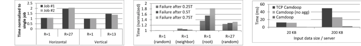
jobs, asallservers forward and aggregate packets on-path. Our experiments run two identical jobs concurrently. We start both jobs at the same time and we useS=1, which is the worst case. For horizontal partitioning we setR=1 andR=27, and have all servers run instances of the map task. In vertical partitioning we randomly assign thirteen servers to each job, leaving one server unassigned.
Figure 8 shows thenormalizedshuffle and reduce time for multiple jobs using horizontal and vertical partition-ing. For horizontal partitioning the values are normalized with respect to running a single job on all 27 servers with
R=1 orR=27, as appropriate. For vertical partitioning the values are normalized with respect to running a single job on 13 servers withR=1 orR=13, as appropriate.
The first important observation is that in all configura-tions, the time taken by the two jobs is approximately the same. This demonstrates the ability of CamCube to fair-share the bandwidth between two jobs by using separate outbound packet queues, as described in Section 4.1.
The results for horizontal partitioning in Figure 8 show that when R=1 the time taken for two jobs is approxi-mately at most 1.07 times longer than to complete asingle
job. WhenR=1 the bottleneck is the rate at which the re-duce task is able to process incoming data. In our testbed, the reduce code path can sustain a throughput of approxi-mately 3.15 Gbps. The available bandwidth is 6 Gbps, and hence, in general, the CamCube links are under-utilized. The links into the server running the reduce task have the highest utilization rate at 50.8%. Running multiple jobs allows the extra capacity to be utilized, and explains why the time to run two jobs is only less than 1.1 times longer than running a single job. In contrast, whenR=27, all links are fully utilized. Adding the second job causes the time to double because the links need be shared between jobs.
When using vertical partitioning andR=1, the two jobs take approximately as long as running a single job using 13 servers, as expected because the single experiment uses 50% of the CamCube resources. WhenR=13, intuitively you would expect the same, with the two jobs executing in the same time as the single task. However, in this case whereR=13 there is higher link utilization, and adding a second job increases job time up to a factor of 1.47.
The non-normalized figures show that the maximum time for two jobs whenR=13 is comparable to one job withR=27, as would be expected. This demonstrates that there is no performance difference between running jobs
horizontally or vertically partitioned. The achieved results are simply a function of the intermediate data set size and number of reduce tasks. This is important, because we envisage in many scenarios where the input data is stored in a key-value store that distributes input records across all servers in the CamCube cluster. Hence, running with horizontal partitioning will likely be the norm.
5.4
Failures
We now consider the impact of server failures on the per-formance of Camdoop. Camdoop uses a tree mapped onto the CamCube which, without failures, ensures that an edge in the tree is a single one-hop link in the Cam-Cube and each vertex is mapped to a different server. The failure of a server breaks this assumption. A single edge in the tree becomes a multi-hop path in the CamCube. Also, the load on other servers increases as they need to perform the aggregation on behalf of the failed server. This persists until the server is replaced, assuming it is replaced. Also, if the failure occurs during the shuffle phase, data that has been lost needs to be re-sent.
In this experiment, we want to measure the efficiency of the recovery protocol detailed in Section 4.2 and the increase in the job execution time due to a server fail-ing durfail-ing the shuffle phase. We test this on the testbed as the simulator does not model computational overhead. We fail a server after the shuffle phase has started and re-port the total shuffle and reduce time (including the time elapsed before the failure occurred) normalized by the timeT taken in a run with no failures. To evaluate the impact of the time at which a server fails, we repeated the experiment by failing the server respectively after 0.25·T
seconds, 0.5·T seconds, and 0.75·T seconds. We use
S=1 as this is the worst case. WhenR=1 we consider the impact ofi)failing the root of the tree (i.e., the server run-ning the reduce task),ii)failing a neighbor of the root, and
iii)a random server that is neither the root nor a neighbor of the root. WhenR=27, since all servers run reduce tasks, failing a random server will fail the root of one tree and a neighbor of six other roots.
As explained in Section 4.2, when a server fails, all the map tasks that it was responsible for need to be re-executed elsewhere because their outputs have been lost (recall that as in MapReduce the output of the map tasks is not replicated). The time taken to re-run the map tasks can mask the actual performance of the recovery protocol.
To avoid this effect, in these experiments we configured the job with only 26 map tasks and ensured that no map task is assigned to the failing server.
Figure 9 shows the shuffle and reduce time normalized againstT. WhenR=1 the bottleneck is the rate at which the reduce task can aggregate data on the 6 inbound links. As with the multi-job scenario, under-utilized links mean the impact of failing arandomserver is minimal. The load of the failed server is distributed across multiple servers, as the vertexes that were running on the failed server are automatically mapped to different servers. Also, by lever-aging the knowledge of the last key received by the parent of the failed vertex, only few extra packets need be re-sent. Failing aneighborserver of the root has higher impact because the incoming bandwidth to the root is reduced, but it is still low as the reduction in bandwidth to the root server is 1/6th. The earlier the failure occurs, the lower bandwidth will be available in the rest of the phase. This explain why the time stretch is higher when a failure occur at 0.25·T rather than later.
When therootfails, the time significantly increases be-cause all data transferred before the failure occurred have been lost and, hence, the shuffle phase needs to restart from the beginning. Unlike the neighbor failure experi-ment, the time stretch when a root fails is higher when the failure occurs towards the end of the shuffle phase rather than at the beginning. The reason is that the amount of work that has been wasted and must be repeated is lin-early proportional to the time at which the failure occurs. This is confirmed by the results in Figure 9. For instance, failing the root after 0.25·T increases the shuffle and re-duce time by a factor of 1.36 while if the root fails after 0.75·T the time increases by 1.83. For similar reasons whenR=27 the stretch is proportional to the failure time, although its impact is limited because a server will be the root only for one tree and a neighbor for only 6 trees.
5.5
Impact of small input data size
In the last experiment, we want to evaluate the perfor-mance of Camdoop when the input data size is small. This is important for real time applications like search engines in which the responses of each server are of the order of a few tens to hundreds of kilobytes [13]. We ran an ex-periment similar to the ones in Section 5.2 but, instead of 843 MB, we used smaller file sizes of 20 KB and 200 KB respectively. We chose a workload withS=0 because, as already observed, typically the size of the output of each map task is equal to the size of the final results. Finally, we setR=1 asrequiredby these applications.
Figure 10 shows the results for the three Camdoop im-plementations. For both input sizes, Camdoop outper-forms Camdoop (no agg.) and TCP Camdoop, respec-tively by a factor of 13.42 and 14.33 (20 KB) and 9.05 and 17.23 (200 KB). These results demonstrate the feasi-bility of Camdoop even for applications characterized by
small input data size and low latency requirements.
6
Related work
Aggregation has always been exploited in MapReduce, through the combiner function, to help reduce both net-work load and job execution time [21]. More recently, it was noted that, in bandwidth oversubscribed clusters, per-formance can be improved by performing partial aggre-gation at a rack-level [47]. However, at scale rack-level aggregation has a small impact on intermediate data size, so that high values ofRare still required. Further, even at rack-level the 1 Gbps link for the aggregation server is a bottleneck. Camdoop builds on this work, and demon-strates that if you have a cluster architecture that enables in-network aggregation, e.g. the direct-connect topology of CamCube, it provides benefit at rack-scale and larger.
Recently, several extensions and optimizations to the MapReduce model have been proposed, including support for iterative jobs [35], incremental computations [16], and pipelining of the map and reduce phase [19]. These are not currently supported by our Camdoop prototype. How-ever, these extensions are complementary to the ideas pre-sented here and, like the standard MapReduce model, they would also benefit from in-network aggregation and could be integrated in Camdoop.
There have also been several proposals to improve the network topologies in data centers, including switch-based topologies [11, 26, 28, 40] and direct-connect (or hybrid) topologies [9, 27, 39]. Camdoop’s design explic-itly targets the CamCube topology and its key-based API. In principle, however, our approach could also be ap-plied to other topologies in which servers can directly control routing and packet processing. This naturally in-cludes direct-connect topologies, e.g., [39]. If traditional, hardware-based, routers were to be replaced by software routers [24, 32] or NetFPGAs [36], it could be possible to perform in-network aggregation also in switch-based topologies. This would require a considerable protocol re-engineering though, due to the higher node in-degree.
In-network aggregation has been successfully used in other fields, including sensor networks [29, 33], pub-lish/subscribe systems [23, 43], distributed stream pro-cessing systems [8], and overlay networks [42, 46]. In-spired by these approaches, Camdoop leverages the abil-ity of CamCube to process packets on path to reduce net-work traffic (and, hence, improve performance), without incurring the overhead and path stretch, typical of overlay-based approaches.
7
Conclusions
We have described Camdoop, a MapReduce-like system that exploits CamCube’s unique properties to achieve high performance. We have shown, using a small prototype, that Camdoop running on CamCube outperforms Cam-doop running over a traditional switch. We have also