Digital communication receiver algorithms and architectures for reduced complexity and high throughput

(1)

c

(2)

DIGITAL COMMUNICATION RECEIVER ALGORITHMS AND ARCHITECTURES FOR REDUCED COMPLEXITY AND HIGH

THROUGHPUT

BY

JUN WON CHOI

DISSERTATION

Submitted in partial fulfillment of the requirements

for the degree of Doctor of Philosophy in Electrical and Computer Engineering in the Graduate College of the

University of Illinois at Urbana-Champaign, 2010

Urbana, Illinois

Doctoral Committee:

Professor Andrew C. Singer, Chair Professor Yoram Bresler

Associate Professor Minh N. Do Assistant Professor Olgica Milenkovic

(3)

ABSTRACT

In this dissertation, efficient receiver algorithms and architectures for dig-ital communications are studied. As the demand for higher data commu-nication rate increases, the dimension of commucommu-nication systems is rapidly growing, thereby requiring computationally efficient detection and decoding algorithms in the receiver. Hence, it is crucial to develop receiver algorithms that can offer good performance-complexity trade-offs in high dimensional communication systems such as multi-input multi-output (MIMO) systems and systems with a large delay spread. In this dissertation, computation-ally efficient receiver algorithms and low-power implementation of receiver architectures are investigated.

First, a low-complexity near maximum-likelihood (ML) detector, called the reduced-dimension ML search (RD-MLS), is proposed. The main idea of the RD-MLS is based on reduction of search space dimension. That is, a solution is searched over a subset of symbols to reduce the search complexity. In order to minimize the inevitable performance loss due to the search space reduction, a list tree search (LTS) algorithm is employed, which finds the best K candidates over the reduced search space. A final solution is chosen among theK candidates after extension to the full dimension via an MMSE decision-feedback (MMSE-DF) detector. Through computer simulations, we demonstrate that the RD-MLS algorithm achieves significant complexity re-duction over the existing near ML detectors while limiting performance loss to within one dB from ML detection.

Second, a low complexity MIMO tree detector, called the improved soft-input soft-outputM-algorithm (ISS-MA), is presented. The proposed detec-tor is developed for iterative detection and decoding (IDD) systems, which are known to achieve near-optimal detection performance for MIMO chan-nels. In order to improve the performance of tree detection, a look-ahead path metric is employed that accounts for the impact of unvisited paths of

(4)

the tree via an unconstrained linear MMSE estimator. Based on an analy-sis of the probability of correct path loss, we show that the improved path metric oﬀers better detection performance than the conventional path met-ric. We also demonstrate through simulations that the ISS-MA provides a better performance-complexity trade-oﬀ than existing soft-input soft-output detection algorithms.

Third, a computationally eﬃcient turbo equalization algorithm for under-water acoustic communications is studied. The performances of two popular linear turbo equalizers, a channel estimate-based minimum mean square er-ror TEQ (CE-based MMSE-TEQ) and a direct-adaptive TEQ (DA-TEQ) technique, are compared in the presence of channel estimation errors and adjustment errors of a least mean square (LMS) adaptive algorithm. Next, an underwater receiver architecture built upon the LMS DA-TEQ technique is introduced. To maintain a performance gains over time-varying channels, the convergence speed of the LMS algorithm is improved via two methods: (1) data reusing and gear-shifting LMS and (2) reducing the length of the equalizer by capturing the sparse structure of underwater acoustic channels. Experimental results show great promise for this approach, as data rates in excess of 15 kbit/s could readily be achieved without error.

Lastly, an energy efficient estimation and detection problem is formulated for low-power digital filtering. Building on the soft digital signal processing technique that combines algorithmic noise tolerance and voltage scaling to reduce power, a minimum power soft error cancellation (MP-SEC) technique detects, estimates and corrects transient errors that arise from voltage over-scaling. These timing violation-induced errors, called soft errors, can be detected and corrected by exploiting the correlation structure induced by the filtering operation being protected, together with a reduced-precision replica of the protected operation. By exploiting a spacing property of soft errors in certain architectures, MP-SEC can achieve up to 30% power savings with no SNR loss and up to 55% power savings with less than 1 dB SNR loss, according to logic-level simulations performed for an example 25-tap frequency-selective filter.

(5)

CHAPTER 1

INTRODUCTION

1.1

Background

A goal of digital communications is to send the largest amount of informa-tion over a communicainforma-tion channel possible with the fewest possible errors, under resource constraints such as transmitted power and bandwidth. The information sent from the transmitter is corrupted by the channel and the receiver attempts to recover the transmitted data at the lowest error prob-ability. In this dissertation, computationally efficient and power-efficient re-ceiver algorithms and architectures for wireless communications are studied. Wireless channels have several distinct properties. A transmitted signal may experience reflection and scattering from objects in the path from the trans-mitter to the receiver so that multiple replicas of transmitted signal appear at the receiver with different propagation delays and power levels. Since the transmitted signals pass through independent paths, aggregate channel re-sponses exhibit random characteristics. In particular, when the transmitter or receiver moves fast, time-varying channel responses often result. Such time-varying channels are often modeled by random processes and are called fading channels. The fading effect is detrimental to receiver performance since the receiver cannot recover the data with low error probability easily when the channel experiences a deep fade. A useful method to fight against a fading channel is to employ a diversity technique, which combines indepen-dent replicas of the signal appropriately. This diversity technique reduces the probability that the equivalent channel gains are in deep fade and improves receiver performance [1]. Sometimes, the maximum difference of propaga-tion delays in multi-path signals is larger than a symbol period so that the channel response spans multiple symbol periods. Such channels are called frequency-selective fading channels. Since consecutive symbols interfere with

(8)

each other due to the large delay spread, this intersymbol interference (ISI) degrades the receiver performance. In order to recover the performance loss due to ISI, equalization techniques are frequently employed to mitigate the eﬀects of the channel impulse response [2]. A typical example of a frequency-selective channel with large delay spread is an underwater acoustic channel. Due to the slow propagation speed, the underwater channel has long channel response. Furthermore, due to the dynamic motion of the water and waves, the channel response changes rapidly in time. These properties make reliable equalization of underwater channels diﬃcult.

Recently, multi-input multi-output (MIMO) communication techniques have received much attention due to their ability to increase channel capacity without increasing the bandwidth. In MIMO techniques, the achievable data rate is increased by multiplexing independent streams over the additional spatial dimensions offered by multiple transmit and receive antennas. Since multiple data streams are transmitted simultaneously, they interfere with each other, requiring the receiver to mitigate this interference for reliable communication. When each transmitter-receiver link of the MIMO channel undergoes a fading, diversity techniques or multi-channel equalization meth-ods are needed in the MIMO receiver. In Chapters 3, 4, and 5, efficient receiver structures are presented for various communication modules includ-ing both frequency-nonselective (flat) fadinclud-ing MIMO and frequency-selective fading MIMO systems.

In the early 1990s, it was shown that performance close to the Shannon capacity could be achieved for an additive white Gaussian noise (AWGN) channel via a particular concatenation of two convolutional codes. This con-catenated code structure is called aturbo code [3]. In the original turbo code, parallel concatenation of two recursive systematic convolutional (RSC) codes was considered. In fact, this near-optimal performance could be achieved via aniterative decoding algorithm, wherein two constituent decoders exchanged soft information in an iterative manner. Since then, the turbo principle that embodies iterative decoding between two receiver components has been applied to various digital communication receivers, including channel equal-ization, multi-user detection, and MIMO detection. In these systems, the channel encoder and interference channels are considered as the outer code and the innder code of a serially concatenated turbo code, respectively, and signal detection and channel decoding are carried out iteratively to approach

(9)

the performance of optimal joint detection and decoding. These receiver sys-tems based on the turbo principle are referred to as iterative detection and decoding (IDD) systems. In order to perform the IDD operation, the sym-bol detector and channel decoder should be implemented such that they can process soft inputs and produce soft outputs. In Chapters 4 and 5, eﬃcient soft-input soft-output symbol detection techniques are studied for wireless MIMO detection and equalization of underwater acoustic communications.

As wireless communication devices become increasingly pervasive and es-sential, their low-power implementation is a crucial factor in battery life. Recently, a variety of low-power techniques have been proposed in various implementation levels, e.g., in circuit, logic, and system (algorithmic) levels. At the circuit level, two common approaches are used to reduce power: (1) decreasing the supply voltage and (2) reducing the switching capacitance in the system. In fact, dynamic power dissipation in DSP architectures is a quadratic function of the supply voltage, denoted Vdd, i.e. P = CLVdd2fs, where CL is the effective switching capacitance and fs is the clock fre-quency [4]. Due to the quadratic effect on power, a supply voltage reduction scheme can be a powerful approach to achieving significant power savings. In this dissertation, power reduction via supply voltage scaling is studied in depth. Traditionally, the supply voltage was determined such that the critical path delay (the wort case delay of the architecture) was strictly less than a clock cycle, to ensure correct timing operations. However, this choice might be considered too conservative, since such worst case paths are excited rarely. Dynamic voltage scaling techniques are proposed to control the sup-ply voltage by monitoring a workload of the system in real time. Recently, a more aggressive voltage reduction approach, called voltage overscaling has been introduced that scales the supply voltage beyond the level correspond-ing to this critical path delay. This voltage overscalcorrespond-ing technique can be combined with algorithmic noise tolerance (ANT) techniques [5], which pro-tect the main system from hardware faults occurring when timing constraints are violated. In Chapter 6, an energy-efficient ANT system is discussed in detail.

(10)

1.2

Purpose of this Study

The increases in capacity available from using multi-input multi-output (MIMO) communication techniques promise enormous gains in next-generation wire-less systems. This may be achieved by performing spatial multiplexing of data streams over a high dimensional signal space. To push the throughput limit of such wireless systems, the system dimensionality is growing fast and hence rapidly becoming a computational burden. As such, efficient receiver (detection) algorithms must be developed. For example, the sphere decoding algorithm that is known as a powerful maximum likelihood (ML) detection technique for MIMO systems, exhibits an exponentially growing complex-ity in terms of problem dimension. This makes implementation of the ML detector infeasible for large-size systems. In Chapter 3, computationally effi-cient implementations of ML detection are investigated for uncoded MIMO systems. In Chapters 4 and 5, more emphasis is put on IDD receiver al-gorithms. An efficient soft-input soft-output tree detector is developed for wireless MIMO systems, and a low-complexity adaptive linear turbo equal-izer is introduced for underwater acoustic communications. The primary goal of this study is to introduce low-complexity receiver structures that maintain near-optimal performance. It should be noted that the receiver algorithms presented in this dissertation are not restricted to a particular communi-cation setup, but can be generalized to a variety of digital communicommuni-cation systems that can be modeled by the equationy=Hx+n, wherey, xand n are the observation, transmitted symbols, and noise vector, respectively, and H is the channel matrix. A variety of digital communication systems can be described through this model.

In addition to low-complexity implementation, power-eﬃcient design of wireless systems is also important. In Chapter 6, eﬀective power reduction techniques based on voltage overscaling are investigated for DSP systems. In particular, the ANT technique is studied in depth, which detects and corrects hardware errors occurring due to low supply voltage. Since timing violation errors, called soft errors, tend to have a large magnitude, the impact on system performance is often catastrophic. Correct cancellation of soft errors is crucial for proper system operations. In addition, it is important to reduce the power overhead of the ANT block. A constrained optimization problem for ANT design is formulated such that power consumed by the ANT system

(11)

is minimized under a given performance constraint, e.g., signal to noise (SNR) constraint.

1.3

Key Contribution of Dissertation

Each chapter of this dissertation addresses a number of topics for achiev-ing a common goal: designachiev-ing computationally and power-eﬃcient receiver algorithms and architectures. In this section, the key contributions of this dissertation are described.

1.3.1

Low Complexity Maximum Likelihood (ML) Detection

Bit error rate (BER) optimal performance in uncoded MIMO systems is achieved by ML detection techniques [6–8]. Among a variety of detection algorithms that achieve ML performance, the sphere decoding technique has attracted much attention due to its efficient search mechanism [9]. Con-trary to the exhaustive search that enumerates all symbol combinations, a sphere decoding efficiently reduces the search space into the symbol vectors inside a hyper-sphere with a certain radius. In spite of significant complex-ity reductions, it is known that the (average) complexcomplex-ity of sphere decoding grows exponentially in terms of the search space dimension [10]. In this study, a low-complexity ML detector is proposed based on a dimension re-duction approach. The dimension of the original search space is reduced via a partitioned search. Specifically, the symbol vector is partitioned into two parts, strong symbols and weak symbols, according to an appropriate detection ordering [11]. Then, a tree search is performed over an enumer-ation of all combinenumer-ations of the strong symbols. Before the tree search, an MMSE dimensionality reduction operator is applied to suppress the impact of the weak symbols on the received vector. Reduction of the search space dimension leads to an inevitable performance loss, as compared to the full dimensional search. To compensate the performance loss, multiple promising candidates are found via a list tree search (LTS) algorithm [12]. The main contribution of this study is to show that the LTS algorithm for finding the best K symbol candidates can successfully lead to near-ML performance at a small increase in complexity. An LTS technique called the closest-K list

(12)

stack algorithm is developed, which employs a stoping criterion to adjust the size of the candidate list adaptively. Asymptotic performance analysis shows that this multiple candidate search offers a significant algorithmic gain in error performance. In addition, simulation results confirm that the proposed technique achieves a better performance-complexity trade-off than existing near-ML detection algorithms.

1.3.2

Eﬃcient Soft-input Soft-output Tree Detection

The iterative receiver algorithm based on the IDD principle consists of two components: a symbol detector and a channel decoder. An eﬃcient soft-input soft-output symbol detector is studied in depth in this dissertation. In general, the soft-input soft-output symbol detector produces extrinsic in-formation on symbols based on the channel observations and a priori infor-mation on the transmitted symbols. The a priori information is obtained from the channel decoder. To compute the extrinsic information, the sym-bol detector computes thea posteriori probability (APP) of the transmitted symbols, which requires marginalization over all symbol combinations. A tree detection technique is often used to reduce the complexity of computing the APP [13]. A tree search is performed to ﬁnd a small number of promising symbol candidates and compute approximate APPs by marginalizing over those candidates. However, as mentioned above, the complexity of tree de-tection grows considerably with dimension and becomes impractical for high dimensional systems.

In this study, an efficient tree search algorithm is developed for soft-input soft-output symbol detection. A breadth-first search is adopted since its pipelined structure is suited for multiple candidate search. Among vari-ous breadth-first search techniques, a sub-optimal fixed complexity detec-tion algorithm, called the M-algorithm, is chosen to prevent the complexity from growing for higher dimensions. Since the M-algorithm does not allow for back-tracking, it achieves substantial complexity reduction. Because the conventional path metric used in tree search methods accounts for only the information on the visited path, the path metric at early detection stages does not capture sufficient information about the likelihood that the true path lies on the path visited. As a result, a correct path is often rejected

(13)

from the candidate selection phase of an M-algorithm in an early stage, thereby making subsequent search efforts inefficient. In order to improve the performance-complexity trade-off of the M-algorithm, an improved path metric, called the linear estimate-based look-ahead path metric is proposed, which accounts for the information on the unvisited part of the tree. By employing this metric, the proposed soft-input soft-output M-algorithm per-forms better sorting in candidate selection. A theoretical analysis of the probability of correct path loss is presented that demonstrates the advan-tage of the linear estimate-based look-ahead path metric when applied to the soft-input soft-output M-algorithm.

1.3.3

Adaptive Linear Turbo Equalization for Underwater

Acoustic Communications

Underwater acoustic channels are doubly selective channels which exhibit large spread both in delay and Doppler. Due to their large delay spread, equalization of underwater channels typically leads to many equalizer taps, which causes high computational complexity and leads to poor tracking per-formance. In order to alleviate the high complexity, an orthogonal frequency division multiplexing (OFDM) system was considered [14]. Unfortunately, for fast time-varying channels, the OFDM approach suﬀers from inter-carrier in-terference (ICI), which deteriorates equalization performance. In this study, low-complexity equalization for single-carrier transmission is considered.

A linear turbo equalization technique is studied for underwater acoustic communications to achieve signiﬁcant performance gains over the conven-tional decision-feedback equalizer (DFE). The complexity and performance trade-oﬀs of a variety of turbo-equalization (TEQ)-based receiver architec-tures are explored. First, two popular linear turbo equalizers are reviewed: (1) a channel estimate-based MMSE turbo equalizer [15] and (2) an LMS di-rect adaptive turbo equalizer [16]. The channel estimate-based MMSE turbo equalizer incorporates an explicit channel estimate in the MMSE equalizer. In contrast, the LMS direct adaptive turbo equalizer estimates symbol di-rectly using well-known adaptive algorithms. Since both turbo equalizers are suboptimal without a knowledge of channel, it is meaningful to compare the performance of two approaches. Mean square error (MSE) analysis as well

(14)

as extrinsic information transfer (EXIT) chart analysis are used for perfor-mance comparison. An underwater receiver architecture based on an LMS direct-adaptive turbo equalizer is introduced for underwater acoustic chan-nels. The main contribution of this study is to show that the adaptive linear turbo equalizer achieves substantial performance gains over conventional de-cision feedback equalizers at reasonable complexity. In addition, experimen-tal results are provided to evaluate the performance of these turbo equalizers in real underwater channels. The LMS-based turbo equalizer yields more than an order of magnitude performance gain for various conﬁgurations and distances from a transmitter.

1.3.4

Lower Power DSP Architecture via Minimum Power

Soft Error Cancellation (MP-SEC)

A power-optimized algorithmic noise tolerance (ANT) technique is proposed to detect, estimate, and cancel soft errors using an ML criterion. The contri-bution of this study is two-fold. Most arithmetic units in DSP systems are based on least significant bit (LSB)-first computation. Hence, when the volt-age overscaling technique is applied, most timing violation errors are likely to occur in most significant bits (MSBs). For a fixed voltage overscaling factor, soft errors occur only at a few designated MSBs. Hence, the magnitude of soft errors reflected at the output of a DSP block takes values in a discrete set, i.e., a multiple of 2M, whereM is the number of LSBs where soft errors do not occur. This discrete property of the soft errors is referred to as a spacing property. Soft error estimation is formulated as pulse amplitude modula-tion (PAM) signal detecmodula-tion problem from digital communicamodula-tions and the spacing property is exploited in deriving the ML estimate of the soft errors. Second, in order to reduce the overall power dissipation of the ANT-based DSP system, the power overhead occupied by the ANT block should be min-imized. Towards this end, a constrained optimization problem is formulated, where power dissipation of the ANT block is minimized under a performance constraint. The solution is sought via a search over the precisions and the number of active taps of the soft error canceller. For a frequency-selective filter with fixed coefficients, a branch and bound (BB) technique is employed to search for the best resources of the soft error canceller. For an adaptive

(15)

filter, an automatic power control algorithm is developed that dynamically switches on and off the taps of the SEC filter.

1.4

Organization of Dissertation

The dissertation is organized as follows. In Chapter 2, notation used in the rest of the dissertation is introduced. In Chapter 3, a low-complexity ML detection algorithm, called reduced dimension ML search (RD-MLS), is de-scribed. First, an MMSE dimension reduction operator is introduced, which reduces the dimension of the search space. Then, the description of a closest

K list stack algorithm is provided. The asymptotic error analysis and sim-ulation results are presented to evaluate the performance of the RD-MLS. In Chapter 4, an eﬃcient soft-input soft-output tree detector for a wireless MIMO system is introduced. The improved path metric that accounts for the contribution of unvisited paths is derived for the soft-input soft-output

M-algorithm. The probability of correct path loss is analyzed to demon-strate the performance gain of the new path metric. Simulation results are presented to compare the performance of the proposed detector with the ex-isting soft-input soft-output detectors. In Chapter 5, practical application of an adaptive linear turbo equalizer to underwater acoustic communications is studied. Two popular but sub-optimal linear turbo equalizers are compared via MSE and EXIT chart analysis. An underwater receiver architecture based on the LMS directive-adaptive turbo equalizer is described. The ex-perimental results are provided to demonstrate the performance gain of the LMS turbo receiver over state-of-the-art conventional receivers. In Chapter 6, the power-optimum design of an ANT system is presented. ML estima-tion of timing errors (called soft errors) is formulated and a power-optimum design of the ANT system is presented. Simulation results are provided to evaluate the performance of the proposed ANT system. In Chapter 7, some conclusions are presented.

(16)

CHAPTER 2

NOTATION

We brieﬂy summarize the notation used in this paper.

• Uppercase and lowercase letters written in boldface are used for matrix and vector notation, respectively.

• The superscripts (·)T and (·)H denote transpose and conjugate trans-pose, respectively.

• ∥ · ∥2 _{denotes an} _L

2-norm square of a vector.

• diag{x1,· · ·, xn} is a diagonal matrix whose diagonals arex1,· · · , xn. • ℜ(x) and ℑ(x) denote the real and imaginary part of x, respectively. • fx1,x2,···,xn(a1, a2,· · · , an) denotes a joint probability density function

(PDF) for the random variables x1, x2,· · · , xn. • X2

k denotes a chi-square distribution withk degrees of freedom (DOF). • Fχ(·; k) andFχ−1(·; k) are the cumulative density function (CDF) and the inverse CDF of the χ2_{-random variable with} _k _{DOF, respectively.}

• Q(x) denotes theQ-function deﬁned as Q(x) =∫_x∞√1

2πexp (−x

2_/_2).

• CN(m, σ2_{) denotes a circular symmetric complex Gaussian with a mean} m and variance σ2_.

• CN(m,Σ) is a complex Gaussian with meanm and covariance matrix Σ, and N(m,Σ) is a real Gaussian.

• 1i_×j is the i×j matrix where entries are all one. 0i×j is a zero matrix deﬁned similarly. Note that 1i and 0i represent ani×isquare matrix. The subscript for these matrices is omitted without risk of confusion.

(17)

• Var(x) = E[x2_] ₋ _E_[_x_]2_{. Cov(x) =} _E_[(x₋ _E_[x])(x₋ _E_[x])H_{] and} Cov(x,y) =E[(x−E[x])(y−E[y])H_].

• tr(·) denotes a trace operation.

• For a Hermitian matrix A, A ≽ 0 (or A ≻ 0) means that A is semi-positive deﬁnite (or semi-positive deﬁnite).

(18)

CHAPTER 3

LOW COMPLEXITY REDUCED

DIMENSION MAXIMUM LIKELIHOOD

SEARCH

3.1

Introduction

The complex-domain relationship between the transmitted symbol and re-ceived signal vector in many communication systems can be expressed as

y=Hx+w, (3.1)

wherexis the transmitted vector whose entries are chosen from a finite sym-bol alphabet,yand ware the received signal and noise vectors, respectively, andHis a channel matrix. Multiple-input multiple-output (MIMO) links are a typical example described by this model. In order to achieve the diversity and multiplexing gains promised by MIMO technologies [17, 18], a powerful MIMO detection scheme for recovering the transmitted symbol with mini-mal error is indispensable. In particular, a maximum likelihood (ML) tree search algorithm referred to as sphere decoding (SD) has received much at-tention in recent years [6–9, 19]. The ML search algorithm searches over the lattice points spanned by noiseless channel outputs Hx to find the one with minimum value of ∥y−Hx∥2, where a Gaussian noise assumption has been made. Instead of enumerating all lattice points, the SD algorithm restricts the search space to within a sphere centered at the received vector, thereby achieving a considerable reduction in computational complexity. In spite of this benefit, the computational burden of the SD algorithm is still a major concern, since its expected complexity remains exponential with respect to problem size for a fixed signal-to-noise ratio (SNR) [10]. Considering the growing demand for high data rate services in next generation wireless sys-tems, it remains a challenge to apply the SD algorithm to MIMO systems of large dimension and high-order constellations.

(19)

There have been a number of approaches to reduce the complexity of the SD algorithm, such as the Schnorr-Euchner enumeration [20–22], descend-ing probabilistic orderdescend-ing [23], increasdescend-ing radius sphere decoddescend-ing [24] and the parallel competing branch algorithm [25]. Other approaches trading per-formance for complexity include the radius scheduling method [26], K-best sphere decoder [27], probabilistic tree pruning algorithm [28, 29], sequential Fano decoders [30], M-algorithm [31], K-algorithm [32], and semi-deﬁnite relaxation [33].

In this chapter, we introduce a near-ML detection technique, referred to as a reduced dimension ML search (RD-MLS) that provides significant com-plexity reduction, yet maintains near-ML performance. By reducing the dimension of the search space from nt ton1 (n1 < nt), the RD-MLS directly achieves a significant reduction in the number of lattice points that must be searched from Mnt _to _Mn1_{. Owing to the direct benefit on complexity,}

there have been a number of studies [34–42] onpartitioned search techniques where a subset of the symbol vector is estimated by sub-optimal methods and the remaining symbols are more carefully searched. In [34,35], a symbol esti-mate is obtained by concatenation of the elements obtained by an exhaustive search and those obtained via zero-forcing or decision feedback estimation. However, due to imperfect decisions made by linear detectors, these schemes suffer a performance loss. In order to mitigate the performance loss caused by dimension reduction, techniques generating multiple candidates for a por-tion of the symbols and choosing a solupor-tion among those concatenated with linear estimates have been proposed. It is shown in [36, 37] that enumeration of full candidates achieves the diversity gain of the exact ML detector. Simi-lar methods employing more refined post-detection schemes are found in [38] and [40]. In [39], an approach to selecting symbol candidates that are close to the minimum mean square error (MMSE) estimate was proposed. Such a partitioned search idea was extended to soft-output maximum a posteriori (MAP) detection in [41] and [42]. These schemes allow for a fixed complex-ity [36–38, 40] or reduced worst-case complexcomplex-ity [39] but often require a large number of symbol candidates to achieve near-ML performance, resulting in considerable complexity.

Our RD-MLS technique is distinct from these approaches in two respects. First, rather than performing an exhaustive or ad hoc enumeration of candi-dates as in [36–40], we employ a list tree search (LTS) method [12,13] to ﬁnd

(20)

promising symbol candidates. The LTS is employed after applying anMMSE dimension reduction operator that performs soft cancellation of interference (see the illustration in Figure 3.1).

While the LTS has been used to perform soft output decoding [12, 13], its application to partitioned search has not yet been explored to our knowledge. In fact, owing to the LTS, the number of candidates generated to achieve near-ML performance reduces signiﬁcantly compared to previous schemes [36–40]. Second, we introduce an eﬃcient LTS algorithm, called a closest-K

list stack algorithm (K-LSA), which ﬁnds a ﬂexible, but limited number of closest lattice points. Contrary to previous LTS algorithms visiting a large number of lattice points to obtain accurate a posteriori probabilities [12, 13], the K-LSA reduces the number of lattice points to visit by employing a stopping criterion which terminates the candidate search adaptively as well as a probabilistic bias for pruning additional unnecessary branches. As a result, the RD-MLS can maintain modest complexity for various channel and noise conditions.

Through an asymptotic performance analysis, we observe that the diversity gain of the RD-MLS is at mostnr+n1−nt, compared tonr of the full dimen-sional ML search. We show that theK-LSA can bring an improvement in the effective SNR by a factor proportional to the size of candidate list, thereby compensating for the diversity reduction. We observe through simulation that the performance loss due to the diversity gain reduction is partially mitigated by the additional algorithmic gains offered by theK-LSA, leading to performance that appears close to that of the ML detector. In addition, it is shown that the RD-MLS achieves significant complexity reduction over the SD algorithm as well as previous near-ML approaches [39].

The rest of this chapter is organized as follows. After describing the system model in Section 3.2, we brieﬂy review the SD algorithm and its computa-tional complexity in 3.3. We present an asymptotic performance analysis in Section 3.4. Simulation results are provided in Section 3.5.

(21)

Full candidate enumeration Decision-Feedback Extension Root (a) Paths close to MMSE estimate Decision-Feedback Extension Root (b) MMSE Dimension Reduction Apply LTS Paths obtained by LTS MMSE-DF Extension Original tree Root Root Root (c)

Figure 3.1: Illustration of the previous partitioned search schemes and the RD-MLS detection: (a) fixed-complexity sphere decoder [37], (b) B-Chase detector (l) [39], and (c) RD-MLS detector. The RD-MLS detector ﬁnds the candidates using the LTS after reducing the problem size via the MMSE dimension reduction operator while the schemes in [37] and [39] fully or partially enumerate the candidates. Refer to Section 3.3 for the details of the RD-MLS algorithm.

(22)

3.2

Sphere Decoding Algorithm

3.2.1

Sphere Tree Search

After the real conversion of complex matrices and vectors, the ML detection problem can be written by

xml = arg min x∈Fnt [ ℜ(y) ℑ(y) ] − [ ℜ(H) −ℑ(H) ℑ(H) ℜ(H) ] [ ℜ(x) ℑ(x) ] 2 , (3.2) where His thenr×nt channel matrix andxis the nt×1 vector comprising elements of the M-quadrature amplitude modulation (QAM) set F deﬁned as F = { xr+jxi| xr, xi ∈ {₋√_M _{+ 1} λ , −√M + 3 λ ,· · · , √ M −3 λ , √ M −1 λ }} , (3.3) where λ is chosen to satisfy the normalization condition E[xxH]₌_I

nt. For

example, λ = √10 for 16-QAM and λ = √42 for 64-QAM modulation, re-spectively. The SD algorithm searches the lattice points inside a hypersphere of radius √B, centered at the received vector y[7, 9]. The sphere constraint is expressed as ∥yr−Hrxr∥ 2 _≤ B, (3.4) where yr = [ ℜ(y) ℑ(y) ] , xr = [ ℜ(x) ℑ(x) ] , and Hr = [ ℜ(H) −ℑ(H) ℑ(H) ℜ(H) ] . In the sequel, we let n′_r = 2nr and n′t = 2nt. In order to perform a systematic tree search, following [7], we perform the QR decomposition of the channel matrix Hr, i.e., Hr = [ Q1 Q2 ] [_R 0 ] , (3.5)

where Q1 and Q2 are n′r×n′t andn′r×(n′r−n′t) matrices andRis an upper triangular matrix whose diagonal elements are non-negative. Since a norm operation is invariant to orthogonal transform, the sphere constraint of (3.4)

(23)

can be rewritten ∥y′_r−Rxr∥2 = n′t ∑ i=1 y_i′− n′t ∑ l=i ri,lxl 2 ≤B′, (3.6) wherey′_r =[y₁′,· · · , y_n′_t]T,xr = [x1,· · · , xnt] T ,y_r′ =QT 1yr,B′ =B − ∥QT2yr∥2,

and ri,j is the (i, j)th entry of R. Emphasizing that each term in the sum-mation in (3.6) is a function of xi,· · ·xn′_t, (3.6) becomes

B1 ( Xn′t 1 ) +B2 ( Xn′t 2 ) +· · ·+Bnt ( Xn′t n′t ) ≤B′, (3.7)

whereX_ij denotes a set of variablesxi,· · ·xjandBi(X n′_t i ) = yi′− ∑n′_t l=iri,lxl 2 . The SD algorithm can be interpreted as a tree search, where each node is as-sociated with the variablesXn′t

i (see [6,7] for details). A path metric assigned for each node of the tree is deﬁned as

dk(X_knt) = nt

∑

i=k

Bi(Xint). (3.8) A complete path starting at root and ending at the bottom of the tree rep-resents a realization of a symbol vector and the path having minimum path metric among all complete paths becomes the ML solution of the tree search. In order to ﬁnd the ML path, the following relationship between parent-child pair nodes is employed:

d ( Xn′t k ) =d ( Xn′t k+1 ) +Bk(X n′t k ). (3.9)

By additivity, we have thatd(Xnt

l )≥d(X nt

m) for l≤m and hence, the path metric d(Xnt

k ) monotonically increases with tree depthk. Hence, for a node whose path metric violates the sphere condition, i.e., d

(

Xn′t

k

)

> B′, all leaf nodes of its subtree violate the condition as well, so that the node Xnt

k and its subtree are removed from the tree without loss of optimality, so long as at least one leaf satisﬁes the sphere codition.

Two popular methods for searching the nodes in a branch are Pohst enu-meration [9] and SE enuenu-meration [20]. In Pohst enuenu-meration, natural

(24)

span-ning from the minimal to the maximal value is used within the interval, X_kmin ≤xk≤Xkmax (3.10) where X_kmax= ⌊ 1 rk,k ( y_k′ −ξk+ √ B′+d(Xnt k+1 ))⌋ , (3.11) X_kmin = ⌈ 1 rk,k ( y_k′ −ξk+ √ B′−d(Xnt k+1 ))⌉ , (3.12) whereξk= ∑n′t

i=k+1rk,ixi. In contrast, the SE method enumerates the admis-sible pointsxkin a zig-zag order from the mid-pointxk,mid =

⌈ 1 rk,k (y ′ k−ξk) ⌋ . That is, the SE enumeration spans xk,mid, xk,mid+ 1, xk,mid−1, xk,mid+ 2,· · ·,

when y_k′ −ξk−rk,kxk,mid ≥0, andxk,mid, xk,mid−1, xk,mid+ 1, xk,mid−2,· · ·,

otherwise. By traversing the tree with this branch ordering mechanism, all lattice points inside the sphere are visited and the ﬁnal lattice point having the minimum path metric becomes the ML point.

3.2.2

Complexity of SD Algorithm

Due to the data-driven nature of the search, computational complexity of the SD algorithm is non-deterministic. Expected complexity has been widely considered for assessing the relative computational complexity of various ap-proaches to the SD algorithm [7, 10]. Assuming a uniform distribution of computational cost across the nodes, a lower bound on the expected number of nodes visited by the search algorithm [10] becomes [7, 8]

E[N]≥ M

ηnt −₁

√

M −1, (3.13)

where N is the number of the visited nodes,M is a modulation order, andη

is the complexity exponent given by

η= 1 2 ( 1 + 4 (M −1) 3λ2 SNR )−1 , (3.14)

whereλis deﬁned in (4.2). SinceE[N] increases exponentially withnt, search dimension reduction poses a clear strategy for reducing complexity. However,

(25)

Dimension Reduction Operator Closest-K LSA MMSE-DF Extension Choose 2 ext ˆ min y−Hx

y

(

z G

,

)

ˆ

ml

x

Symbol ordering

H

L

1

L

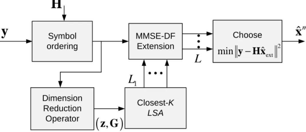
Figure 3.2: Block diagram of the RD-MLS detector.

simple reduction of the search dimension might cause signiﬁcant performance loss, so that a careful mechanism for mitigating such performance loss is needed. In the following section, we propose a dimension reduction algorithm that attempts to mitigate such performance loss, while enabling substantial complexity reduction.

3.3

Reduced Dimension ML Search (RD-MLS)

Algorithm

The structure of the RD-MLS system is depicted in Figure 3.2. The di-mension reduction operator reduces the system didi-mension by suppressing interference, that is, the contribution of symbols not participating in the LTS operation. New observation z and system matrix G obtained from the dimension reduction operator are delivered to the K-LSA block, which per-forms the closest lattice point search over the reduced search space. Since the closest point of the reduced-dimension system is not necessarily equal to the ML solution of the original system, we ﬁnd multiple candidates via LTS. Then, each candidate of the list (denoted as L1) found by theK-LSA is

extended to the full symbol dimension via MMSE-decision feedback (MMSE-DF) estimation. Among the extended list L, a ﬁnal estimate is chosen based on L2-norm criterion.

(26)

3.3.1

Dimension Reduced ML Problem

As the ﬁrst step for dimension reduction, the symbol vectorxis divided into two vectors x1 ∈ Fn1 and x2 ∈ Fn2 (n2 =nt−n1). With knowledge of the

received data yand channel H, the ML solution becomes xml = arg min x∈Fnt∥y−Hx∥ 2 = arg min x1∈Fn1,x2∈Fn2 ∥y−H2x2−H1x1∥ 2 , (3.15)

where H1 and H2 are the sub-matrices constructed by n1 and n2 columns of

H, respectively. Denoting xT ml = [xT1,ml xT2,ml]T, x1,ml can be expressed as x1,ml = arg min x1∈Fn1 ∥y−H2g(y,x1)−H1x1∥2 (3.16) g(y,x1) = arg min x2∈Fn2 ∥y−H2x2−H1x1∥2. (3.17)

Insertion of (3.17) into (3.16) will return to (3.15) and no dimension reduction is therefore achieved. In order to restrict the search space within that spanned byx1, we use a linear estimate ofx2 instead ofg(y,x1). Employing a linear

minimum mean square (MMSE) estimate of x2, i.e., xˆ2, for a given x1, we

obtain the approximate ML estimate, ˜ x1,ml = arg min x1∈Fn1 ∥y−H2xˆ2−H1x1∥ 2 . (3.18)

Assuming that x1 is given, the linear LMMSE estimate ofx2 is

ˆ x2 =f(y,x1) = Rx2y|x1R −1 yy|x1(y−E[y|x1]) (3.19) =HH₂ (H2HH2 +σ 2 wI )₋1 (y−H1x1). (3.20)

Using (3.18) and (3.20), the approximate ML estimate ˜x1,ml becomes

˜ x1,ml = arg min x1∈Fn1 y−H2HH2 ( H2HH2 +σ 2 wI )−1 (y−H1x1)−H1x1 2 . (3.21) Deﬁning the projection operator

Z =σ_w2 (H2HH2 +σ 2

wI

)₋1

(27)

then, (3.21) is written as ˜

x1,ml = arg min

x1∈Fn1

∥Zy−ZH1x1∥2. (3.23)

Further, by denoting z = Zy and G = ZH1, we obtain the integer least

squares problem ˜

x1,ml = arg min

x1∈Fn1

∥z−Gx1∥2. (3.24)

3.3.2

MMSE Dimension Reduction Operator

The preprocessing operation consists of (1) an application of the linear op-erator Z and (2) a tree search over the transformed system. From the rela-tionship y=H1x1+H2x2+w, we can express zas

z=Zy=Gx1+Zr, (3.25)

where r= (H2x2+w). As discussed, H2x2 is an interference term to detect

x1 and the contribution of this term is minimized by the preprocessing. In

fact, from the deﬁnition of Z, one can show that (3.22) can be written as Z= arg min Z′ E [ ∥w−Z′r∥2 ] =RwrR−rr1, (3.26)

which is the LMMSE estimate of w, i.e., ˆw=Zr. Hence, (3.25) becomes

z=Gx1+ ˆw, (3.27)

where ˆw = w+e and e is the LMMSE estimation error. In Section 3.4.1, we will show that the performance of the RD-MLS detector is limited by the detection performance of x1. A potentially useful choice for H1 and H2

would be that which maximizes the receiver SNR for detecting x1 in (3.27),

i.e.,

(H1,H2) = arg max

H′1,H′2SNR(H

′

(28)

where SNR (H′₁,H′₂), E(||Gx1|| 2₎ E(||wˆ||2₎ (3.29) = tr ( ZH′₁(H′₁)HZH) tr ( σ4 w ( H′₂(H′₂)H +σ2 wI )₋1). (3.30)

To obtain an optimal partition from (3.28), (nt

n1

)

= nt!

n1!(nt−n1)! choices would

need to be examined, which is clearly burdensome for a large nt. Thus, a simple scheme such as V-BLAST symbol ordering [11] or probabilistic symbol ordering [23] can be an alternative, where the symbols associated with H1

are detected ﬁrst.

3.3.3

Closest-

K

List Stack Algorithm (

K

-LSA)

As mentioned, due to the reduced dimensionality of the search, ex1,ml is not

guaranteed to be the true ML solution x1,ml, and thus performance loss is

unavoidable. In order to mitigate the loss, a list tree search generating mul-tiple candidates for x1 is employed. In [13], the list SD (LSD) algorithm to

findN best lattice points was proposed. Contrary to the SD algorithm where the radius of the sphere is updated dynamically for each candidate found, the LSD algorithm maintains a fixed radius until it finds the N best points. The radius is updated only when the list is full and a new candidate replac-ing an existreplac-ing one is found. In many cases, therefore, excessive numbers of lattice points are visited, which can easily reduce the benefits of dimension reduction. To maintain the complexity gains of the reduced dimension search while pursuing the performance gain of the LTS, we employ a closest-K list stack algorithm.

As a best-ﬁrst tree search technique, the stack algorithm (SA) [24, 43] extends the node in a tree with the minimum cost metric. For every node extension, node information is stored in the stack and the best node is chosen based on a cost metric of the nodes in the stack. In the reduced system (3.24) described in Section 3.3.1, the cost metric for a tree node Xn′1

(29)

the conversion to the real domain is deﬁned by [30] ai ( Xn′1 i ) = min xi−1∈Ci di−1 ( Xn′1 i−1 ) +ηi−1, (3.31) where di−1 ( Xn′1 i−1 )

is the path metric of the node Xn′1

i−1 (deﬁned in Section

3.2.1), Ci is the set of child nodes of X n′1

i not generated, and ηi is a bias term penalizing short paths [12, 30, 43]. Notice that n′₁ = 2n1 due to the

real conversion. While the search of the SA is finished once it arrives at the first leaf node corresponding to the ML point, the K-LSA continues the search until it finds K −1 additional closest points. However, due to the multiple-lattice-point search, large numbers of back-tracking operations occur. In order to alleviate the complexity increase, theK-LSA employs two measures, a stopping criterion and probabilistic bias, which will be described as follows.

The number of points collected in the candidate list directly impacts the complexity of the RD-MLS detector. In order to adjust the candidate list size effectively, we terminate the search before filling the list via a stopping criterion. After finding the first closest point, the stopping criterion checks if the path metric of the subsequently found closest points d1

(

Xn′1 1

)

satisﬁes the condition, i.e.,d1

(

Xn′1 1

)

> D. Then, the search is stopped if the stopping condition is satisﬁed. In order to choose D, we consider the path metric of the actual transmitted symbols denoted as x1, i.e.,

d1 ( Xn′1 1 ) =∥z−Gx1∥2 =∥wˆ∥2, (3.32)

where ˆw was deﬁned in Section 3.3.2. The parameterD can be chosen such that the probability of the path metric for the transmitted symbols being less than D equals some probability Pϵ, i.e.,

P r(∥wˆ∥2 < D)=Pϵ. (3.33) Since it is hard to ﬁnd D analytically for non-Gaussian ˆw, we introduce a heuristic for choosing D. Using the path metric of ﬁrst found closest point

ˆ Xn′1 1 , we let D=mD1 ( ˆ Xn′1 1 )

, wherem(>1) is called a stopping parameter. Using this condition, the K-LSA collects the points whose path metric is less than m times of that ﬁrst found. The rationale behind this choice is

(30)

that for the case of benign channel/noise conditions (e.g., small ∥wˆ∥2), the path metric of the transmitted symbolx1 is signiﬁcantly smaller than that of

other lattice points, so that it is highly possible to ﬁnd x1 with only a small

number of candidates. In the opposite conditions, many paths have a similar path metric so that the number of candidates should increase in eﬀorts to keep the true solution in the list. Refer to the illustration in Figure 3.3. Due to the stopping criterion, the candidate list size is adjusted to the channel and noise condition and lattice points with dominant metric are stored in the list. In Section 3.4.1, we will show that with this stopping criterion, the LTS oﬀers performance improvement over detection without LTS.

Next, we introduce a method to choose the bias term ηi in (3.31). To compensate the path metric of short paths such that the most likely path chosen to extend appropriately accounts for the diﬀering path lengths of the nodes visited, a proportionate bias term has been used in the tradi-tional stack algorithm [30, 43]. While the bias term ηi in these approaches can be approximate, ηi in our method is chosen by taking into account the contributions of random noise w in the unvisited paths. Speciﬁcally, we model ηi to represent the noise contributions from the unvisited levels of the tree, |w1|2 +· · ·+|wi−1|2, and then assign the probabilistic condition P r(|w1|2+· · ·+|wi−1|2 < ηi

)

=Pprun, where Pprun is the pruning

probabil-ity. For a speciﬁc Pprun, ηi is given by

ηi =Fχ−1(Pprun;i−1). (3.34)

In general, ηi decreases with the tree depth n′1 −i assessing larger bias to

short paths. By using an appropriate value for Pprun (such as Pprun ∼ 0.2

through empirical simulations), we can achieve substantial reduction in back-tracking operations with negligible performance loss. A similar approach has been applied to the SD algorithm in [29] and to SA in [44]. Our approach diﬀers from that of [44] in that rather than using the expected noise power to obtain a bias term, we employ a probabilistic condition (3.34) to choose ηi. Hence, our bias term can be controlled more ﬂexibly through the parameter

(31)

A B C O D 1

Gx

1 ˆ A = + A z Gx w (a) 1

Gx

A B C 1 ˆ B = + B z Gx w O D (b)

Figure 3.3: Illustration of the stopping criterion for the 2×xsystem G. The dark circle O corresponds to the transmitted symbol vector Hx1. The

open circles are the observed signal vectors for two scenarios of (a) bad and (b) good noise conditions, i.e., ∥wˆA∥2 >∥wˆB∥2. As shown in the ﬁgure, for bad noise realizations, the points near the observed vector zA are likely to have a similar distance metric so that many lattice points are collected. On the other hand, for good noise realizations, only a few lattice points have small distance metric. With high probability, the ML point will be found among them. The stopping criterion with m = 1.5 selects the points inside the gray circle as candidates, and hence it collects {A, B, C, O}for the case (a) and only {O} for the case (b).

(32)

3.3.4

Postprocessing

The postprocessing operates in two steps. First, for each of the candidates forx1 obtained by the LTS, we generate the symbol vectors of full dimension

by concatenating them with the MMSE-DF estimates of x2. Then, among

those vectors, we choose one minimizing the Euclidean distance metric as the ﬁnal output.

We assume that the columns ofH2 and entries ofx2are arranged based on

the detection ordering provided in [23] or [11]. We let ˆxi

1 be the ith element

in the candidate list and ˆxi

2 = [ˆxi2,1,· · ·,xˆi2,n2]

T _{be the corresponding} MMSE-DF estimate of x2 given ˆxi1. Further, we let h2,k be the kth column of H2.

To obtain the MMSE-DF estimate of x2, for each candidate of L, we ﬁrst

subtract the eﬀect of ˆxi

1 from y, i.e., yi = y−H1ˆxi1, and then obtain the

estimates ˆxi₂_,₁,· · · ,xˆi₂_,n₂ successively. The MMSE-DF detection steps can be summarized as follows:

STEP 1 : Compute yi =y−H1xˆi1 for all i= 1,· · · , K.

STEP 2 : (Iteration) for all i= 1,· · · , K, for k = 1 :n2, compute ˇ xi₂_,k =f_kHy(_ik) (3.35) ˆ xi₂_,k =slicer(xˇi₂_,k) (3.36) y_i(k+1) =y(_ik)−h2,kxˆi2,k (3.37) end

Here “slicer” denotes the function of mapping the complex-valued ˇxi₂ to the nearest transmitted constellation point. The MMSE-DF ﬁlter coeﬃcient fk is given by [45, 46] fk = ( _n 2 ∑ j=k h2,jhH2,j+σ 2 wI )−1 h2,k. (3.38) Once ˆxi

(33)

ﬁnal list search as L={xˆ1_ext,· · · ,xˆK_ext} = {[ ˆ x1 1 ˆ x1 2 ] ,· · · , [ ˆ xK 1 ˆ xK 2 ]} (3.39) and the element of L minimizing the cost function (3.40) becomes the ﬁnal output of the RD-MLS e xml = arg min a∈L ∥y−Ha∥ 2 . (3.40)

The whole detection procedure of the RD-MLS algorithm is summarized in Appendix A.

3.4

Discussion

The two key parameters aﬀecting the complexity and performance of the RD-MLS are the dimension n1 and stopping parameter m. In this section,

we present the performance analysis for the RD-MLS and show how these parameters aﬀect error performance.

3.4.1

Performance Analysis

The aim of this subsection is to derive an upper bound on the detection error probability for the RD-MLS. To make the analysis tractable, we consider the case where the system matrix His partitioned without any column ordering so that the elements of H1 andH2 are assumed to be random i.i.d. complex

Gaussian. That is, we disregard the partitioning criterion described in Sec-tion 3.3.2 for the simplicity of analysis. The detecSec-tion error probability of the RD-MLS detector, Perr, is deﬁned as

Perr=

∑

xA

Pcer(xA)P(xA), (3.41)

whereP (xA) is thea priori probability thatxAwas transmitted andPcer(xA) is the conditional error rate (CER) that xA is not detected by the RD-MLS given that xA was transmitted. Recalling that the ﬁnal output chosen from

(34)

the list L is denoted as exml_, _P

cer(xA) becomes

Pcer(xA) =P rA(exml ̸=xA) (3.42)

=P rA ( e xml ̸=xAxA ∈ L ) P rA(xA∈ L) +P rA ( e xml ̸=xAxA∈ L/ ) P rA(xA∈ L/ ), (3.43) where P rA(B) refers to the conditional probability of event B under the condition that xA was transmitted. Let xml be an exact ML solution. We

denote PML

e (xA) =P rA(xml ̸=xA), which is the ML detection error proba-bility given xA was sent. Then, we have

P rA ( e xml ̸=xAxA ∈ L ) ≤P rA ( xml ̸=xAxA∈ L ) (3.44) ≤ P rA(xml ̸=xA,xA∈ L) +P rA(xml ̸=xA,xA ∈ L/ ) P r(xA∈ L) (3.45) = P ML e (xA) P r(xA∈ L) , (3.46)

where (3.44) follows from the fact that the RD-MLS chooses a closest point from L while the ML detector does from all candidate points. From (3.46) and the fact that P rA

( e xml_̸₌_x AxA∈ L/ ) = 1, (3.43) becomes Pcer(xA)≤PeML(xA) +P rA(xA ∈ L/ ). (3.47) The second term in the right-hand side of (3.47) illustrates the primary source of sub-optimality of the RD-MLS. Following symbol partitioning, let xA be divided into xA1 and xA2. Let the corresponding partitioned candidate sets

be L1 = { ˆ x1 1,· · · ,xˆK1 } and L2 = { ˆ x1 2,· · · ,xˆK2 }

. We can show that (3.47) becomes

Pcer(xA)≤PeML(xA) +P rA(xA∈ L|/ xA1 ∈ L/ 1)P rA(xA1 ∈ L/ 1)

+P rA(xA∈ L|/ xA1 ∈ L1)P rA(xA1 ∈ L1) (3.48)

≤P_eML(xA) +P rA(xA1 ∈ L/ 1) +P rA(xA2 ∈ L/ 2|xA1 ∈ L1).

(35)

where (3.49) follows fromP rA(xA ∈ L|/ xA1 ∈ L1) =P rA(xA2 ∈ L/ 2|xA1 ∈ L1)

and P rA(xA ∈ L|/ xA1 ∈ L/ 1) = 1. The second and third terms on the

right-hand side in (3.49) are the probability that the candidate list found by the LTS does not containxA1 and the conditional probability that the MMSE-DF

estimation makes a decision error given the LTS yielded xA1 in L1,

respec-tively. We denote these terms as PLTS

e and PeMMSE−DF, respectively. From (3.41) and (3.49), an upper bound of Perr is written

Perr≤PeML+ ∑ xA1 ∑ xA2 P rA1,A2(xA1 ∈ L/ 1)P (xA1,xA2) +∑ xA P rA(xA2 ∈ L/ 2|xA1 ∈ L1)P (xA) (3.50) =P_eML+∑ xA1 P rA1(xA1 ∈ L/ 1)P (xA1) | {z } PLTS e +∑ xA P rA(xA2 ∈ L/ 2|xA1 ∈ L1)P (xA) | {z } PeMMSE−DF , (3.51)

whereP rA1(·),P(xA1), andP (xA1,xA2) are deﬁned similarly asP rA(·) and

P (xA).

To investigate the asymptotic behavior of P_eLTS, we consider the input to the LTS in (3.27), z = GxA1 + ˆw. We remind the reader that G = ZH1,

ˆ

w=w+e and e =Z(H2x2+w)−w. Using these, we can write z by

z=GxA1+ZH| 2x{z2+Zw} ˆ

w

. (3.52)

Thoughx2 is discrete inFn2, we approximate the LMMSE estimation error

plus noise, ˆw(= w+e) as a complex Gaussian vector with zero mean and the covariance matrix Φ=E[( ˆw)( ˆw)H] =σ_w4 (H2HH2 +σ2wI

)−1

. For large SNR, we note that ZH2 becomes zero matrix while Z does not vanish as σ2w →0 (see Appendix B). From (3.52) and also using this result, ˆw approximates to a Gaussian distribution as SNR increases. Asymptotic normality of this type of interference plus noise term for MMSE detection was also validated in [47] and [48].

(36)

approx-imation, we show in Appendix C that P rA1(xA1 ∈ L/ 1) is upper-bounded by P rA1(xA1 ∈ L/ 1)≤cEH2 [_n r ∏ i=1 λ1 λ2 i λ1 λ2 i +_λm2 ] , (3.53)

where λ is the normalization factor of the QAM modulation,λ1 ≥ · · · ≥λnr

are the eigenvalues of (H2HH2 +σw2I

)−1

, and c = Mn1 −_{1. The notation}

EH2[·] implies an expectation taken over H2. We consider the high SNR

regime of (3.53) as σ2_w → 0. If we let P(≤ n2) be the rank of H2, it follows

that λ1 = · · · =λnr−P = 1/σ 2

w and λi = 1/(qnr−i+1+σ 2

w) for nr−P + 1 ≤

i ≤nr, where q1,· · · , qP are the (non-zero) eigenvalues of H2HH2 . Then, we

have P rA1(xA1 ∈ L/ 1)≤cEH2 [_n r−P ∏ i=1 λ1 λ2 i λ1 λ2 i + m λ2 nr ∏ i=nr−P+1 λ1 λ2 i λ1 λ2 i + m λ2 ] (3.54) ≤cEH2 [_n r−P ∏ i=1 λ1 λ2 i λ1 λ2 i + m λ2 ] (3.55) ≤c nr∏−n2 i=1 ( σ2_w σ2 w + m λ2 ) (3.56) =c ( 1 1 + m λ2_σ2 w )nr−n2 (3.57) ≤c ( λ2_σ2 w m )nr−n2 , (3.58)

where the inequality in (3.55) gets tighter asσ2_w →0 since λ1

λ2

nr−P+1

,· · ·, λ1

λ2

nr →

∞and (3.56) holds becauseλ1 =· · ·=λnr−n2 = 1

σ2

w regardless of realizations

of H2. Since this upper bound does not depend onxA1, it becomes an upper

bound of PLTS

e .

From (3.58), we can provide some important observations on the asymp-totic behavior of the RD-MLS. First, we observe that the upper bound is a decreasing function of the list stopping parameter m. This follows our intu-ition as, whenmincreases, the number of candidates in the list also increases, and the eﬀect of additional loss decreases. Since m multiplies the ratio of the minimum squared distance 4/λ2 _{to the noise power} _σ2

w, it provides ad-ditional eﬀective SNR gains over the single candidate search. Second, we observe that the diversity gain (= limSN R→∞−log_logBER_{SN R}) of the term related

(37)

Table 3.1: Complexity of RD-MLS algorithm.

Block # of real additions # of real multiplications Dimension reduction step (Preprocessing) 4n2

r−2nr 4n2r

Postprocessing step K(8nt−4n1−4)nr−K(2nt−2n1) K(8nt−4n1−4)nr

Nkfor theK-LSA 2nt−k+ 7 2nt−k+ 5

to P_eLTS is larger than or equal to nr−n2(=nr−nt+n1).

We next take a look at the probabilityP_eMMSE−DF. This is the probability that the MMSE-DF estimation makes a decision error for the systemH2x2+

w resulting from perfect cancellation of xA1 in (3.35). It is well known

that the MMSE-DF detector for the nr-by-n2 system achieves a diversity

of nr −n2 + 1 both with and without the ordering based on post-detection

SNR [11, 49].

Based on (3.51), at high SNR, the diversity gain would be dominated by

nr+n1−nt, which is the minimum of those for PeML, PeLTS, andPeMMSE−DF, i.e., min (nr, nr+n1−nt , nr+n1 −nt+ 1). In fact, this diversity gain is the same as that achieved by the scheme employing a single candidate search [35]. However, owing to the p