Repositorio Institucional de la Universidad Autónoma de Madrid
https://repositorio.uam.es
Esta es la versión de autor del artículo publicado en:
This is an author produced version of a paper published in:
Neurocomputing 74.12-13 (2011): 2250 – 2264
DOI: http://dx.doi.org/10.1016/j.neucom.2011.03.001
Copyright: © 2011 Elsevier
El acceso a la versión del editor puede requerir la suscripción del recurso Access to the published version may require subscription
Empirical Analysis and Evaluation of Approximate
Techniques for Pruning Regression Bagging Ensembles
Daniel Hern´andez-Lobato∗,a, Gonzalo Mart´ınez-Mu˜nozb, Alberto Su´arezb
a
Machine Learning Group, ICTEAM Institute, Universit´e catholique de Louvain, Place Sainte Barbe 2, B-1348 Louvain-la-Neuve, Belgium.
b
Computer Science Department, Escuela Polit´ecnica Superior,
Universidad Aut´onoma de Madrid,
C/ Francisco Tom´as y Valiente, 11, Madrid 28049 Spain.
Abstract
Identifying the optimal subset of regressors in a regression bagging ensemble is a difficult task that has exponential cost in the size of the ensemble. In this article we analyze two approximate techniques especially devised to address this problem. The first strategy constructs a relaxed version of the problem that can be solved using Semidefinite Programming. The second one is based on modifying the order of aggregation of the regressors. Ordered Aggregation is a simple forward selection algorithm that incorporates at each step the re-gressor that reduces the training error of the current subensemble the most. Both techniques can be used to identify subensembles that are close to the optimal ones, which can be obtained by exhaustive search at a larger com-putational cost. Experiments in a wide variety of synthetic and real-world regression problems show that pruned ensembles composed of only 20% of the initial regressors often have better generalization performance than the orig-inal bagging ensembles. These improvements are due to a reduction in the bias and the covariance components of the generalization error. Subensem-bles obtained using either SDP or Ordered Aggregation generally outperform subensembles obtained by other ensemble pruning methods and ensembles generated by the Adaboost.R2 algorithm, negative correlation learning or regularized linear stacked generalization. Ordered Aggregation has a slightly
∗Corresponding author. Tel: +32-10-47-2445; fax: +32-10-45-0345.
Email addresses: [email protected](Daniel
Hern´andez-Lobato),[email protected] (Gonzalo Mart´ınez-Mu˜noz),
better overall performance than SDP in the problems investigated. How-ever, the difference is not statistically significant. Ordered Aggregation has the further advantage that it produces a nested sequence of near-optimal subensembles of increasing size with no additional computational cost.
Key words: Regression, Ensemble Learning, Bagging, Boosting, Semidefinite Programming, Ensemble Pruning
1. Introduction
Ensembles have the potential to improve the performance of an individ-ual predictor by combining the outputs of a collection of complementary predictors. A widely used algorithm to build ensembles for classification and regression is bagging [6]. In bagging, different models are generated by ap-plying the same learning algorithm to independent bootstrap samples of the original training data. If the learning algorithm used is unstable (that is, if small changes in the training set lead to different models), a collection of diverse regressors can be induced from the different bootstrap samples. If the errors of these elements are uncorrelated, improved predictions can be obtained by averaging the outputs of the regressors in the ensemble. This mechanism generally reduces the variance component of the generalization error [7, 8, 49]. Bagging is a very robust learning algorithm, which can per-form well even when data are noisy [17, 41]. Furthermore, including more elements in a bagging ensemble does not generally lead to overfitting [11]. Typically, the prediction error decreases monotonically with the ensemble size, and asymptotically approaches a constant level, which is considered the best result that bagging can achieve.
Another popular ensemble algorithm is boosting. Boosting was originally developed for classification problems [19, 46]. In boosting, a sequence of models is induced from a given dataset using a fixed learning algorithm and different weights for the different training instances. The first model in the sequence is learned using equal weights. The (n+ 1)th model in the ensemble is constructed by modifying the weights of the instances used for induction: Larger weights are assigned to training examples that are incorrectly labeled by the nth model in the sequence. By contrast, the weights of correctly labeled instances are lowered. The final prediction of the boosting ensemble is a weighted combination of the predictions of the individual models. The weights in this combination are determined by the error on the training
data: The lower the training error of the model, the higher its weight in the ensemble prediction and vice versa. Boosting has been shown to perform well in several benchmark classification problems [3, 9, 41]. However, it is very sensitive to noise in the class labels and its effectiveness is severely reduced in noisy domains [17, 41]. Boosting has also been adapted to solve regression problems [1, 18, 19, 21]. In this work we use the Adaboost.R2 algorithm, one of the extensions of Adaboost for regression proposed in [18]. This variant of boosting has been selected because of its good performance in several regression problems [18]. Furthermore, Adaboost.R2 is used as a benchmark for comparison in previous work on regression ensembles [12, 56, 1].
An important shortcoming of ensemble methods is that, in many prob-lems of practical interest, many predictors are needed to achieve good gener-alization performance. Large ensembles require more storage space and take longer to make predictions. A possible way to alleviate this problem is to replace the original ensemble by a representative subset of predictors. This approach has been shown to be effective in classification problems: Pruned subensembles can in fact outperform the original ensembles from which they are extracted [2, 13, 30, 33, 34, 35, 55, 31]. Nevertheless, the task of se-lecting from a pool of predictors a subset whose performance is optimal is a difficult problem. On the one hand, it is computationally expensive: The search is conducted in the space of 2M−1 non-empty subensembles that can be extracted from an ensemble of size M. On the other hand, even if the search were feasible, the selection is made in terms of an objective function estimated on the training data. Since we are interested in out-of-sample per-formance, finding the optimum in the training set does not guarantee optimal generalization properties.
Previous studies have shown that the generalization performance of re-gression bagging ensembles can be improved by selecting a subset of com-plementary regressors whose prediction errors are uncorrelated [39, 56, 26]. These techniques can be used in principle to prune other types of ensembles in which the final prediction is obtained by averaging over the individual predictors that make up the ensemble [44, 54, 37, 32]. The main goals of this research are to design extensions to regression problems of pruning tech-niques that have been previously introduced in the context of classification problems, to analyze their properties and to evaluate their performance. The first technique investigated is an adaptation of the pruning method based on Semi-definite Programming (SDP) introduced in [55]. An alternative ap-proach to ensemble pruning consists in modifying the order of aggregation in
the ensemble [31]. Starting with an empty subensemble, Ordered Aggrega-tion follows a forward selecAggrega-tion strategy and incorporates the regressor that reduces the training error of the current subensemble the most, until a stop-ping criterion is met. In the current work we show that the subensembles identified by the ordering procedure are very similar both in performance (quantified in terms of either the training error or the test error) and in com-position to optimal subensembles of the same size, identified by exhaustive search. The optimality of the subensembles is determined in terms of the training set alone, which are the only data available for induction.
As noted earlier, minimizing a measure of performance on the training set does not necessarily lead to improvements in generalization capacity. To evaluate the generalization performance of the pruned subensembles and to compare it with other ensemble generation and ensemble-pruning methods, we carry out extensive experiments in 24 synthetic and real-world datasets. The results of these experiments show that SDP-pruning and Ordered Aggre-gation are effective methods for identifying subensembles with good general-ization performance not only in classification problems, but also in regression tasks. A detailed analysis of the components of the generalization error of the subensembles confirms that the improvements in prediction accuracy arise because both SDP-pruning and Ordered Aggregation select from the original ensembles subsets of regressors that simultaneously have a low bias (i.e. their individual errors tend to be low) and small or negative correlations (i.e. their predictions are complementary).
In the problems investigated, and for a large range of pruning rates, pruned subensembles obtained with these two methods outperform single neural networks, complete ensembles built either with bagging or Adaboost.R2 and other pruning techniques based on genetic algorithms [56]. The differ-ences observed are statistically significant. The performance of the subensem-bles identified via SDP-pruning or by Ordered Aggregation is comparable with the subensembles identified by other pruning methods described in the literature [39] and with the ensembles generated by negative correlation learn-ing [29] or regularized linear stacked generalization [43]. The overall perfor-mance of Ordered Aggregation is slightly better than SDP. However, the difference is too small to be statistically significant. The simple forward se-lection used in Ordered Aggregation has the advantage of producing a nested sequence of near-optimal subensembles of increasing size. By contrast, SDP requires to solve a different semi-definite programming problem for each en-semble size, which entails a correlative increase in computational costs.
The article is organized as follows: Section 2 introduces the problem of selecting an optimal subensemble from a pool of regressors generated with bagging. Since this problem is NP-hard, approximate methods have to be used in practice. Near-optimal solutions can be found by SDP-pruning or by Ordered Aggregation. An empirical analysis of these techniques is pre-sented in Section 3. Specifically, Section 3.1 shows that the subensembles identified using either SDP-pruning or Ordered Aggregation are very close to the optimal subensembles obtained by exhaustive search. These near-optimal subensembles actually outperform the original complete ensembles from which they are extracted. The bias-variance-covariance analysis pre-sented in Section 3.2 elucidates the origin of the improvements obtained. The results of the extensive assessment of the performance of the pruning methods analyzed are presented in Section 3.3. Finally, Section 4 summarizes the results and conclusions of this work.
2. Selection of Optimal Subensembles
Consider a regression problem. The goal is to learn a function that pre-dicts the dependent variable y ∈ R in terms of the attributes x ∈ X using a set of training data D = {(x1, y1), ...,(xN, yN)}, whose instances are in-dependently drawn from a probability distribution P(x, y). Bagging works by combining the prediction of a collection of regressors. Each of these re-gressors is constructed by applying a fixed learning algorithm on a different bootstrap sample from the original training data D. Let ˆfi(x) be the pre-diction given by the ith regressor built with Di, the ith bootstrap sample from the training data. The prediction of the ensemble is the average of the individual predictions of the M regressors in the ensemble
M−1 M X i=1 ˆ fi(x), i= 1,2, . . . , M. (1) The generalization error of the ensemble is
L = Z M−1 M X i=1 ˆ fi(x)−y !2 P(x, y)dxdy, (2) where y =f(x), f is the target function to approximate, and P(x, y) is the probability distribution of the data. After some algebra (2) can be expressed
as L =M−2 M X i=1 M X j=1 Cij (3) where Cij = Z ˆ fi(x)−y fjˆ(x)−yP(x, y)dxdy . (4) The value Cii is the average squared error of the ith ensemble member. The off-diagonal terms {Cij, i6=j} correspond to correlations between the pre-dictions of the ith and jth ensemble members [56, 39].
Consider a bagging ensemble of sizeM. Our goal is to select the subensem-ble of uregressors {s1, s2, . . . , su} that minimizes the error
L(u)=u−2 u X i=1 u X j=1 Csisj, (5)
where{s1, s2, . . . , su}is a subset of the indices that label the ensemble
mem-bers{1,2, . . . , M}. Since the actual generalization error cannot be computed, the selection of the optimal subensemble is made on the basis of the training error. The expression for the training error is identical to (5), except that the average over P(x, y) in the calculation of Cij is replaced by a sample average over the training data
Cij(tr) = 1 N N X n=1 ˆ fi(xn)−yn fj(ˆ xn)−yn). (6) Hence, the information needed for the optimization problem is contained in the matrix C(tr), which is estimated on the training set. This estimate is
expected to be close to the true C matrix, which is calculated as an
aver-age over the actual distribution of the data, so that minimizing the train-ing error leads to the minimization of the generalization error. This is not necessarily the case in actual regression problems: minimizing the training error sometimes leads to overfitting, and, consequently, to the selection of subensembles whose generalization performance is suboptimal. In the exper-iments performed, overfitting becomes manifest in the fact that, typically, the subensembles that minimize the error on the training data tend to be smaller than the subensembles that are optimal when the error is estimated on an independent test set.
In any case, even if it were possible to accurately predict the generaliza-tion error from the training data only, finding the optimal subensemble is a computationally expensive problem that involves comparing the performance of all the possible 2M−1 non-empty subensembles that can be extracted from the original ensemble. In fact, the problem of selecting the optimal subensem-ble from a given ensemsubensem-ble is NP-hard (see Appendix A). This implies that finding the exact solution is infeasible for large ensembles. In this work we analyze two techniques that can identify near-optimal subensembles at a re-duced computational cost1. The first method solves a relaxed version of the
problem using semidefinite programming (SDP). The second one is based on modifying the order of aggregation of the regressors in the ensemble, which in standard bagging is random.
2.1. Ensemble pruning via semidefinite programming
The method based on Semidefinite programming (SDP) introduced in [55] by Zhang et al. to prune classification ensembles can be extended to ensembles of regressors. In classification tasks the subensemble selection problem is formulated in terms of an M × M matrix G, whose diagonal terms Gii measure the individual training errors of the ensemble members and whose off-diagonal terms Gij, i 6= j measure the number of common training errors between classifiersi andj. The goal is to find the sub-matrix of G, of dimensions u×u, that corresponds to a subensemble of size u that minimizes the sum of the elements in G. This process need not provide the subensemble of size u with the minimum training error. However, it guarantees that the subensemble elements have small training error rates and that they tend to make incorrect predictions for different training instances. The problem described in the previous paragraph is a standard 0-1 opti-mization problem that is also NP-hard. Zhanget al. reformulate this problem so that it has the same optimal solutions as an instance of the max-cut prob-lem of size u (MC-u). This problem consists in partitioning the vertices of an edge-weighted graph into two sets, one of which has as sizeu, so that the total weight of edges crossing the partition is maximized. Good approximate solutions to the max-cut problem can be obtained using an algorithm based on SDP [23, 24]. Therefore, good approximations to the problem of selecting
1Source code available for both pruning techniques at
an optimal subensemble of size ucan be found by solving the corresponding instance of the MC-u problem.
The ensemble pruning problem of Zhang et al. is formulated in [55] as min u u TGu s.t. P iui =u, ui ∈ {0,1}, (7)
The binary variableui takes the value 1 ifith predictor is selected and 0 if it is not selected. Without the cardinality constraint,P
iui =u, there is a trivial solution to the problem, in which none of the regressors is selected. They then propose the transformationui = (vi+ 1)/2 withvi ∈ {−1,1}. With this change of variables, the objective function is proportional to (v+e)TG(v+e), where e is a column vector composed ofM ones. The constraint P
iui =u becomes (v+e)TI(v+e) = 4u, where I is the identity matrix. Defining the matrices H = eTGe eTG Ge G , D = M eT e I , (8)
and extending the vector v with one additional component v0 that takes
value one, (7) becomes min v v THv s.t. vTDv = 4u, v0 = 1, vi ∈ {−1,1} ∀i6= 0. (9)
This problem is equivalent to min v H•vv T s.t. D•vvT = 4u, v0 = 1, vi ∈ {−1,1} ∀i6= 0. (10) where A•B=P
ijAijBij. This latter formulation of the problem is equiv-alent to the MC-u problem [55]. The goal is now to construct the relaxed version of the problem that can be efficiently solved using SDP. The con-straint v0 = 1 in (10) is relaxed to v0 ∈ {−1,1} without modifying the
problem, because−vis feasible whenevervis feasible. Next, the constraints vi ∈ {−1,1} are rewritten in the form diag(vvT) =e
min v H•vv T s.t. D•vvT = 4u, diag(vvT) =e. (11)
The problem can be expressed in terms of a positive semidefinite matrix V
of rank one min V H•V s.t. D•V= 4u, diag(V) =e, V 0. rank(V) = 1. (12)
This reformulation is possible because vvT = V if and only if V 0 and rank(V) = 1.
From this reformulation it is possible to obtain a convex SDP optimization problem from (12) by dropping the rank constraint
min V H•V s.t. D•V= 4u, diag(V) =e, V 0. (13)
This SDP problem can be efficiently solved in polynomial time with a suit-able optimizer, such as the one designed in [5]. As described in [55], from a solution matrix V of (13), a solution vector u is obtained by a random-ized approximate algorithm [23, 24]. Specifically, the components of u are determined by sampling v from a Gaussian distribution N(0,V) and then applying the rule
ui = (
1 if sign(vi) = sign(v0)
0 if sign(vi)6= sign(v0)
. (14)
If the targeted number of regressors in the subensemble is not correctly de-termined by the application of this rule, Zhanget al. use a greedy algorithm that incorporates or removes elements in u, as needed, causing the least de-terioration in (7). This procedure is repeated ten times and the best solution is retained.
Even though (13) can be cast in a form that is equivalent to the MC-u
problem, the approximation bounds that hold for the relaxed version of this problem [23, 24] are not applicable in the relaxed version of subset selection. Subset selection and the MC-u problem share optimal solutions but not opti-mal values. The reason is that the objective function in (13) does not exactly match the objective in the MC-u problem [55]. Despite this lack of guaran-tees for the quality of the approximation, the procedure described is very effective in selecting near-optimal ensembles in classification tasks [55, 31].
The approach described above for pruning classification ensembles can be extended to prune regression ensembles. For this, we observe that the generalization error of the initial bagging ensemble can be expressed in terms of the matrix C in (3). Thus, the subensemble selection problem consists
in finding a subensemble of size u for which the sum of the elements in the corresponding sub-matrix ofCis as low as possible. An approximate solution
to this problem can be obtained using the method of Zhang et al. to prune classification ensembles. The difference lies in the matrix that is used to guide the optimization process. In [55] it is the matrix G. In the regression case, this matrix is replaced by an appropriate estimate of the matrixC, the
matrixC(tr), defined in (6). The diagonal elements of this matrix measure the
individual squared errors on the training set, and the off-diagonal elements correspond to correlation-like values.
The computational cost of selecting a subensemble of size u by solving problem (13) is O(M3), where M is the size of the initial ensemble. The
computation of C(tr) is O(M2 · N). Therefore, the total cost of the SDP
method for pruning regression ensembles is O(M3 +M2 ·N), where N is
the size of the training set D. Extracting all near-optimal subensembles of sizes u = 1,2, . . . , M, implies solving (13) M times, with an overall cost
O(M4+M3·N).
2.2. Ordered Aggregation
Another strategy that can be used to find an approximate solution to the subensemble selection problem is based on modifying the order in which the predictors are aggregated into the ensemble. This strategy has been suc-cessfully used for pruning classification ensembles [13, 30, 33, 34, 35, 45, 31]. Specifically, one of the goals of [31] was to determine the relevance of the choice of ordering heuristic to the performance of the resulting pruned en-sembles. The conclusion of that study is that the effectiveness of different heuristics that take into account both the individual prediction accuracy and
the complementarity of the classifiers is very similar. The goal of the present work is to extend this analysis to regression problems, where the optimiza-tion of the training error provides a natural criterion for the selecoptimiza-tion of subensembles. The effectiveness of Ordered Aggregation in regression bag-ging ensembles was assessed in [26]. In the present investigation we provide a more detailed analysis of Ordered Aggregation and a more extensive eval-uation, including comparisons with related ensemble creation and ensemble pruning methods, such as negative correlation learning, SDP-pruning, the pruning method proposed by Perrone and Cooper [39], the genetic algorithm described in [56] and regularized linear stacked generalization ensembles ob-tained using the lasso [43].
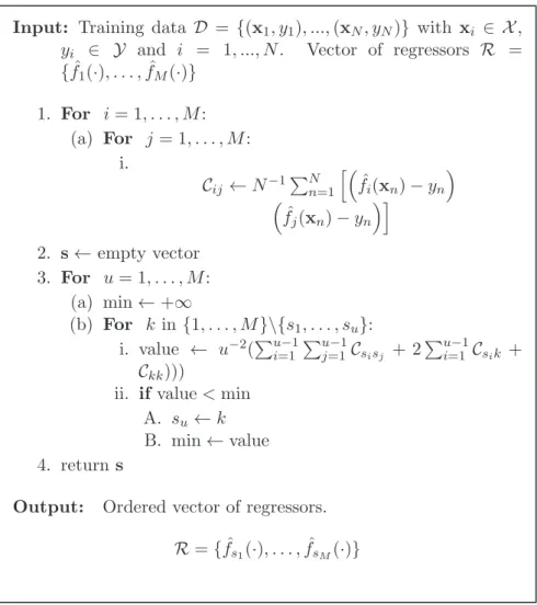
From the initial pool ofM regressors generated by bagging, ordered ag-gregation builds a sequence of nested ensembles, in which the ensemble of size u contains the ensemble of size u− 1. The algorithm starts with an empty ensemble that grows by incorporating at each iteration the regressor that reduces the training error of the enlarged subensemble the most. In par-ticular, the regressor selected in the uth iteration is the one that minimizes the expression su = arg min k u−2( u−1 X i=1 u−1 X j=1 C(tr) sisj + 2 u−1 X i=1 Cs(tr) ik +C (tr) kk ) (15)
where k ∈ {1, .., N}\{s1, s2..., su−1} and {s1, s2..., su−1}label regressors that
have been incorporated in the pruned ensemble at iteration u−1. Fig. 1 displays the pseudo-code for Ordered Aggregation.
This process can be seen as an ordering of the regressors of the complete ensemble because the subensemble generated at iteration u includes all the regressors of the subensemble generated at iteration u−1. The subensemble of size u with 1 ≤ u ≤ M is obtained by taking the first u regressors from the ordered sequence. Subensembles selected by Ordered Aggregation need not be optimal. In particular, the optimal subensemble of size u (the one with the lowest mean squared error on the training data) need not include all the regressors of the optimal ensemble of sizeu−1. Nonetheless, Ordered Aggregation is expected to identify near-optimal solutions of the subensemble selection problem.
The time-complexity of this algorithm, as a function of the number of regressors in the bagging ensemble, can be readily estimated. Each of theM iterations requires the extraction of the regressor that minimizes (15) from
Input: Training data D = {(x1, y1), ...,(xN, yN)} with xi ∈ X,
yi ∈ Y and i = 1, ..., N. Vector of regressors R =
{fˆ1(·), . . . ,fˆM(·)} 1. For i= 1, . . . , M: (a) For j= 1, . . . , M: i. Cij ←N−1PNn=1 h ˆ fi(xn)−yn ˆ fj(xn)−yn i 2. s← empty vector 3. For u= 1, . . . , M: (a) min←+∞ (b) For k in{1, . . . , M}\{s1, . . . , su}: i. value ← u−2(Pui=1−1Puj=1−1Csisj + 2 Pu−1 i=1 Csik + Ckk)))
ii. ifvalue<min A. su ←k
B. min←value 4. return s
Output: Ordered vector of regressors. R={fˆs1(·), . . . ,fˆsM(·)}
the remaining pool of regressors. This task has a cost O(((M + 1)−u)·u), where 1 ≤ u ≤ M is the current iteration. Therefore, the total complexity of the ordering is O(M3). Finally, because computing C(tr) takes O(M2 ·
N) steps the final cost is O(M3 +M2 ·N). In contrast to SDP-pruning,
where selecting subensembles of different sizes requires separate executions of the algorithm, Ordered Aggregation generates a sequence of near-optimal subensembles of increasing size at no additional cost.
2.3. Related work
The key to the improvements in the performance of the ensemble is the complementarity of the predictions given by the individual ensemble members [12, 17, 26, 49]. Individual measures of accuracy or measures of diversity cannot be used in isolation to improve the performance of the ensemble. Successful ensemble pruning techniques need to encourage complementarity among the selected predictors.
The idea of modifying the order in which the classifiers are aggregated in the ensemble was introduced as a possible improvement of ensemble learning in [39] by Perrone and Cooper. However, the order of aggregation proposed in that work is based on the individual properties of the ensemble members (e.g. the mean squared error of each neural network). The joint performance of the predictors is considered only at a later stage, to decide whether a candidate neural network does not lead to a reduction of the subensemble error and should therefore be excluded from the current subensemble. Specifically, [39] suggests to swap such a network with the closest un-tested network in the ordered sequence. The pruning method stops when none of the un-tested networks in the ordered sequence provide a reduction of the subensemble error.
Building an ensemble of regressors whose predictions have small or neg-ative correlations is one of the design goals of negneg-ative correlation learning [29]. In this learning algorithm, diversity is encouraged by simultaneously training a collection of networks using a cost function that includes a cor-relation penalty term in addition to the prediction error. The corcor-relation penalty term encourages the specialization of the individual networks and cooperation among them. However, the strength of the penalty needs to be to be carefully tuned for each problem. If it is too small, the cooperation among the ensemble members will not be sufficient to produce significant im-provements in performance. If the penalty is too large, the learning process is ineffective: the cost function is dominated by the penalty term and becomes
insensitive to prediction errors. A further difficulty of this method is that the correlation penalty introduces a coupling among the parameters of the different ensemble members. This coupling increases the dimensionality of the parameter space in which the search is conducted and makes the learning process more difficult.
Genetic algorithms (GAs) have also been proposed for the selection of a near-optimal subensemble from a complete bagging ensemble. In [56] the output of the ensemble is a weighted average of the outputs of each ensemble member. The optimal set of weights of the ensemble members is found by minimizing a function that estimates the generalization error of the ensemble. The minimization problem is solved by GASEN (Genetic Algorithm based Selective ENsemble), a standard GA with a floating-point encoding scheme for the real-valued weights. Once evolution has finished, the neural networks whose optimized weights are below a specified threshold are removed from the ensemble. The final ensemble output is the average over the predictions of the networks retained in the ensemble. The experiments carried out in [56] establish GA as a viable strategy to prune bagging ensembles. However, the ensembles considered in that work are rather small. In fact, for the ensemble sizes considered (20 networks) exhaustive search is still feasible. In this work we show that this GA can also be used to extract subensembles with good prediction properties from larger ensembles, such as the ones typically generated in bagging (≈100 learners).
Subset selection techniques [25, 36] can also be used to identify subsets of predictors that outperform the original complete ensemble. The stacked generalization method described in [43] is illustrative of this approach. In stacked generalization, the vector of predictions of the different ensemble members for each training sample is considered as a data instance in a new feature space [53]. These instances are then used to train a meta-learner that produces the final ensemble prediction. In practice, the predictor used for output combination can be built using any learning algorithm. There is extensive empirical evidence that stacking predictors tends to overfit unless the combiner function is sufficiently smooth [43]. Specifically, linear combi-nations generally perform better than non-linear models [48]. Nevertheless, when the number of the predictors in the ensemble is large, even linear mod-els tend to overfit [13]. This problem can be alleviated by the application of regularization techniques [43]. If regularization is performed via the lasso [47] or the elastic net regression [57] some of the coefficients of the linear model will take value zero. Therefore, the corresponding predictors can be removed
from the ensemble, because they are not involved in the combined prediction. In contrast to the ensemble pruning methods considered in this work, which assume equal weights, the remaining predictors can have different weights in the final prediction. In this work, we analyze the performance of ensem-bles of this type generated via stacking combined with lasso regularization. Instead of the lasso other subset selection techniques can be used [36]. Ex-periments on a variety of regression problems show that variants of these subset selection techniques in which uniform weights are used (instead of the actual non-zero weights calculated) have poorer generalization performance. In consequence, these variants are not considered for further evaluation.
3. Empirical Analysis and Evaluation
In this section we carry out an empirical analysis of SDP-pruning and Ordered Aggregation and evaluate their performance. For this purpose, we report the results of experiments on a wide range of problems, which include synthetic and real-world data from different domains of application. The list of problems is displayed in Table 1. In Section 3.1, the subensembles identified by these two approximate strategies are compared with the optimal subensembles of the same size obtained by exhaustive search. From the results of these experiments one concludes that the subensembles obtained by SDP-pruning and Ordered Aggregation are near-optimal and that they can improve the prediction accuracy of the original bagging ensembles from which they are extracted. The bias-variance-covariance decomposition presented in Section 3.2 provides some insight into the mechanism by which these pruning methods improve the generalization performance. Finally, in Section 3.3 the prediction accuracy of the subensembles identified by SDP-pruning and Ordered Aggregation is quantified and compared to related methods, which have been described in Section 2.3.
3.1. Optimality of the selected subensembles
SDP-pruning and Ordered Aggregation are approximate optimization methods. Therefore, they can select subensembles that are suboptimal. Globally optimal subensembles of a given size, u, can actually be identified using exhaustive search. Therefore, we have performed a series of exper-iments to determine how similar are the subensembles identified by these methods and the optimal ones. Optimality is defined in terms of the train-ing data, because those are the only instances available for induction. The
question is whether the minimization of the training data leads to improve-ments of the generalization performance. To elucidate this point, further comparisons are made in terms of the performance on the training data and on an independent test set. The experiments are carried out in the regres-sion problems Servo, Pollution, Boston and Solder. The results obtained in these regression tasks are representative of the problems considered in our research.
For each dataset, 10-fold cross-validation is used to estimate the squared prediction error. This cross-validation process is repeated 10 times for differ-ent random partitions of the data. The values reported are averages of the cross-validation estimates over these different partitions. The experiments involve building 100 different bagging ensembles of M = 32 predictors. As base learners we use feed-forward neural networks with a single hidden layer of sigmoidal neurons and a linear unit in the output layer. The networks are trained during 1000 epochs using the quasi-Newton optimization method BFGS [38]. A weight decay strategy is used in the training process to limit the amount of overfitting [27]. Previous to the generation of the bagging ensemble, the optimal architecture of the networks and the optimal value for the weight decay constant are estimated based on a separate 10-fold cross-validation estimate on the training data. Different architectures (3, 5, and 7 hidden units) are explored. We also consider ten evenly-spaced values for the logarithm of the weight decay constant in the interval [−6,2]. All possible combinations of the number of hidden units and of the values of the weight decay constant are tried to determine which set of parameters provides the best regression fit. Once the best architecture and decay con-stant are found, a bagging ensemble is generated using neural networks with these hyper-parameters. The computations are performed using the neural networks package [50] of the R statistics software [42].
For each ensemble, optimal subensembles of sizes u= 1, . . . , M are iden-tified by exhaustive search. SDP-pruning and Ordered Aggregation are used to generate near-optimal subensembles of different sizes. Fig. 2 displays for each problem the percentage of regressors that appear both in the optimal subensembles and in the approximate ones (either the one identified by Or-dered Aggregation or by SDP-pruning) as a function of the subensemble size 1 ≤ u ≤ 32. The curves show that the subensembles identified by SDP-pruning are very similar to those obtained by exhaustive search. Ordered aggregation identifies subensembles that share on average at least 70 percent of their elements with the optimal ones.
Table 1: Characteristics of the datasets used in the experiments.
Dataset Cases Attr. Source
Attitude 30 6 R AutoPrice 159 15 Weka Bodyfat 252 14 Weka Bolts 40 7 Weka Boston 506 13 UCI-Repository Chick 578 3 R
Concrete Slump 103 7 UCI-Repository
Fires 517 13 UCI-Repository Friedman1 - 10 [20] Friedman2 - 4 [20] Friedman3 - 4 [20] Loblolly 84 2 [28] Longley 16 6 R Orange 35 2 R Ozone 330 8 UCI-Repository Peak - 20 [10] Pollution 60 15 Weka Rock 48 3 R Sensory 576 11 Weka Servo 167 4 UCI-Repository Solder 720 5 R Theoph 132 4 R Tooth 60 2 R Wisconsin 198 35 UCI-Repository
Next, the prediction error of these subensembles is estimated in the train-ing set and in an independent test set. Optimality is defined in terms of the prediction accuracy in the training set only. Note that the performance of subensembles that are optimal in training need not be optimal in terms of the generalization error. Fig. 3 displays the evolution of the average train and test errors of the subensembles obtained by Ordered Aggregation, SDP-pruning and exhaustive search as a function of the subensemble size. The error of the original bagging ensemble is also displayed for comparison. In
0 5 10 15 20 25 30 85 90 95 100 Servo Subensemble Size % of Common Regressors Ordering Strategy SDP 0 5 10 15 20 25 30 85 90 95 100 Boston Subensemble Size % of Common Regressors Ordering Strategy SDP 0 5 10 15 20 25 30 70 75 80 85 90 95 100 Solder Subensemble Size % of Common Regressors Ordering Strategy SDP 0 5 10 15 20 25 30 85 90 95 100 Pollution Subensemble Size % of Common Regressors Ordering Strategy SDP
Fig. 2: Average fraction of common regressors between the optimal subensemble and subensembles obtained by SDP-pruning (top curve), or Ordered Aggregation (bottom curve) as a function of the subensemble size.
standard bagging the error decreases approximately monotonically as more regressors are incorporated into the ensemble. This behavior should be ex-pected from the random order in the aggregation of regressors.
For the majority of the problems investigated, the empirical curves that trace the dependence of the error of the optimal and near-optimal ensembles as a function of ensemble size are qualitatively similar both for the training error and for the test. They exhibit an initial reduction of the error, which is steeper than in the standard bagging ensemble. At intermediate ensemble sizes the error curves display a fairly broad minimum. Beyond this minimum the error slowly increases and eventually approaches the error level of the complete bagging ensemble from below.
The training error curves for the subensembles obtained by exhaustive search are a lower bound to the corresponding curves of the subensembles obtained by means of SDP-pruning and Ordered Aggregation. The training error curve for SDP-pruning is almost identical to the one corresponding to
optimal pruning. The curves for Ordered Aggregation are only slightly above the optimal ones. This means that even though some regressors included by ordered aggregation replace others that appear in the optimal solution, their aggregate performance is still close to optimal.
The test error curves are less smooth than the training error curves. In a small number of regression problems, such as Solder, the test error curves for the ensembles identified by SDP or Ordered Aggregation do not exhibit a minimum. For such problems these pruning methods are not effective, as evidenced by the results summarized in Table 2. In the majority of the problems investigated SDP and Ordered Aggregation are effective pruning techniques. In these regression tasks, the patterns in the error curves for the training set are also present in the test error curves, albeit with some differences. Similarly as in training a minimum in the test error curves ap-pears at intermediate subensemble sizes. The value of this minimum error for the pruned subensembles is also significantly lower than the best error of a standard bagging ensemble. In contrast to the average training error curves, there are no clear differences in generalization performance among the differ-ent subensembles. Another salidiffer-ent difference is that the minimum appears earlier in the aggregation process in the training error curve than in the er-ror curve for the test set. An apparent manifestation of overfitting is that the minimum generally appears at larger subensemble sizes in the test error curves than in the training error curves. The subensembles that minimize the error on the training data are generally smaller than the subensembles that are optimal when the error is estimated on an independent test set. This means that, in general, it is difficult to estimate from the training data where exactly the global minimum in the test error curve lies. Nevertheless, the er-ror curves are rather flat around the minimum. Therefore, small erer-rors in the estimation of the size of the ensemble that corresponds to the minimum do not have a large impact on the generalization performance.
3.2. Bias-variance-covariance decomposition of the generalization error
A bias-variance-covariance decomposition of the generalization error is carried out to analyze the dependence of the error on the size of the ensem-ble and to investigate the mechanisms by which ensemensem-ble pruning improves generalization performance. Since the regressors that make up a bagging ensemble are generated from bootstrap samples of the same original train-ing data D and they use the same learning algorithm (e.g. neural networks
0 5 10 15 20 25 30 0.06 0.07 0.08 0.09 Servo / Train Subensemble Size
Mean Squared Error Bagging
Greedy SDP Exhaustive 0 5 10 15 20 25 30 0.22 0.24 0.26 0.28 0.30 Servo / Test Subensemble Size
Mean Squared Error Bagging
Greedy SDP Exhaustive 0 5 10 15 20 25 30 5.4 5.6 5.8 6.0 6.2 6.4 Boston / Train Subensemble Size
Mean Squared Error Bagging
Greedy SDP Exhaustive 0 5 10 15 20 25 30 11.2 11.4 11.6 11.8 12.0 Boston / Test Subensemble Size
Mean Squared Error Bagging
Greedy SDP Exhaustive 0 5 10 15 20 25 30 4.4 4.5 4.6 4.7 Solder / Train Subensemble Size
Mean Squared Error
Bagging Greedy SDP Exhaustive 0 5 10 15 20 25 30 8.0 8.5 9.0 9.5 10.0 Solder / Test Subensemble Size
Mean Squared Error
Bagging Greedy SDP Exhaustive 0 5 10 15 20 25 30 1000 1200 1400 1600 1800 Pollution / Train Subensemble Size
Mean Squared Error
Bagging Greedy SDP Exhaustive 0 5 10 15 20 25 30 3200 3600 4000 4400 Pollution / Test Subensemble Size
Mean Squared Error
Bagging Greedy SDP Exhaustive
Fig. 3: Average training (left column) and test (right column) errors of the subensembles obtained by means Ordered Aggregation, SDP-pruning and the optimal subensembles found by the exhaustive search algorithm. Optimality is defined in terms of the error in the training set.
with a fixed architecture), they can be seen as realizations of a random vari-able drawn from a probability distribution Pfi(ˆ ·). As shown in [49] the squared error of a regression ensemble of size u for a test instance (x, y) is composed of three terms: the average bias, the average variance and the average covariance of the individual regressors in the ensemble
L(u)(x, y) =u−1Var(x) + (1−u−1)Cov(x) + Bias2(x, y), (16)
with the definitions Bias(x, y) = u−1
u X
i=1
Bias( ˆfi|x, y), Var(x) = u−1 u X i=1 Var( ˆfi|x), Cov(x) = (u−1)−1u−1X j6=i Cov( ˆfi,fjˆ|x), (17) where Bias( ˆfi|x, y) =EDnfi(ˆ x)−yo , (18) Var( ˆfi|x) =ED ˆ fi(x)−EDnfiˆ(x)o 2 , (19) Cov( ˆfi,fjˆ|x) =ED n ˆ fi(x)−ED n ˆ fi(x)o fjˆ(x)−ED n ˆ fj(x)oo (20) are the bias, variance and covariance of the ith regressor in the ensemble. In standard bagging the variances and biases of all regressors are equal. Therefore, the expected regression error of a standard bagging ensemble of size u is
L(u)(x, y) = u−1Var(x) + (1−u−1)Cov(x) + Bias2(x, y), (21)
where Var(x) and Bias(x, y) are the expected variance and bias of a regressor drawn from the distributionPfi(ˆ ·)and Cov(x) is their average covariance. Consider the original bagging ensemble of size M. The selection strate-gies used in SDP-pruning and in aggregation ordering have the effect of modifying the distribution of the regressors that make up the near-optimal subensembles of size u≤M. Instead of being independent of the subensem-ble size, this distribution changes as new regressors are aggregated into the partial subensemble. LetPfi(ˆ ·);udenote the distribution of the regressors
that are part of the near-optimal subensemble of size u. The bias-variance-covariance error decomposition for the near-optimal subensembles is
L(u)(x, y) =u−1Varu(x) + (1−u−1)Covu(x) + Bias2
u(x, y) (22) where Varu(x, y) and Biasu(x, y) are the expected variance and bias of a regressor drawn from the distributionPfi(ˆ ·);uand Covu(x) is the average covariance between the members of a near-optimal subensemble of size u. As a result of the selection strategies, the values of Biasu(x, y) and Varu(x) (the average bias and variance of a regressor in a near-optimal subensemble of size u) are expected to be lower than Bias(x) and Var(x) (the average bias and variance bias and variance of a regressor in a standard bagging ensemble) at least up to intermediate subensemble sizes. A similar behavior is expected for Covu(x). In this manner, near-optimal subensembles can achieve a lower error than standard bagging subensembles for u = 1,2, . . . ,(M −1). Note that whenu=M, whereM is the size of the original ensemble,Pfi(ˆ ·);u=
Pfi(ˆ ·), CovM(x) = Cov(x) and the errors of all ensembles are equal. The asymptotic error of bagging for such a test instance is
limu→∞L(u)(x, y) = Bias2(x, y) + Cov(x)≥0. (23)
Hence, it is possible that the subensemble at iteration u has a lower error than this asymptotic limit if the inequality
u−1Varu(x) + (1−u−1)Covu(x) + Biasu2(x, y)<Bias2(x, y) + Cov(x) (24) is satisfied. This inequality is fulfilled if the approximate strategy selects from the complete ensemble a set of regressors which have low bias, low variance and also small or negative correlations. In the experiments carried out the inequality is fulfilled for a large range of subensemble sizes.
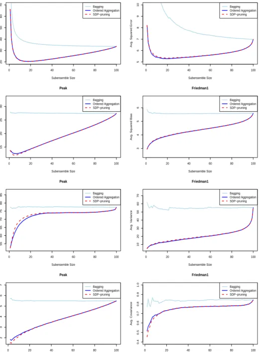
Fig. 4 and Fig. 5 display the average value over the test instances of the squared error, and of its components (squared bias, variance and covariance), as a function of ensemble size for standard bagging, Ordered Aggregation and SDP-pruning for the synthetic regression problemsPeak andFriedman1 and for the real-world problemsPollution and Chick. The characteristics of these problems are displayed in Table 1. In each problem the original bagging en-semble is composed of 100 neural network with 5 units in the hidden layer. These networks are generated on independent bootstrap samples from a fixed
0 20 40 60 80 100 20 30 40 50 60 70 Peak Subensemble Size
Avg. Squared Error
Bagging Ordered Aggregation SDP−pruning 0 20 40 60 80 100 5 6 7 8 9 10 Friedman1 Subensemble Size
Avg. Squared Error
Bagging Ordered Aggregation SDP−pruning 0 20 40 60 80 100 15 20 25 30 Peak Subensemble Size
Avg. Squared Bias
Bagging Ordered Aggregation SDP−pruning 0 20 40 60 80 100 3 4 5 6 Friedman1 Subensemble Size A vg. Squared Bias Bagging Ordered Aggregation SDP−pruning 0 20 40 60 80 100 55 60 65 70 75 80 85 Peak Subensemble Size Avg. Variance Bagging Ordered Aggregation SDP−pruning 0 20 40 60 80 100 10 20 30 40 50 60 70 Friedman1 Subensemble Size A vg. V ar iance Bagging Ordered Aggregation SDP−pruning 0 20 40 60 80 100 2 3 4 5 6 7 Peak Subensemble Size Avg. Covariance Bagging Ordered Aggregation SDP−pruning 0 20 40 60 80 100 0.4 0.5 0.6 0.7 0.8 0.9 1.0 Friedman1 Subensemble Size A vg. Co v ar iance Bagging Ordered Aggregation SDP−pruning
Fig. 4: From top to bottom: average over the test instances of the squared error, squared bias, variance and covariance as a function of ensemble size for bagging, Ordered
0 20 40 60 80 100 3000 5000 7000 9000 Pollution Subensemble Size
Avg. Squared Error
Bagging Ordered Aggregation SDP−pruning 0 20 40 60 80 100 200 400 600 800 1000 Chick Subensemble Size
Avg. Squared Error
Bagging Ordered Aggregation SDP−pruning 0 20 40 60 80 100 2000 3000 4000 5000 6000 Pollution Subensemble Size A vg. Squared Bias Bagging Ordered Aggregation SDP−pruning 0 20 40 60 80 100 100 200 300 400 500 600 Chick Subensemble Size A vg. Squared Bias Bagging Ordered Aggregation SDP−pruning 0 20 40 60 80 100 10000 30000 50000 Pollution Subensemble Size A vg. V ar iance Bagging Ordered Aggregation SDP−pruning 0 20 40 60 80 100 400 600 800 1200 1600 Chick Subensemble Size A vg. V ar iance Bagging Ordered Aggregation SDP−pruning 0 20 40 60 80 100 −100 0 100 200 300 Pollution Subensemble Size A vg. Co v ar iance Bagging Ordered Aggregation SDP−pruning 0 20 40 60 80 100 30 40 50 60 70 80 90 Chick Subensemble Size A vg. Co v ar iance Bagging Ordered Aggregation SDP−pruning
Fig. 5: From top to bottom: average over the test instances of the squared error, squared bias, variance and covariance as a function of ensemble size for bagging, Ordered
training set. In the case of the synthetic problems Peak and Friedman1 the training set is randomly generated and contains 200 instances. The test set is independent of the training data and consists of 2000 elements. In the case of the real-world problems Pollution andChick, sub-sampling is used to carry out the estimations [40]. Specifically, the data are randomly split in a training set and a test set containing 2/3 and 1/3 of the instances, respec-tively. The values of the test error and of its components are estimated by averaging over 1000 realizations of each problem (for Pollution 5000 realiza-tions are used as a consequence of the reduced number of instances available for this problem). The error curves exhibit similar features to those in Fig. 3. For standard bagging, the values of the average squared bias variance and covariance remain approximately constant as the number of regressors in the ensemble varies. In contrast with standard bagging, the average squared bias, variance and covariance typically increase with the size of the subensembles selected using Ordered Aggregation and SDP-pruning. A lower covariance among the ensemble members was also observed in [29] and is a consequence of minimizing (5) [12, 29].
According to (21) and (22), as the size of the ensemble grows, the squared bias and the covariance become the most important terms in the error de-composition. The variance term is inversely proportional tou, the size of the subensemble. Therefore, its contribution to the generalization error becomes smaller as the number of predictors of the ensemble increases. For sufficiently large subensemble sizes the test error of the complete ensemble in standard bagging is approximately equal to the sum of the squared bias and the covari-ance term (23). In consequence, even though the predictors included in the smaller subensembles by SDP-pruning and Ordered Aggregation also have low variance, the main reason for the improvements in performance is that the first regressors incorporated by these strategies have low bias and also small or negative covariance.
3.3. Generalization Performance
In this section we assess the generalization performance of SDP-pruning and Ordered Aggregation and compare these techniques with predictors of different types: a single neural network, bagging, Adaboost.R2, negative correlation learning ensembles (NCL) and regularized stacked generalization combined the lasso (SG-lasso), as described in [43], and the ensemble pruning methods of Perrone and Cooper [39], and GASEN[56]. The experiments are carried out on 24 regression problems from the UCI-Repository [4], from the
Weka Data Mining Tool [52] and from other sources [10, 14, 20, 28, 42]. They include synthetic and real-world problems from different fields of application. Table 1 displays the number of instances, the number of attributes and the source of the different datasets considered.
For each real-world dataset, 10×10-fold cross-validation is used to esti-mate the squared regression error. For the synthetic datasets (Friedman1, Friedman2, Friedman3, and Peak) the values reported are averages over 100 independent realizations of the train and test datasets. The training set and the test set contain 200 and 2000 instances, respectively. Data attributes are normalized so that they have zero mean and unit variance on the training set for each dataset. The computation of the estimates for each training and testing partition involves the following steps: (i) Generate a bagging ensem-ble of 100 neural networks from the training set using bootstrap sampling. The architecture of these neural networks and the weight decay constant used is determined as in Section 3.1. Then, the neural networks are trained over 1000 epochs using the best combination of parameters found. (ii) A single neural network and a boosting ensemble of size 100 are also built using the same network configuration as in the bagging ensemble. The boosting ensem-ble is generated using the Adaboost.R2 algorithm with a linear loss function [18]. A 100 neural network NCL ensemble is generated as described in [29] by training each network during 100 epochs using gradient descent. The weights of the networks are initially set to the values provided by bagging. The λ parameter of the NCL ensemble is set equal to 0.99, as suggested in [12]. Instead of using a fixed value, λ could be determined by cross-validation. However, the results obtained are very similar and do not compensate the increased computational cost. The resulting predictors are then used as a benchmark for performance comparison. (iii) A subensemble of 20 neural net-works (i.e. u= 20) is extracted from the original pool of classifiers generated by bagging using SDP-pruning, as described in Section 2.1. The complete bagging ensemble is then ordered according to Ordered Aggregation and the first 20 regressors of the ordered sequence are selected and aggregated in a pruned subensemble. Additionally, the bagging ensemble is pruned using the technique described by Perrone and Cooper in [39] and using the ge-netic algorithm GASEN introduced in [56]. GASEN is configured to select subensembles of the same size as SDP-pruning and Ordered Aggregation (20 neural networks from the original pool of 100). These pruned predictors are also used as a benchmark for performance comparison. (iv) We also gen-erate a regularized linear stacked generalization ensemble (SG-lasso), where
the coefficients that combine the outputs of the different predictors are es-timated using the lasso, as described in [43]. The initial predictors used in this ensemble method are the 100 neural networks generated in bagging. The regularization parameter of the lasso is selected from a grid of 100 potential values using a nested 10-fold cross-validation to estimate the mean squared error. Only the training data are used to compute this estimate. (v) The error of each method is estimated on the corresponding test set.
Table 2 shows the average mean squared error estimated either by 10× 10-fold cross-validation (real-world problems) or in the test set (synthetic data) for each dataset and each prediction method. The figures displayed are scaled by a factor shown in the first column of the table. The next five columns of the table display the error of a single neural network, the complete bag-ging ensemble, the boosting ensemble, the NCL ensemble and the regular-ized linear stacked generalization ensemble (SG-lasso), respectively. Finally, the four last columns of the table display the average errors of the bagging subensembles selected by SDP-pruning, Ordered Aggregation, the method of Perrone and Cooper and the genetic algorithm GASEN. To determine whether the observed improvements in accuracy are statistically significant a paired Wilcoxon-test [51] is performed, as suggested in [16]. Error values that are significantly better than bagging according to the Wilcoxon text at an α-value of 0.05 are highlighted in boldface. Error values that are signif-icantly worse than bagging are underlined. Similarly, error values that are significantly better than boosting are marked with the symbol ◭. Values
that are significantly worse than boosting are marked with the symbol ⊳.
From these results one can see that bagging ensembles often outperform a single neural network. NCL ensembles and regularized linear stacked gen-eralization ensembles also provide more accurate predictions than bagging or boosting in most of the problems investigated. The subensembles obtained by SDP-pruning and Ordered Aggregation that contain only 20 regressors have a good overall generalization performance in the regression problems investigated. In general, these pruned bagging ensembles outperform sin-gle networks, boosting ensembles and complete bagging ensembles. Table 3 shows that the pruning rates obtained by SDP-pruning and Ordered Ag-gregation (20%) are generally higher than those achieved by the method proposed by Perrone and Cooper (≈ 33 networks on average). Regularized linear stacked generalization ensembles contain an average of ≈ 19 neural networks.
Table 2: Average mean squared error normalized by the corresponding scaling factor. The figures displayed correspond to a single neural network, complete bagging ensembles, Adaboost.R2 ensembles, negative correlation learning (NCL) ensem-bles, regularized linear stacked generalization ensembles (SG-lasso), and pruned bagging ensembles selected by SDP-pruning, Ordered Aggregation (OA), the method of Perrone and Cooper (P&C) and the genetic algorithm GASEN.
Dataset Scaling Neural Net Bagging Adaboost NCL SG-lasso Pruned Bagging
Factor SDP OA P&C GASEN
Attitude ×101 9.45±7.90 8.63±4.95 8.83±4.97 8.59±5.51 8.54±5.92 8.29±5.18◭ 8.29±5.11◭ 8.35±5.55◭ 8.33±5.01◭ AutoPrice ×107 1.17±0.86⊳ 0.74±0.59⊳ 0.56±0.40 0.71±0.58⊳ 0.62±0.47⊳ 0.63±0.50⊳ 0.63±0.50⊳ 0.65±0.50⊳ 0.68±0.51⊳ Bodyfat ×1 2.96±3.76 1.89±2.76◭ 2.55±2.00 2.33±2.66◭ 2.22±2.74◭ 2.12±2.78◭ 2.10±2.78◭ 2.15±2.87◭ 2.01±2.81◭ Bolts ×101 5.31±7.70◭ 6.56±7.69◭ 9.72±13.28 6.07±7.80◭ 4.01±6.26◭ 4.57±7.17◭ 4.50±7.01◭ 4.43±7.21◭ 5.81±7.44◭ Boston ×101 1.27±0.64⊳ 1.15±0.64⊳ 1.00±0.43 1.02±0.57 1.06±0.52 1.07±0.55⊳ 1.07±0.55⊳ 1.10±0.57⊳ 1.13±0.60⊳ Chick ×101 5.44±3.66⊳ 6.57±3.58⊳ 3.89±2.74 3.93±2.40 4.62±2.39⊳ 4.82±2.43⊳ 4.88±2.60⊳ 5.77±3.40⊳ 6.23±3.58⊳ Concrete Slump ×101 3.41±2.15 3.23±1.54 3.12±1.43 2.98±1.45◭ 2.81±1.40◭ 2.85±1.42◭ 2.85±1.44◭ 2.97±1.48◭ 3.16±1.60 Fires ×103 1.82±4.04 1.55±3.49⊳ 1.15±2.59 1.48±3.75 1.62±3.43⊳ 1.32±3.06⊳ 1.31±3.05⊳ 1.58±3.51⊳ 1.63±3.40⊳ Friedman1 ×1 4.82±1.29◭ 4.85±0.44◭ 5.05±0.76 4.34±0.46◭ 4.23±0.53◭ 4.45±0.46◭ 4.45±0.46◭ 4.55±0.48◭ 4.71±0.45◭ Friedman2 ×104 2.68±0.89⊳ 2.19±0.16 2.17±0.13 2.20±0.16 2.02±0.14◭ 2.06±0.14◭ 2.06±0.15◭ 2.06±0.15◭ 2.15±0.15◭ Friedman3 ×10−2 1.83±0.25⊳ 1.70±0.21◭ 1.74±0.22 1.69±0.21◭ 1.69±0.22◭ 1.67±0.22◭ 1.67±0.22◭ 1.68±0.22◭ 1.71±0.22◭ Loblolly ×1 4.45±8.93◭ 6.39±6.36◭ 10.93±9.60 3.95±6.30◭ 4.27±5.65◭ 3.96±6.24◭ 3.93±6.22◭ 3.96±5.91◭ 6.07±8.12◭ Longley ×10−1 8.25±16.10⊳ 13.08±24.85⊳ 5.63±8.13 5.21±5.66 5.14±9.54 4.79±7.82◭ 4.81±7.89◭ 5.20±8.94 10.53±45.79 Orange ×102 2.21±1.80 1.85±1.32 1.97±1.44 1.58±0.83◭ 1.75±1.12 1.68±1.09◭ 1.66±1.06◭ 1.64±1.09◭ 1.70±1.16◭ Ozone ×101 1.69±0.44◭ 1.65±0.43◭ 1.86±0.48 1.65±0.43◭ 1.67±0.46◭ 1.65±0.44◭ 1.65±0.44◭ 1.64±0.43◭ 1.66±0.44◭ Peak ×101 3.16±0.53⊳ 2.63±0.34⊳ 2.47±0.23 1.98±0.28◭ 1.56±0.23◭ 2.37±0.34◭ 2.37±0.34◭ 2.59±0.33⊳ 2.55±0.34⊳ Pollution ×103 5.90±6.54 3.94±3.25 7.50±11.19 2.85±1.71◭ 4.55±9.95◭ 3.25±2.49◭ 3.20±2.47◭ 3.36±4.18◭ 3.47±2.29◭ Rock ×104 8.46±10.24⊳ 6.77±6.81◭ 7.44±7.54 6.82±6.74◭ 7.98±7.83 7.28±7.41 7.25±7.36 7.63±7.56 7.07±7.18◭ Sensory ×10−1 5.34±0.95◭ 5.35±0.92◭ 5.63±0.98 5.28±0.90◭ 5.47±0.91◭ 5.19±0.91◭ 5.20±0.92◭ 5.28±0.92◭ 5.35±0.96◭ Servo ×10−1 3.27±3.28⊳ 2.63±2.35⊳ 1.70±1.78 2.40±2.11⊳ 1.94±1.84⊳ 2.03±1.77⊳ 2.05±1.81⊳ 2.06±1.69⊳ 2.43±2.03⊳ Solder ×1 9.04±3.37◭ 8.36±3.13◭ 9.44±3.53 8.83±3.37◭ 8.48±3.33◭ 8.43±3.23◭ 8.41±3.20◭ 8.33±3.12◭ 8.41±3.14◭ Theoph ×1 5.30±3.77⊳ 4.43±2.27⊳ 3.04±2.15 3.74±2.24⊳ 2.87±1.75 3.42±2.00⊳ 3.41±2.01⊳ 3.25±1.93⊳ 4.11±2.25⊳ 28
Table 3: Average number of networks in the pruned subensembles obtained by the method of Perrone and Cooper (P&C) and in the ensembles generated by regularized linear stacked generalization using the lasso (SG-lasso).
Dataset # of Neural Networks P & C SG-lasso Attitude 16.62±12.94 10.27±2.80 AutoPrice 24.16±7.72 31.43±15.38 Bodyfat 26.87±10.03 20.35±4.24 Bolts 17.20±9.10 12.75±2.75 Boston 52.21±17.35 20.71±8.47 Chick 71.81±10.54 34.78±5.19 Concrete Slump 33.41±14.82 16.97±4.14 Fires 3.19±2.70 11.22±9.12 Friedman1 42.08±13.76 20.80±10.78 Friedman2 23.66±9.82 12.73±2.77 Friedman3 35.52±11.37 15.74±7.00 Loblolly 38.65±18.77 20.19±4.08 Longley 6.80±4.98 8.07±3.22 Orange 23.67±12.34 11.25±3.07 Ozone 35.80±18.16 14.48±5.17 Peak 90.59±6.53 53.71±5.21 Pollution 21.29±17.64 14.79±5.46 Rock 12.56±7.97 8.31±2.64 Sensory 63.64±13.72 28.64±6.47 Servo 36.43±12.82 21.85±10.94 Solder 53.76±11.09 18.62±4.41 Theoph 12.76±14.30 14.77±8.94 Tooth 15.65±8.38 10.05±3.45 Wisconsin 43.72±17.60 19.27±4.78 Average 33.42±21.33 18.82±10.17
the collection of problems investigated can be made using the framework proposed by Demˇsar in [16]. On the basis of the results of Friedman test on the average ranks of each algorithm in the problems investigated, the hypothesis that their performances are equivalent can be rejected atα= 0.05. A Nemenyi test is used to determine whether the differences in average rank among the different algorithms are significant. Fig. 6 displays the results of this test for α = 0.05. In this figure, algorithms whose differences in performance are not statistically significant are linked with a solid black line. Differences in performance between algorithms whose average ranks are further than a critical distance (CD) are statistically significant.
In the collection of regression problems investigated pruned ensembles, regularized linear stacked generalization ensembles and negative correlation learning ensembles have a better overall performance than the correspond-ing complete baggcorrespond-ing ensembles, boostcorrespond-ing ensembles and scorrespond-ingle neural net-works. Notwithstanding, the differences in average rank are only statistically significant for SDP-pruning and Ordered Aggregation. In these problems subensembles selected by Ordered Aggregation or SDP-pruning have better overall generalization performance than the subensembles selected by the method of Perrone and Cooper, SG-lasso and the genetic algorithm GASEN. Furthermore, the differences in the average ranks with respect to this lat-ter method are statistically significant. Ordered Aggregation also performs slightly better than SDP-pruning, although the difference between their av-erage ranks is not statistically significant.
2 3 4 5 6 7 8 Neural Network Bagging Adaboost.R2 GASEN Ordered Aggregation SDP−pruning Perrone & Cooper NCL SG−lasso
CD
Fig. 6: Results of a Nemenyi test on the average ranks of the different regression systems: a single neural network, bagging, boosting (Adaboost.R2), negative correlation learning (NCL), regularized linear stacked generalization (SG-lasso) and pruned subensembles se-lected by SDP-pruning, Ordered Aggregation, the method of Perrone and Cooper and GASEN. The critical difference (CD) between average ranks is displayed at the top of the figure.
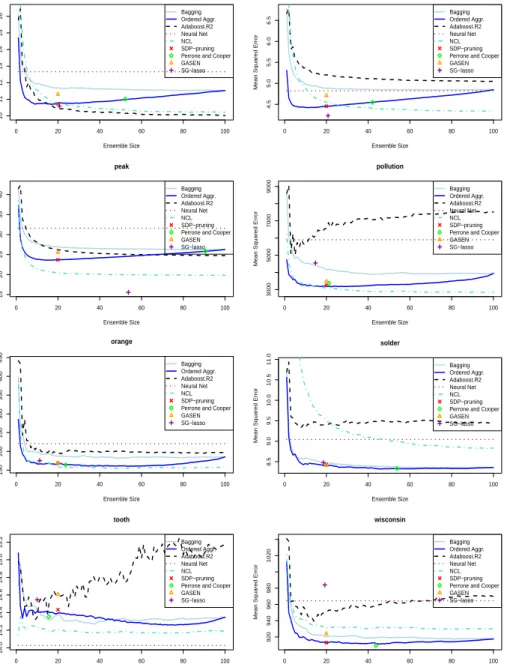
for bagging, Ordered Aggregation, boosting, negative correlation learning (NCL) and regularized linear stacked generalization (SG-lasso) as a function of the ensemble size for a representative subset of the regression problems investigated. For SDP-pruning, because of its high computational cost, only the average error of the subensemble of size u= 20 is displayed. For the ge-netic algorithm GASEN, the method of Perrone and Cooper and regularized linear stacked generalization we display their corresponding mean squared error evaluated at the average number of networks used for prediction. The average error of a single neural network is also marked as a horizontal line for reference. The curves for bagging and Ordered Aggregation exhibit a qualitative behavior that is similar to the curves depicted in Fig. 3. The error decreases almost monotonically as a function of the size of a randomly ordered bagging ensemble. Modifying the order of the aggregation accord-ing to the procedure described leads to an initially steeper descent of the error curves, which, with some exceptions (e.g. Solder, Tooth) is followed by a broad minimum and a final rise to the error level of the complete bag-ging ensemble. In fact, because the error curves are rather flat around the minimum, any value between 15% and 25% percent of the original pool of regressors yields similar results. The performance of the subensembles se-lected by SDP-pruning is similar to the performance of the subensembles obtained by Ordered Aggregation for size u = 20. However, in some cases SDP-pruning leads to slightly higher error rates (e.g. Tooth). The subensem-bles selected by GASEN exhibit in general a higher prediction error than the subensembles selected by either SDP-pruning or Ordered Aggregation. The method of Perrone and Cooper provides better results than those of these two pruning strategies in some problems (e.g.Tooth, Wisconsin). Nevertheless, in several other problems worse results are observed (e.g. Pollution, Peak,
Friedman1, Boston). In particular, the method of Perrone and Cooper tends to underprune and selects subensembles that are too large. Regularized lin-ear stacked generalization (SG-lasso) generates the most accurate ensembles in some problems, e.g. Peak and Friedman1. Nevertheless, the prediction performance of this ensemble method is severely impaired in some cases, e.g.
Wisconsin and Pollution. Finally, NCL provides in general better results than bagging and boosting with a few exceptions (e.g. Solder, Wisconsin). This is in agreement with the findings of [12].
The behavior of boosting ensembles is more erratic, reflecting the lack of robustness of this method. Boosting outperforms bagging, Ordered Aggre-gation and SDP-pruning in a few regression problems (e.g. Boston, Peak).
0 20 40 60 80 100 10 11 12 13 14 15 16 boston Ensemble Size
Mean Squared Error
Bagging Ordered Aggr. Adaboost.R2 Neural Net NCL SDP−pruning Perrone and Cooper GASEN SG−lasso 0 20 40 60 80 100 4.5 5.0 5.5 6.0 6.5 friedman1 Ensemble Size
Mean Squared Error
Bagging Ordered Aggr. Adaboost.R2 Neural Net NCL SDP−pruning Perrone and Cooper GASEN SG−lasso 0 20 40 60 80 100 15 20 25 30 35 40 peak Ensemble Size
Mean Squared Error
Bagging Ordered Aggr. Adaboost.R2 Neural Net NCL SDP−pruning Perrone and Cooper GASEN SG−lasso 0 20 40 60 80 100 3000 5000 7000 9000 pollution Ensemble Size
Mean Squared Error
Bagging Ordered Aggr. Adaboost.R2 Neural Net NCL SDP−pruning Perrone and Cooper GASEN SG−lasso 0 20 40 60 80 100 150 200 250 300 350 400 450 orange Ensemble Size
Mean Squared Error
Bagging Ordered Aggr. Adaboost.R2 Neural Net NCL SDP−pruning Perrone and Cooper GASEN SG−lasso 0 20 40 60 80 100 8.5 9.0 9.5 10.0 10.5 11.0 solder Ensemble Size
Mean Squared Error
Bagging Ordered Aggr. Adaboost.R2 Neural Net NCL SDP−pruning Perrone and Cooper GASEN SG−lasso 0 20 40 60 80 100 14.0 14.2 14.4 14.6 14.8 15.0 15.2 tooth Ensemble Size
Mean Squared Error
Bagging Ordered Aggr. Adaboost.R2 Neural Net NCL SDP−pruning Perrone and Cooper GASEN SG−lasso 0 20 40 60 80 100 920 940 960 980 1020 wisconsin Ensemble Size
Mean Squared Error
Bagging Ordered Aggr. Adaboost.R2 Neural Net NCL SDP−pruning Perrone and Cooper GASEN SG−lasso
Fig. 7: Error curves for standard bagging, Ordered Aggregation, negative correlation learn-ing (NCL) and Adaboost.R2 as a function of the ensemble size for a variety of regression problems. The error of a single Neural Network is displayed as an horizontal line for
ref-erence. The error for a subensemble of size u= 20 selected with SDP-pruning is marked
with a cross. The average error of the method of Perrone and Cooper, the genetic algo-rithm GASEN and regularized linear stacked generalization (SG-lasso) are also displayed at the corresponding average number of selected networks.
However, boosting has a detrimental effect in others (e.g. Tooth, Pollution, Wisconsin). A similar deterioration of performance of boosting has been de-tected in noisy classification problems [17, 35]. The origin of this behavior is that boosting tends to assign larger weights to incorrectly labeled training instances. The learning algorithm is thus forced to reduce the error rate of those instances. This emphasis on examples that are difficult to predict tends to distort the original problem, leading to overfitting and consequently, to a poor generalization performance.
4. Conclusions
Extracting an optimal subensemble from an original regression ensemble is a difficult problem that can be shown to be NP-hard. In this paper we analyze two approximate techniques to address this problem. The first one is based on a Semidefinite Programming relaxation of the original problem. This method is an extension to regression ensembles of the work [55], which introduced SDP-pruning for classification ensembles. The second technique is Ordered Aggregation[26]. This is a forward selection strategy starts with an empty subensemble and incorporates in each step the regressor that reduces the training error of the current subensemble the most. Even though these approximate strategies can lead to suboptimal solutions, a detailed analysis in ensembles of intermediate size shows that the subsets selected have a near-optimal performance and share a large percentage of regressors with near-optimal subensembles obtained by exhaustive search.
The error of standard bagging ensembles typically decreases monotoni-cally as the size of the ensemble is increased. By contrast, for the subsets selected by these techniques, the curves that trace the dependence of the subensemble error as a function of its size show that the minimum error is attained in subensembles of intermediate size. The features of these curves are qualitatively similar for both the training and testing errors. However, the minimum in the test error curves appears at larger sizes than in the curves for the training error. This minimum is generally below the asymp-totic error of the complete bagging ensemble. This means that generalization performance of the ensemble can be improved by retaining only a subset of the regressors generated. A bias-variance-covariance decomposition of the test error shows that the key to the improvements in generalization perfor-mance is the selection of subsets of regressors whose bias is low and whose correlations are small or negative.