Dynamic Programming and Error Estimates for
Stochastic Control Problems with Maximum Cost
Olivier Bokanowski, Athena Picarelli, Hasnaa Zidani
To cite this version:
Olivier Bokanowski, Athena Picarelli, Hasnaa Zidani. Dynamic Programming and Error Esti-mates for Stochastic Control Problems with Maximum Cost. Applied Mathematics and Opti-mization, Springer Verlag (Germany), 2015, 71 (1), pp.125–163. <10.1007/s00245-014-9255-3>.
<hal-00931025v2>
HAL Id: hal-00931025
https://hal.inria.fr/hal-00931025v2
Submitted on 11 May 2014
HAL is a multi-disciplinary open access archive for the deposit and dissemination of sci-entific research documents, whether they are pub-lished or not. The documents may come from teaching and research institutions in France or abroad, or from public or private research centers.
L’archive ouverte pluridisciplinaire HAL, est destin´ee au d´epˆot et `a la diffusion de documents scientifiques de niveau recherche, publi´es ou non, ´emanant des ´etablissements d’enseignement et de recherche fran¸cais ou ´etrangers, des laboratoires publics ou priv´es.
FOR STOCHASTIC CONTROL PROBLEMS WITH MAXIMUM COST
OLIVIER BOKANOWSKI, ATHENA PICARELLI, AND HASNAA ZIDANI Abstract. This work is concerned with stochastic optimal control for a running maximum cost. A direct approach based on dynamic program-ming techniques is studied leading to the characterization of the value function as the unique viscosity solution of a second order Hamilton-Jacobi-Bellman (HJB) equation with an oblique derivative boundary condition. A general numerical scheme is proposed and a convergence result is provided. Error estimates are obtained for the semi-Lagrangian scheme. These results can apply to the case of lookback options in fi-nance. Moreover, optimal control problems with maximum cost arise in the characterization of the reachable sets for a system of controlled sto-chastic differential equations. Some numerical simulations on examples of reachable analysis are included to illustrate our approach.
AMS subject classifications: 49J20, 49L25, 65M15, 35K55
Keywords: Hamilton-Jacobi equations, oblique Neuman boundary condi-tion, error estimate, viscosity nocondi-tion, reachable sets under state constraints, lookback options, maximum cost.
1. Introduction
Consider the controlled processXu
t,x(·)solution of the stochastic differen-tial equation
dX(s) =b(s, X(s), u(s))ds+σ(s, X(s), u(s))dB(s) s∈[t, T]
X(t) =x (1.1)
(whereu∈ U denotes the control process). We are interested in an optimal control problem where the cost function is given by :
J(t, x, u) =E ψ Xt,xu (T), max s∈[t,T]g(X u t,x(s)) , (1.2) and the value function is defined by:
v(t, x) := inf
u∈UJ(t, x, u). (1.3)
Date: May 1, 2014.
This work was partially supported by the EU under the 7th Framework Programme Marie Curie Initial Training Network “FP7-PEOPLE-2010-ITN”, SADCO project, GA number 264735-SADCO.
This problem arises from the study of some path-dependent options in fi-nance (lookback options). Another application of control problem with maximum running cost comes from the characterization of reachable sets for state-constrained controlled stochastic systems (see section 2.3).
The main contributions to the study of this kind of problems can be found in [4] and [11] (see also [26] for the stationary case in the framework of clas-sical solutions). In these works the dynamic programming techniques are applied on the Lp-approximation of theL∞-cost functional (1.2), using the approximation:
a∨b≃(ap+bp)1p (for p→ ∞),
for any a, b ≥ 0, where a∨b := max(a, b). Then a characterization of the auxiliary value functionv (see definition (2.4)) as solution to a suitable Hamilton-Jacobi equation is obtained as limit for p → ∞. A fundamental hypothesis in order to apply this approach is the positivity of the functions involved.
In our work, a direct derivation of a Dynamic Programming Principle for the function v gives an alternative and natural way for dealing with the maximum running cost problems under less restrictive assumptions. By this way, the optimal control problem (1.3) is connected to the solution of a HJB equation with oblique derivative boundary conditions. Here, the boundary conditions have to be understood in the viscosity sense (see [27]).
The second part of the paper is devoted to numerical aspects. First, a general scheme is proposed to deal with HJB equations with oblique deriva-tive boundary conditions. Then, a convergence result is proved by using the general framework of Barles-Souganidis [10] based on the monotonicity, sta-bility, consistency of the scheme (a precise definition of these notions, in the case of HJB equations with oblique derivative boundary condition, is given in section 4.1). Secondly, we focus on the fully discrete semi-Lagrangian scheme and we study some properties of the numerical approximation. Semi-Lagrangian schemes for second order HJB equations (in the general form of Markov chain approximations) have been first considered in the book [32]. In the framework of viscosity solutions, semi-Lagrangian schemes for first order HJB equations have been studied in [20]. Extensions to the second order case can be found in [35, 19, 23, 24]. In our context, the nu-merical scheme that will be studied couples the classical semi-Lagrangian scheme with an additional projection step on the boundary. For this par-ticular scheme, we derive a rate of convergence, generalizing in this way the results already known for general HJB equations without boundary condi-tions. More precisely, an error bound of the order of h1/4 (where h is the time step) is obtained for Lipschitz (unbounded) cost function. The activity related to error estimate for numerical approximations of nonlinear second order degenerate equations dated back few years ago with [30, 31] where some useful techniques of "shaking coefficients" were introduced, and then
mollifiers were used to get smooth sub-solutions. These ideas were later used extensively by many authors [6, 7, 8, 14].
The paper is organized as follows: Section 2 introduces the problem and some motivations. In particular it will be shown how it is possible to con-nect a state-constrained reachability problem to an optimal control problem associated to a cost functional of the form (1.2). Section 3 is devoted to the characterization of the value function by the appropriate HJB equation. A strong comparison principle is also stated. In Section 4 the numerical ap-proximation is discussed and a general convergence result is provided. The semi-Lagrangian scheme is presented in Section 4.2 and the properties of this scheme are investigated. Section 5 focuses on the study of error esti-mates. Finally some numerical tests are presented in Section 6 to analyse the relevance of the proposed scheme.
2. Formulation of the problem
2.1. Setting and preliminary results. Let (Ω,F,P) be a probability space,{Ft, t≥0} a filtration onF andB(·)a Brownian motion inRp (with p≥1).
Given T > 0 and 0 ≤ t ≤ T, the following system of controlled stochastic differential equations (SDEs) inRd (d≥1) is considered
dX(s) =b(s, X(s), u(s))ds+σ(s, X(s), u(s))dB(s) s∈[t, T]
X(t) =x, (2.1)
where u ∈ U set of progressively measurable processes with values in U ⊂ Rm (m ≥ 1), U is assumed to be a compact set. The following classical assumption will be considered on the coefficients band σ:
(H1) b : [0, T]×Rd×U → Rd and σ : [0, T]×Rd ×U → Rd×p are continuous functions. Moreover, there exist Lb, Lσ >0such that for everyx, y∈Rd, t∈[0, T], u∈U:
|b(t, x, u)−b(t, y, u)| ≤Lb|x−y|, |σ(t, x, u)−σ(t, y, u)| ≤Lσ|x−y|. We recall some classical results on (2.1) (see [39]):
Theorem 2.1. Under assumption (H1) there exists a unique Ft-adapted
process, denoted by Xt,xu (·), strong solution of (2.1). Moreover there exists a constant C0 >0, such that for anyu∈ U, 0≤t≤t′ ≤T andx, x′ ∈Rd
E " sup θ∈[t,t′] Xt,xu (θ)−Xt,xu ′(θ) 2 # ≤ C02|x−x′|2, (2.2a) E " sup θ∈[t,t′] Xt,xu (θ)−Xtu′,x(θ) 2 # ≤ C02(1 +|x|2) |t−t′|, (2.2b) E " sup θ∈[t,t′] Xt,xu (θ)−x2 # ≤ C02(1 +|x|2) |t−t′|. (2.2c)
Consider two functions ψ, g such that:
(H2) ψ : Rd×R → R and g : Rd → R are Lipschitz functions. Their Lipschitz constants will be denoted by Lψ and Lg respectively. In this paper we deal with optimal control problems of the form
v(t, x) := inf u∈UE ψ Xt,xu (T), max s∈[t,T]g(X u t,x(s)) . (2.3)
Under assumptions (H1) and (H2), v is a Lipschitz continuous function in x and a 12-Hölder continuous function in t (by the same arguments as in Proposition 2.2 below). In order to characterize the functionv as solution of an HJB equation the main tool is the well-known optimality principle. The particular non-Markovian structure of the cost functional in (2.3) prohibits the direct use of the standard techniques. To avoid this difficulty it is classical to reformulate the problem by adding a new variable y ∈ R that, roughly speaking, keeps the information of the running maximum. For this reason, we introduce an auxiliary value functionϑ defined on[0, T]×Rd×Rby:
ϑ(t, x, y) := inf u∈UE ψ Xt,xu (T), max s∈[t,T]g(X u t,x(s))∨y . (2.4) The following property holds:
ϑ(t, x, g(x)) =v(t, x), (2.5) so from now on, we will only work with the value function ϑsince the value of vcan be obtained by (2.5) .
Proposition 2.2. Under assumptions (H1) and (H2), ϑ is a Lipschitz con-tinuous function in (x, y) uniformly with respect to t, and a 12-Hölder con-tinuous function in t. More precisely, there exists Lϑ>0 (Lϑ depends only
on C0, Lψ, Lg) such that:
|ϑ(t, x, y)−ϑ(t′, x′, y′)| ≤Lϑ(|x−x′|+|y−y′|+ (1 +|x|)|t−t′|
1 2),
for all (x, y),(x′, y′)∈Rd+1 and for anyt≤t′ ∈[0, T].
Proof. Let be t≤t′ ≤T and x, x′ ∈Rd. Notice that the following property holds for the maximum
|(a∨b)−(c∨d)| ≤ |a−c| ∨ |b−d|. Then, the inequalities (2.2) yield to:
ϑ(t, x, y)−ϑ(t, x′, y)≤Ksup u∈U E " sup s∈[t,T] Xt,xu (s)−Xt,xu ′(s) # ≤KC0|x−x′|
for K=Lψ(Lg+ 1). In a similar way, we obtain ϑ(t, x, y)−ϑ(t′, x, y) ≤ Lψsup u∈U E " Xt,xu (T)−Xtu′,x(T) +Lg sup s∈[t,t′] Xt,xu (s)−x+ +Lg sup s∈[t′,T] Xtu′,x(s)−Xtu′,Xu t,x(t′)(s) # ≤ K′(1 +|x|)t−t′ 1 2
for a positive constant K′ > 0 that depends only on Lψ, Lg and C0. The Lψ-Lipschitz behavior in the variableyis immediate. We conclude then the
result withLϑ=K∨K′∨Lψ.
2.2. Summary of the main results. The first important theoretical result is contained in Theorem 3.2 where it is established that ϑ is a viscosity solution (in the sense of Definition 3.3) of the following HJB equation with oblique derivative boundary conditions
−∂tϑ+H(t, x, Dxϑ, D2xϑ) = 0 in[0, T)×D −∂yϑ= 0 on[0, T)×∂D ϑ(T, x, y) =ψ(x, y) inD (2.6) for a suitable choice of the domain D⊂Rd+1.
Theorem 3.4 states a comparison principle for (2.6), adapting the result of [25] to parabolic equations in unbounded domains. Thanks to this result, ϑ is finally characterized as the unique continuous viscosity solution of the HJB equation.
Starting from Section 4 the numerical aspects will be discussed. A numer-ical scheme for the approximation ofϑwill be proposed. Theorem 4.1 gives a general convergence result under hypotheses of stability, consistency and monotonicity.
Error estimates for the semi-discrete semi-Lagrangian scheme are inves-tigated in the Theorems 5.4 and 5.5, while the rate of convergence for the fully discrete scheme is given in Theorem 5.6.
2.3. Motivations.
Reachability for state constrained control systems. A first motiva-tion comes from the reachability analysis for state-constrained stochastic controlled systems. Let C ⊆ Rd be a target set, and let K ⊆ Rd be a set of state constraints. Let dC (resp. dK) denotes the Euclidean distance func-tions fromC(resp. K). The aim is to characterize and compute the backward reachable setRCt,K defined by
RCt,K := x∈Rd, ∀ε >0, ∃uε∈ U such that E[dC(X uε t,x(T))]≤εandE[ max s∈[t,T]dK(X uε t,x(s))]≤ε .
Remark 2.3. Straightforward calculations yield to the following formulation: RCt,K≡ x∈Rd,∀ε >0,∃uε ∈ U, E[dC(X uε t,x(T))∨ max s∈[t,T]dK(X uε t,x(s))]≤ε . (2.7) Indeed, this is easily deduced from the following inequalities:
E dC(Xt,xuε(T)) ∨E max s∈[t,T]dK(X uε t,x(s)) ≤E dC(Xt,xuε(T))∨ max s∈[t,T]dK(X uε t,x(s)) ≤E dC(Xt,xuε(T)) +E max s∈[t,T]dK(X uε t,x(s)) . Many works in the literature have been devoted to the reachability anal-ysis for general stochastic controlled systems, we refer to [2, 3]. Stochastic target problems arising in finance have been also analysed [37, 17]. Here, we suggest to characterize the reachable sets by using the level set approach introduced by Osher and Sethian in [36] in the deterministic case. At the basis of this approach there is the idea of considering the setRCt,K as a level set of a continuous function defined as the value function of a suitable op-timal control problem. Recently, the level-set approach has been extended to deal with general deterministic optimal control problems in presence of state constraints, see for example [12, 1]. The level set approach can be also extended to the stochastic setting by considering the following optimal control problem: v(t, x) := inf u∈UE dC(X u t,x(T))∨ max s∈[t,T]dK(X u t,x(s)) . (2.8)
Then the following equivalence can easily be proved
Theorem 2.4. Under assumption (H1), for everyt≥0, we have:
x∈ RCt,K⇐⇒v(t, x) = 0. (2.9)
Proof. The result follows immediately from Remark 2.3. In view of Theorem 2.4, the reachable set RCt,K can be characterized by means of the value function of a control problem with supremum cost in the form of (2.3), with functions g and ψ defined by: g(x) := dK(x) and ψ(x, y) :=dC(x)∨y.
Lookback options in finance. Another interest for computing expectation of supremum cost functionals is the lookback options in Finance. The value of such an option is typically of the form
e v(t, x) =E e−RtTr(s)dsψ XT, max θ∈[t,T]g(Xθ)) ,
whereXθ (the "asset") is a solution of a one-dimensional SDE (2.1),g(x) = x, r(·) is the interest rate, and ψ is the payoff function. Here the option value depends not only on the value of the asset at time T but also on all
the values taken between timestandT. A detailed description of this model can be found in [38]. Typical payoff functions areψ(x, y) =y−x(lookback floating strike put), ψ(x, y) = max(y −E,0) (fixed strike lookback call), ψ(x, y) = max(min(y, E)−x,0)(lookback limited-risk put), etc., see [38, 5] (see also [4] for other examples and related american lookback options).
3. The HJB equation
In all the sequel, we will use the abbreviationa.s. foralmost surely. Also,
almost every will be abbreviated as a.e.. The abbreviation usc (resp. lsc) will be used for upper semi-continuous (resp. lower semi-continuous). 3.1. Dynamic Programming. The aim of this section is to characterize the value function ϑdefined by (2.4) as the unique viscosity solution of an HJB equation. Let us define the process
Yt,x,yu (θ) := max
s∈[t,θ]g(X u
t,x(s))∨y, (3.1) then the optimal control problem (2.4) can be re-written as
ϑ(t, x, y) := inf
u∈UE
ψ Xt,xu (T), Yt,x,yu (T). (3.2) Stochastic optimal control problems with running maximum cost in the vis-cosity solutions framework have been studied in [4, 11]. The arguments developed in that papers are based on the approximation technique of the L∞-norm and they only apply if ψ and g are positive functions. Here, we derive the HJB equation directly without using any approximation. For this, the first step is the Bellman’s principle that we state in the following theorem.
Theorem 3.1 (Dynamic Programming Principle). Under hypothesis (H1) and (H2), for all(t, x)∈[0, T)×Rdand all family of stopping times{θu, u∈ U}
independent of Ft with values on [t, T]: ϑ(t, x, y) = inf
u∈UE
ϑ(θu, Xt,xu (θu), Yt,x,yu (θu)). (3.3) A proof of Theorem 3.1 can be obtained by adapting the same arguments developed by Bouchard and Touzi in [18], thanks to the fact that the couple of variables(Xt,xu (·), Yt,x,yu (·))satisfies the following fundamental property
Xt,xu (s) Yt,x,yu (s) = X u θ,Xu t,x(θ)(s) Yθ,Xu u t,x(θ),Yt,x,yu (θ)(s) ! a.s.
for any stopping time θ with t ≤ θ ≤ s ≤ T. In our case the proof is even simpler than the one of [18] thanks to the uniform continuity of ϑ (Proposition 2.2).
3.2. Hamilton-Jacobi-Bellman equation. Theorem 3.1 is the main tool for proving next result that characterizesϑ as a solution, in viscosity sense, of a HJB equation with oblique derivative boundary conditions. Set
D:=n(x, y)∈Rd+1|y≥g(x)o=Epigraph(g), (3.4) whereDis the interior of D.
Theorem 3.2. Under assumptions (H1) and (H2), ϑ is a continuous vis-cosity solution of the following HJB equation
−∂tϑ+H(t, x, Dxϑ, D2xϑ) = 0 in [0, T)×D (3.5a) −∂yϑ= 0 on [0, T)×∂D (3.5b) ϑ(T, x, y) =ψ(x, y) in D (3.5c) with H(t, x, p, Q) := sup u∈U −b(t, x, u)p−1 2T r[σσ T](t, x, u)Q. (3.6)
(In all the paperDx,Dx2 denote respectively the first and second order
deriva-tives with respect tox.)
Before starting the proof we recall the definition of viscosity solution for problem (3.5) (see [21] and the references therein for a complete discussion on weak boundary conditions).
Definition 3.3. A usc function ϑ (resp. lsc function ϑ) on [0, T]×D is a viscosity sub-solution (resp. super-solution) of (3.5), if for each function ϕ ∈ C1,2([0, T]×D), at each maximum (resp. minimum) point (t, x, y) of ϑ−ϕ(resp. ϑ−ϕ) the following inequalities hold
−∂tϕ+H(t, x, Dxϕ, Dx2ϕ)≤0 in[0, T)×D min −∂tϕ+H(t, x, Dxϕ, D2xϕ),−∂yϕ≤0 on [0, T)×∂D min ϑ−ψ,−∂tϕ+H(t, x, Dxϕ, Dx2ϕ),−∂yϕ≤0 on {T} ×∂D min ϑ−ψ,−∂tϕ+H(t, x, Dxϕ, D2xϕ) ≤0 on {T} ×D. (3.7) (resp. −∂tϕ+H(t, x, Dxϕ, Dx2ϕ)≥0 in[0, T)×D max −∂tϕ+H(t, x, Dxϕ, Dx2ϕ),−∂yϕ≥0 on[0, T)×∂D max ϑ−ψ,−∂tϕ+H(t, x, Dxϕ, Dx2ϕ),−∂yϕ≥0 on{T} ×∂D max ϑ−ψ,−∂tϕ+H(t, x, Dxϕ, D2xϕ) ≥0 on{T} ×D.) (3.8) Finally a continuous functionϑis a viscosity solution of (3.5) if it is both a sub- and a super-solution.
Proof of Theorem 3.2. First, from the definition of ϑ, we obtain easily that ϑ(T, x, y) =ψ(x, y).
Now, we check thatϑis a viscosity sub-solution. Letϕ∈C1,2([0, T]×D) such that ϑ−ϕattains a maximum at point (¯t,x,¯ y¯)∈[0, T)×D. Without
loss of generality we can always assume that(¯t,x,¯ y¯)is a strict local maximum point (let us say in a ball of radiusr >0centered in(¯t,x,¯ y¯)) andϑ(¯t,x,¯ y¯) =
ϕ(¯t,x,¯ y¯). Thanks to Theorem 3.1, for any u ∈ U and for any sufficiently small stopping time θ=θu, we have:
ϕ(¯t,x,¯ y¯) =ϑ(¯t,x,¯ y¯)≤E[ϑ(θ, X¯t,¯ux(θ), Y¯t,¯ux,¯y(θ))]
≤E[ϕ(θ, X¯t,¯ux(θ), Y¯t,¯ux,¯y(θ))]. (3.9) Two cases will be considered depending on if the point(¯x,y¯) belongs or not to the boundary of D.
- Case 1: g(¯x)<y¯. Consider a constant control u(s) ≡u∈U. From the continuity of g and the a.s. continuity of the sample paths it follows that, for a.e. ω∈Ω, there existss¯(ω)>¯tsuch thatg(Xt,¯¯ux(s))<y¯if s∈[¯t,s¯(ω)). Let beh >0, and letθ¯be a the following stopping time:
¯ θ:= infs >¯t|(Xu ¯ t,¯x(s), Y¯t,ux,¯y¯(s))∈/Br(¯x,y¯) ∧(¯t+h)∧inf s >t¯|g(Xu ¯ t,x¯(s))≥y¯ , (3.10)
(here and through the paperBr(x0)denotes the ball of radiusr >0centered at x0). One can easily observe that a.s. Y¯t,¯ux,¯y(¯θ) = ¯y, then by (3.9)
ϕ(¯t,x,¯ y¯)≤E[ϕ(¯θ, Xt,¯¯ux(¯θ),y¯)] ∀u∈U.
By applying the Ito’s formula, and thanks to the smoothness of ϕ, we get: E "Z θ¯ ¯ t − ∂tϕ−b(s, X¯t,¯ux(s), u)Dxϕ− 1 2T r[σσ T](s, Xu ¯ t,¯x(s), u)D2xϕds # ≤0. Since the stopping times
infns >¯t|(Xt,¯¯ux(s), Yt,¯¯ux,¯y(s))∈/ Br(¯x,y¯) o
and infns >¯t|g(Xt,¯¯ux(s))≥y¯ o are a.s. strictly greather than ¯t, it follows that a.s. θ¯−¯t >0. Therefore, E " 1 ¯ θ−¯t Z θ¯ ¯ t − ∂tϕ−b(s, X¯t,¯ux(s), u)Dxϕ− 1 2T r[σσ T](s, Xu ¯ t,¯x(s), u)D2xϕds # ≤0. By the dominate convergence theorem and the mean value theorem, letting h going to 0, it follows −∂tϕ−b(¯t,x, u¯ )Dxϕ−1 2T r[σσ T](¯t,x, u¯ )D2 xϕ≤0, ∀u∈U, and finally: −∂tϕ+ sup u∈U −b(¯t,x, u¯ )Dxϕ− 1 2T r[σσ T](¯t,x, u¯ )D2 xϕ ≤0.
- Case 2: g(¯x) = ¯y. Assume that−∂yϕ(¯t,x,¯ y¯)>0, otherwise the conclu-sion is straightforward. Consider a constant control u(s) ≡u∈U. Thanks to the continuity of the sample paths and the smoothness of ϕ, for a.e. ω there is a time ¯s(ω)>¯tand η >0 such that:
Letθ¯be the stopping time given by: ¯ θ:= infns >¯t|(Xt,¯¯ux(s), Yt,¯¯ux,¯y(s))∈/ Br(¯x,y¯) o ∧infns >t¯|g(X¯t,¯ux(s))∈/ [¯y,y¯+η) o ∧infns >t¯|∂yϕ(s, Xt,¯¯ux(s),y¯)≥0 o ∧(¯t+h). By (3.9) one has ϕ(¯t,x,¯ y¯)≤E[ϕ(¯θ, Xt,¯¯ux(¯θ),y¯)], which implies: −∂tϕ+ sup u∈U −b(¯t,x, u¯ )Dϕ− 1 2T r[σσ T](¯t,x, u¯ )D2ϕ ≤0. In conclusion, min −∂tϕ+ sup u∈U −b(¯t,x, u¯ )Dϕ−1 2T r[σσ T](¯t,x, u¯ )D2ϕ, −∂yϕ ≤0, and ϑis a viscosity sub-solution of equation (3.5).
It remains to prove that ϑ is a viscosity super-solution of (3.5). Let ϕ∈C1,2([0, T]×D)be such thatϑ−ϕattains a minimum at point(¯t,x,¯ y¯)∈ [0, T)×D. Without loss of generality we can always assume that (¯t,x,¯ y¯) is a strict local minimum point andϑ(¯t,x,¯ y¯) =ϕ(¯t,x,¯ y¯). Thanks to the DPP, for any sufficiently small stopping time θ=θu one has
ϕ(¯t,x,¯ y¯) =ϑ(¯t,x,¯ y¯) = inf u∈UE[ϑ(θ, X u ¯ t,¯x(θ), Y¯t,¯ux,¯y(θ))] ≥ inf u∈UE[ϕ(θ, X u ¯ t,¯x(θ), Y¯t,¯ux,¯y(θ))].
This can be treated by using again the same arguments as for the sub-solution
proof.
3.3. Comparison principle. The section is concluded with a compari-son principle for equation (3.5). There is a large literature dealing with Neumann-type or oblique derivative boundary conditions. We refer to [34, 9] for the first order case and to [29, 28] for second order equations. For dealing with this kind of problems some regularity assumption on the domain D is often required. In our case the definition ofDis strictly connected with the choice of the function g that is, without further hypothesis, only Lipschitz continuous. The result below has the advantage of taking into account also this non smooth case.
Theorem 3.4. Assume that (H1)-(H2) are satisfied. Let ϑ(resp. ϑ) a usc (resp. lsc) viscosity sub-solution (resp. super-solution) of (3.5) satisfying the following growth condition (forC >0):
ϑ(t, x, y) ≤ C(1 +|x|+|y|),
(resp. ϑ(t, x, y) ≥ −C(1 +|x|+|y|).
Such a comparison principle is proved in [25] for elliptic equations in bounded domains. The arguments extend the ones used in [29, 28] for the case when the domain D has a smooth boundary. For convenience of the reader we give the main steps of the proof in Appendix A, and show how the arguments can be adapted for the parabolic case in unbounded domains. Assertions of Theorems 3.2 and 3.4 lead to the following result:
Corollary 3.5. Under assumptions (H1) and (H2), the value function ϑis the unique continuous, Lipschitz in (x,y), viscosity solution of equation (3.5)
on [0, T]×D.
The uniqueness result is stated onD, which means that the solution to the HJB equation coincides with the value function ϑ on [0, T]×D. Then ϑis extended in a unique way on[0, T]×Rd×Rby: ϑ(t, x, y) =ϑ(t, x, y∨g(x)).
4. Numerical approximation
Now, we focus on general approximation schemes for (3.5). LetN ≥1be an integer (number of time steps), and let
h:= T
N, and tn:=nh,
for n= 0, . . . , N. Let ∆x = (∆x1, . . . ,∆xd) ∈(R∗+)dbe a mesh step in Rd,
∆y >0be a mesh step inR, andρ:= (h,∆x,∆y)be a set of mesh steps (in time and space).
For a givenρ, consider the corresponding space grid Gρ:=
n
(xi, yj) = (i∆x, j∆y),for (i, j)∈Zd×Z o
.
where for i∈Zd, i∆x := (i1∆x1,· · ·, iN∆xN). For any x∈Rd, let jx ∈Z be the upper integer part of g(x)∆y, i.e,
jx:= minj ∈Z, j∆y≥g(x) .
Consider aprojectionoperator (along the directioney)ΠGρdefined as follows:
ΠGρ(Φ)(t n, xi, yj) := Φ(tn, xi, yj), ∀j ≥jxi, i∈Z d, Φ(tn, xi, yjxi), ∀j < jxi, i∈Z d, for any Φ∈C([0, T]×Rd×R,R).
We aim at computing an approximationWi,jn of the value function ϑ(tn, xi, yj), on the grid Gρ. ByWρ, we will denote the interpolation of the valuesWi,jn at (tn, xi, yj). The valuesWi,jn are defined recusively as follows:
General scheme (GS)
2)Forn=N, . . . ,1, the valueWi,jn−1 is obtained as solution of:
Sρ(tn−1, xi, yj, Wi,jn−1,ΠGρ(Wρ)) = 0, ∀i, j withg(xi)≤yj, (4.1) Wi,jn−1 :=Wi,jn−1
xi, ∀i, j withg(xi)> yj, (4.2)
whereSρ: [0, T]×D×R×C([0, T]×Rd×R,R)→Ris a scheme operator. Typical operatorSρcan be obtained by using an explicit or implicit finite difference method on (3.5a) (see [16, 15, 33]), or a semi-Lagrangian (SL) scheme ([35, 19, 24]). In (4.1), the value ofWi,jn−1 may depend on the whole function Wρ (i.e., all the values Wi,jk for k= 0,· · ·, N). Of course, in case of an explicit time discretization, the step (4.1) could be re-written as:
Sρ(tn−1, xi, yj, Wi,jn−1,ΠGρ(Wρ(tn,·,·))) = 0, ∀i, j withg(xi)≤yj. However, the formulation (4.1) is more general and includes different kind of time-discretization like Euler implicit scheme orθ-methods.
The main idea of the numerical method described here above is to mix the use of a standard scheme for (3.5a), together with a "projection step" on ∂D in order to approximate the homogeneous oblique derivative boundary condition (3.5b). Let us point out that a similar method was introduced in [5] for the caseg(x)≡ |x|. However, the general case with possibly nonlinear function g requires some further attention on the boundary.
4.1. A general convergence result. In this part we closely follow the arguments of Barles and Souganidis [10], using consistency, stability and monotonicity arguments. For this, we assume that the following hypotheses are considered:
(H3) (stability) For any ρ, there exists a solutionWρof the scheme which has linear growth (uniformly in ρ), that is, there exists a constant C >0, independent of ρ, such that
|Wρ(t, x, y)| ≤C(1 +|x|+|y|), on [0, T]×D; (4.3) (H4) (consistency) The scheme Sρ is consistent with respect to equation (3.5a) in [0, T]×D, that is, for all(t, x, y)∈[0, T]×Dand for every
Φ∈C1,2([0, T]×D), lim ρ→0 [0,T]×D∋(s,ξ,γ)→(t,x,y) ζ→0 Sρ(s, ξ, γ,Φ(s, ξ, γ)+ζ,Φ +ζ) =−∂tΦ+H(t, x, DxΦ, D2xΦ).
(H5) (monotonicity) For anyρ, forr∈R,(t, x, y)∈[0, T]×D,Sρ(t, x, y, r,Φ) depends only on the values of Φ in a neighborhood Bη(ρ)(t, x, y) of
(t, x, y), with η(ρ) ≥ 0 such that η(ρ) −→ρ→0 0. Moreover, for any
Φ1,Φ2 functions on [0, T]×Rd×R → R, such that Φ1 ≥ Φ2 on Bη(ρ)((t, x, y)), it holds:
Let us point out that the monotonicity and the consistency are required here only for the operator scheme Sρ that corresponds to the discretization of the equation−∂tϑ+H(t, x, Dϑ, D2ϑ) = 0.
Notice also that the monotonicity assumption (H5) is slightly different from the classical one usualy required for general HJB equations. The reason for this comes from the fact that the operator schemeSρis defined onDand may use some values of the functionWρoutside the domain Dthat are ob-tained by oblique projection through the projection step. Our monotonicity assumption requires local dependency on the values of Φin a neighborhood of the point under consideration, then a comparison of the scheme values is requested for any two functionsΦ1 and Φ2 such that Φ1 ≥Φ2 only on this neighborhood. The proof of Theorem 4.1 highlights what this requirement is needed for.
In the next section, we will check that assumptions (H3)-(H5) are well satisfied by the semi-Lagrangian scheme. Now, we state the convergence result for any general scheme satisfying (H3)-(H5).
Theorem 4.1. Assume (H1)-(H2). Let Sρ be a scheme satisfying (H3)-(H5). Then, whenρtends to0,Wρconverges to the unique viscosity solution
of (3.5) uniformly on each compact subset of[0, T]×D. Proof. Let us define
W(t, x, y) := lim sup
[0,T]×D∋(s,ξ,γ)→(t,x,y) ρ→0
Wρ(s, ξ, γ)
and W(t, x, y) := lim inf
[0,T]×D∋(s,ξ,γ)→(t,x,y) ρ→0
Wρ(s, ξ, γ).
We start by proving thatW is a viscosity sub-solution of equation (3.5) (the proof that W is a viscosity super-solution is analogous).
Letϕbe inC1,2([0, T]×D)and let(¯t,x,¯ y¯)be a local maximum point for W −ϕon[0, T]×D. Without loss of generality we can assume that(¯t,x,¯ y¯)
is a strict local maximum in the restricted ballBr(¯t,x,¯ y¯)∩([0, T]×D) for a certain r >0,
(W −ϕ)(¯t,x,¯ y¯) = max
Br∩([0,T]×D)
(W −ϕ) = 0, and ϕ≥2 supρkWρk∞ outside the ball B
r(¯t,x,¯ y¯). We first assume that¯t∈(0, T). Then we claim that:
−∂tϕ+H(¯t,x, D¯ xϕ, Dx2ϕ)≤0 if(¯x,y¯)∈D, (4.4a) or min −∂tϕ+H(¯t,x, D¯ xϕ, Dx2ϕ),−∂yϕ≤0 if (¯x,y¯)∈∂D.(4.4b) Following [21], there exists a sequence of mesh steps ρk and a sequence
k→+∞, and (tk−1, xk, yk) is a global maximum point of Wρk−ϕ, with (Wρk−ϕ)(t k−1, xk, yk) = max [0,T]×D (Wρk−ϕ) =δ k k−→→∞0 (4.5) and Wρk(t k−1, xk, yk)k−→→∞W(¯t,x,¯ y¯).
- Case 1: assume that y > g¯ (¯x). Thus, (¯x,y¯) is in the open set D and for k large enough, (xk, yk) ∈ D. By continuity of g, y > g(x) in Bη(ρk)(tk−1, xk, yk) for ρk small enough. Therefore ΠGρ(Wρk) = Wρk ≤ ϕ+ δk on Bη(ρk)(tk−1, xk, yk). On the other hand, W
ρk(t
k−1, xk, yk) = ϕ(tk−1, xk, yk) +δk. Hence, thanks to the monotonicity of the scheme, it follows
0 = Sρk(t
k−1, xk, yk, Wρk(tk−1, xk, yk),ΠGρ(Wρk)) ≥ Sρk(t
k−1, xk, yk, ϕ(tk−1, xk, yk) +δk, ϕ+δk).
Using the consistency of the scheme, we obtain in the limit whenρk→0, −∂tϕ+H(¯t,x, D¯ xϕ, D2xϕ)≤0. (4.6) We conclude that (4.4a) is satisfied when (¯x,y¯)∈D.
- Case 2: wheny¯=g(¯x),(xk, yk)can be also on ∂Dand the scheme may involve values Wkℓn on some points (xk, yℓ) that are not inD. Here, we need to consider two sub-cases.
- Sub-Case 2.1: if −∂yϕ(¯t,x,¯ y¯)≤0, then (4.4b) holds.
- Sub-Case 2.2: if −∂yϕ(¯t,x,¯ y¯) >0, then there exists a neighborhood V of (¯t,x,¯ y¯) where ∂yϕ(t, x, y) is well defined, and −∂yϕ(t, x, y)>0for every
(t, x, y)∈ V. Therefore,
y≤y′ =⇒ϕ(t, x, y)≥ϕ(t, x, y′) ∀(t, x, y),(t, x, y′)∈ V. (4.7) Forklarge enough,Bη(ρk)(tk−1, xk, yk)⊂ V. Let(t, x, y)∈Bη(ρk)(tk−1, xk, yk).
Ify≥g(x), then ΠGρ(Wρk(t, x, y)) =Wρk(t, x, y)≤ϕ(t, x, y) +δ k. (4.8) Otherwise if y < g(x),ΠGρ(Wρk(t, x, y)) =Wρk(t, x, y jx), and we have ΠGρ(Wρk(t, x, y)) = Wρk(t, x, y jx) ≤ ϕ(t, x, yjx) +δk (by using (4.5)) (4.9) ≤ ϕ(t, x, y) +δk (by using (4.7)) (4.10) (for (4.10) we also used the continuity of g that ensures that for k big enough (t, x, yjx) still lays in V). We conclude Π
Gρ(Wρk) ≤ ϕ+ δ
k on Bη(ρk)(tk−1, xk, yk). Thus by monotonicity (H5), we get
0 = Sρk(t
k−1, xk, yk, Wρk(tk−1, xk, yk),ΠGρ(Wρk)) ≥ Sρk(t
k−1, xk, yk, ϕ(tk−1, xk, yk) +δk, ϕ+δk). Using the consistency of the scheme, when ρk→0, we get
As conclusion for case 2, (4.4b) is satisfied when(¯x,y¯)∈∂D.
Similar arguments can be used in order to treat the case ¯t=T (classical arguments enable to treat also the case of the boundary¯t= 0). We conclude thatW is a viscosity sub-solution of the equation (3.5).
As already mentioned, we can also show thatW is a super-solution. Then by the comparison principle on[0, T]×D(Theorem 3.4 and using the growth condition (4.3)), the inequality W ≥ W holds on [0, T]×D. Furthermore since the reverse inequality W ≤ W is always true, we deduce that W =
W =ϑon[0, T]×D. Hence the convergence result is proved. 4.2. A semi-Lagrangian scheme. We first introduce some new notations: for any u ∈ U, the drift b(·,·, u) (resp. volatility σ(·,·, u)) will be simply denoted bybu (resp. σu).
Consider the operatorT :C(Rd+1)→C([0, T]×Rd+1) defined by: T(φ)(t, x, y) = min u∈U 1 2p 2p X k=1 φxx+hbu(t, x)+php(−1)kσu ⌊k+1 2 ⌋ (t, x), y(4.12) where(σuk)k=1,...,p are the column vectors ofσu, and⌊q⌋ denotes the integer part of q. The notation [·] ≡ [·]x stands for a monotone, P1 interpolation operator on thex-grid(xi), satisfying for every Lipschitz continuous function φ(with Lipschitz constant Lφ):
(i) [φ]x(xi) =φ(xi),∀i, (ii)|[φ]x(x)−φ(x)| ≤Lφ|∆x|, (iii) |[φ]x(x)−φ(x)| ≤C|∆x|2kDx2φk∞ if φ∈C2(Rd),
(iv) for any functions φ1, φ2 :Rd→R,φ1≤φ2 ⇒ [φ1]x≤[φ2]x. (4.13)
The operatorT corresponds to a discretisation of the equation (3.5a) by a semi-Lagrangian scheme (see [35, 19, 24]). Now, define an approximation method for the system (3.5) as follows:
Fully discrete scheme (FDS)
1)Initialisation step: for all i, j, set Wi,jN =ψ(xi, yj∨g(xi)). 2)Forn=N, . . . ,1:
- Step 1 Compute Wn−
1 2
i,j = T(W·n,·)(tn, xi, yj), for all i, j (here W·n,· denotes the values {Wi,jn |i, j ∈Zd×Z});
- Step 2 ComputeWi,jn−1= ΠGρ
(Wn−12), for all i, j.
The FDS scheme is a particular GS method, with the following formula for the operator Sρ: Sρ(t−h, x, y, r,Φ) := 1 h r−ΠGρ(T(Φ)(t, x, y)) . (4.14)
Remark 4.2. We point out that in the FDS, for j such that yj < g(xi), the projection step fixes the value of Wi,jn−1 as Wi,jn−1
xi. Of course, other
1)Initialization step: for n=N, for all i, j, set WfN
i,j =ψ(xi, yj∨g(xi)). 2)Forn=N, . . . ,1,Wfi,jn−1=Te(Wf·n,·)(tn, xi, yj), for alli, j, where
e T(φ)(t, x, y) = min u∈U 1 2p 2p X k=1 φx,y x+hbu(t,x)+php(−1)kσ⌊uk+1 2 ⌋ (t,x), y∨g(x), with[·]x,y standing for an interpolation in both variablesx and y.
All the convergence results stated in the paper also hold for this new scheme.
In the next subsection, we will study some properties of the approximated solution Wρ. Before this, we define also the following semi-discrete scheme where we consider only a time-discretization:
Semi-discrete scheme (SDS)
1)Forn=N, for every(x, y)∈Rd+1, setVN(x, y) =ψ(x, y∨g(x)). 2)Forn=N, . . . ,1, defineVn−1 as the function defined by:
Vn−1(x, y) =T0(Vn)(tn, x, y∨g(x)), (4.15) where,T0 is defined fromC(Rd+1) intoC([0, T]×Rd+1) by:
T0(φ)(t, x, y) := min u∈U 1 2p 2p X k=1 φx+hbu(t, x) + (−1)kphpσu ⌊k+12 ⌋ (t, x), y. Unlike the fully discrete scheme, no interpolation step is required in the SDS. Straightforward calculations lead to the following consistency estimate, for any φ∈C2,4((0, T)×Rd×R): 1 h(φ(t−h, x, y)− T0(φ)(t, x, y))− −∂tφ+H(t, x, Dxφ, D2xφ) (4.16) ≤ K1max u∈U k∂tt2φk∞+|bu(t, x)|2kD2xφk∞+|bu(t, x)||σu(t, x)|2kD3xφk∞ +|σu(t, x)|4kD4xφk∞ h,
for any(x, y)∈Rd, withK1a positive constant independent ofφ. Moreover, T andT0 satisfy the following properties :
Lemma 4.3. For every φ1, φ2 ∈C([0, T]×Rd×R), we have:
(i) (T0(φ1)− T0(φ2))+≤ k(φ1−φ2)+k;
(ii) kTφ1− Tφ2k∞≤ kφ1−φ2k∞;
(iii) kT0φ1− T0φ2k∞≤ kφ1−φ2k∞;
(iv) for any Lipschitz continuous function φon Rd×R,kTφ− T0φk∞≤ Lφ∆x, whereLφ is a Lipschitz constant of φ.
Notice that assertion (i) corresponds to a discrete comparison principle. The proof of the lemma is straightforward and will be omitted.
4.3. Convergence of the SL scheme. The aim of this subsection is to prove a convergence result for the scheme FDS.
Theorem 4.4. Let assumptions (H1)-(H2) be satisfied. Let Wρ be defined by the fully discrete scheme. Assume also that
|(∆x,∆y)|
h ≤C (where C is a positive constant) (4.17)
Then the FDS is convergent, i.e. Wρ converges towards ϑ, as ρ tends to 0,
uniformly on each compact set of [0, T]×D.
The claim of this theorem would be a consequence of the general result of theorem 4.1, provided the monotonicity, consistency and stability properties of the FDS are established. The monotonicity and the consistency are easy to check. If ψ is a bounded function, the stability of the scheme would be immediate because in this case kWnk∞ ≤ kψk∞. However, in the general case the functionψis not necessarily bounded. In order to derive the stability property, we first prove some results on the semi-discrete scheme that we state in the following next two propositions.
Proposition 4.5. If assumptions (H1) and (H2) are satisfied, the solution
V of the semi-discrete scheme is Lipschitz continuous in(x, y)and 12-Hölder continuous in t: there exists a constant LV ≥ 0, for every 0 ≤ n, m ≤ N,
and every(x1, y1),(x2, y2)∈Rd+1 such that
|Vn(x2, y2)−Vm(x1, y1)| ≤LV |x2−x1|+|y2−y1|+ (1 +|x1|)|tn−tm|1/2.
Proof. Let(ξn, ξn+1, . . . , ξN−1), be independent random variables, with val-ues in{0, . . . ,2p}, and such that P(ξn=k) = 2p1, ∀k= 1, . . . ,2p.
Letu= (un, un+1, . . . , uN−1)denotes a sequence of controls, withui ∈U, and letZkn=Zkn,x,u,n≤k≤N, be the random walk such that:
( Znn=x, Zk+1n =Zkn+hbuk(t k+1, Zkn) + √ hσ¯uk ξk(tk+1, Zkn), k≥n (4.18)
where the notation σ¯ku(t, x) := (−1)k√pσu ⌊k+1
2 ⌋
(t, x) is used. Notice that Zkn,x,u depends only on the controls (un, . . . , uk−1). Direct calculations lead to the following expressions:
Vn(x, y) = min un∈U 1 2p 2p X k=1 Vn+1 x+hbun(t n+1, x) + √ hσ¯un k (tn, x), y∨g(x) = min un∈U E Vn+1 Zn+1n,x,u, y∨g(x) ,
and, in the same way, Vn(x, y) = min un∈U E min un+1∈U EVn+2(Zn+1,Z n,x,u n+1 ,u n+2 , y∨g(x)∨g(Zn+1n,x,u)) , = min un∈UE min un+1∈U EVn+2(Zn+2n,x,u, y∨g(x)∨g(Zn+1n,x,u)) , and so on, and finally (also usingVN(x, y)≡ψ(x, y∨g(x))):
Vn(x, y) =min un E min un+1E · · ·min uN−1E VN ZNn,x,u, y∨ max i=n,...,N−1g(Z n,x,u i ) · · · =min un E min un+1E · · ·min uN−1E ψ ZNn,x,u, y∨ max i=n,...,Ng(Z n,x,u i ) · · · . Then, we have the equivalent representation formula:
Vn(x, y) = min u=(un,...,uN−1) E ψ(ZNn,x,u, y∨ max i=n,...,Ng(Z n,x,u i )) . (4.19) By using|(x2∨y2)−(x1∨y1)| ≤ |x1−x2| ∨ |y1−y2| ≤ |x1−x2|+|y1−y2|, we obtain: |Vn(x2, y2)−Vn(x1, y1)| ≤ ≤Lψmax u E |Zn,x2,u N −Z n,x1,u N |+Lg max n≤i≤N|Z n,x2,u i −Z n,x1,u i |+Lg|y2−y1| ≤Lψ(Lg+ 1) max u E max n≤i≤N|Z n,x2,u i −Z n,x1,u i | +|y2−y1| , (4.20) where max
u denotes the maximum over (un, un+1, . . . , uN−1) ∈ U
N−n. By (H1), there exists a constant C1 ≥0, that depends only on (T, Lσ, Lb), such that for every0≤m, n≤N and everyx, x1, x2 ∈Rd, the following classical estimates hold: E max n≤i≤N Zn,x2,u i −Z n,x1,u i ≤ C1|x2−x1| (4.21a) E max 0≤i≤p
Zm+in,x,u−Zmn,x,u
≤ C1|tm+p−tm|1/2(1 +|x|).(4.21b) Combining (4.20) and (4.21a), forn=m, the Lipschitz property follows:
|Vn(x1, y1)−Vn(x2, y2)| ≤Lψ(Lg+ 1)(C1|x2−x1|+|y2−y1|). On the other hand, for 0≤n≤m≤N by using again (4.19) we have: |Vm(x, y)−Vn(x, y)| ≤Cmax u E max n≤i≤NZ n,x,u i −mmax≤i≤NZ m,x,u i .(4.22)
for some constantC. Therefore, since Zmm,x,u=x: |Vm(x, y)−Vn(x, y)| ≤ Cmax u E max n≤i≤mZ n,x,u i −x (4.23) +Cmax u E max m+1≤i≤NZ n,x,u i −m+1max≤i≤NZ m,x,u i .(4.24) The right term of (4.23) is bounded by C(1 +|x|)|tm −tn|1/2. In order to bound (4.24), by using that Zin,x,u = Zm,Zmn,x,u,u
i (∀i ≥m) and (4.21a) the following estimate is obtained:
E max m+1≤i≤NZ m,Zmn,x,u,u i −m+1max≤i≤NZim,x,u ≤ C1EZmn,x,u−x ≤ C12(1 +|x|)|tm−tn|1/2. Hence it holds, for some constant C,
|Vn(x, y)−Vm(x, y)| ≤C(1 +|x|)|tm−tn|1/2.
Together with the Lipschitz property the desired result follows.
Remark 4.6. It is not clear whether the solution Wρ obtained by the fully discrete scheme satisfies a Lipschitz continuity property or not. The main difficulty is that a representation formula as (4.19) is not guaranteed forWρ. Proposition 4.7. If assumptions (H1) and (H2) are satisfied, there exists a constant C >0 independent of ρ such that, ∀n= 0, . . . , N:
kWn−Vnk∞≤C|(∆x,∆y)|
h . (4.25)
Proof. Consider the operator Π : C(Rd ×R) → C(Rd ×R) defined by
Πφ(x, y) =φ(x, y∨g(x)). With this notation, we have Vn−1 = Π(T0(Vn)). On the other hand, Wijn−1 = ΠGρ
(T(Wn)(t n, xi, yj)). Therefore, by using Lemma 4.3, we get: kWn−1−Vn−1k∞≤ kΠGρ(T(Wn))−Π(T0(Vn))k∞ ≤ kΠGρ(T(Wn))−ΠGρ(T0(Vn))k∞+kΠG ρ (T0(Vn))−Π(T0(Vn))k∞ ≤ kT(Wn)−T0(Vn)k∞+kΠG ρ (T0(Vn))−Π(T0(Vn))k∞ ≤ kT(Wn)−T(Vn)k∞+kT(Vn)−T0(Vn)k∞+LV∆y ≤ kWn−Vnk∞+LV|∆x|+LV∆y. By recursion, it follows: kWn−Vnk∞ ≤ kWN−VNk∞+nLV(|∆x|+ ∆y). Since VN(x, y) =ψ(x, y∨g(x)) onRd+1,WN is an interpolation of VN on the gridGρ and n≤ T
h, we obtain the desired result. Now we turn to the proof of Theorem 4.4.
Proof of Theorem 4.4. SinceVnis a Lipschitz function in the(x, y)variables, uniformly in n, thenVn has a linear growth with constants independent of n. By Lemma 4.7, and by using assumption (4.17),
kWn−Vnk∞≤C|(∆x,∆y)|
h ≤K.
HenceWn has also a linear growth, with constants independent ofn. Moreover, the consistency of the scheme comes from the estimate (4.16) and using that |∆xh|2 → 0 by assumption (4.17). Also, the monotonicity property (as defined in (H5)) is deduced from the monotonicity of the inter-polations and the monotonicity of the operatorT0.
In consequence, the convergence result follows from Theorem 4.1.
Remark 4.8. The convergence result of Theorem 4.4 is still valid in the case whereψ is a bounded Lipschitz function and |∆xh|2 →0.
5. Error bounds for the semi-Lagrangian scheme
In the sequel, for any functionf defined from some setQ⊂(0,∞)×Rd+1 into eitherR,Rd or some space of matrices, we set
[f]1 := sup (t,x)6=(s,y) |f(t, x)−f(s, y)| (|x−y|+|t−s|1/2), and |f|1:=kfk∞+ [f]1.
In this section we aim to give an error bound for the fully discrete scheme FDS, as well as the semi-discrete SL scheme (4.15). For this aim a supple-mentary hypothesis will be required (together with (H1) and (H2)):
(H1’) There is a constant M1 independent of u∈ U such that: |σu|1+|bu|1 ≤M1.
The error estimates theory is based on some technique of "shaking coeffi-cients" and regularization introduced by Krylov in [30, 31] and studied later by many authors [6, 7, 8, 13, 14, 24]. The main idea consists of regularizing the exact solutionϑin order to obtain a smooth sub-solutionϑε (for an ap-proximation parameter ε >0) to the equation (3.5), then the upper-bound error estimate can be obtained by using the consistency estimate (4.16). The regularisation procedure takes advantage from the fact that the exact solu-tionϑis Hölder continuous, which enables to obtain an estimate of|ϑ−ϑε|∞ of orderO(ε). The lower bound is obtained by similar arguments, but in this case we need to build a smooth sub-solution to the discrete equation. For this, a regularization of the numerical solution will be considered. However, as noticed earlier (remark 4.6), it is not clear if the solution Wρ of the fully discrete scheme is Hölder continuous or not, and then it is not clear how to build directly a regularizationWερ(with regularisation parameterε) with an error|Wρ−Wερ|of order O(ε). For this reason, we will start by deriving an
error estimate between the solutionϑand the solutionV of the semi-discrete scheme SDS, using the fact that V has Hölder continuity properties. Then the estimates for the FDS are derived as a consequence of Lemma 4.7.
For the regularization procedure, consider a smooth function µ:Rd+2 → R, withµ≥0, supported in(0,1)×B1(0), withRRRRdµ(s, x)dxds= 1, and
defineµε as the following sequence of mollifiers: µε(t, x, y) := 1 εd+3µ( t ε2, x ε, y ε) inR×R d+1.
5.1. The rate of convergence for the semi-discrete scheme. For any ε >0, letE be the set of progressively measurable processes(α, χ) valued in
[−ε2,0]×B(0, ε)⊂R×Rdthat is,
E:=prog. meas. process(α, χ) valued inE , whereE :=n(a, e)∈R×Rd,−ε2 ≤a≤0,|e| ≤εo.
On other hand, let M := 2q1 +L2
g and introduce gε :Rd → Rdefined by
gε(x) :=g(x)−M ε. (5.1) Finally, let us denote by Dε the set defined as follows:
Dε:=n(x, y)∈Rd+1, y > gε(x) o
.
Remark 5.1. The choice of gε is such that the following property holds:
(x, y)∈D=⇒(x−e1, y−e2)∈Dε ∀(e1, e2)∈Rd+1,|(e1, e2)| ≤ε.
5.1.1. Upper bound. Now, we start by introducing a perturbed control prob-lem (with "shaking coefficients"). For anyε >0, consider the following value function ϑε(t, x, y) := inf u∈U, (α,χ)∈E E ψ Xt,xu,(α,χ)(T), max s∈[t,T]gε(X u,(α,χ) t,x (s))∨y , (5.2)
whereXt,xu,(α,χ)(·) is the solution of the perturbed system of SDEs
dX(s) =b(s+α(s),X(s) +χ(s),u(s))ds+σ(s+α(s),X(s)+χ(s),u(s))dB(s)
X(t) =x.
(5.3)
Remark 5.2. The functionsσ andbare only defined for times t∈[0, T], but they can be extended to times[−2ε2, T+ 2ε2]in such a way that assumption (H1’) still holds.
Proposition 5.3. Under assumptions (H1)-(H2) and (H1’) (extending even-tually b and σ as prescribed in Remark 5.2), the following holds:
(i) ϑε is a Lipschitz continuous function in x and y and a 12-Hölder continuous function in t. More precisely, for t,≤t′ ∈[0, T], x, x′ ∈ Rd and y, y′ ∈R, we have:
|ϑε(t, x, y)−ϑε(t′, x′, y′)| ≤Lϑ(|x−x′|+|y−y′|+ (1 +|x|)|t−t′|
1 2).
(ii) |ϑ(t, x, y)−ϑε(t, x, y)| ≤Cεon[0, T]×D, where the constantC only
depends on T and the Lipschitz constants of b, σ, g andψ.
Proof. The Lipschitz and Hölder continuity follows by the same arguments as in Proposition 2.2. Thanks to the Lipschitz continuity ofψandgand the choice of gε one has
|ϑ(t, x, y)−ϑε(t, x, y)| ≤K sup u∈U, (α,χ)∈E E " sup s∈[t,T] Xt,xu (s)−Xt,xu,(α,χ)(s) # +M ε
and the result is obtained by classical estimates thanks to the hypothesis on
band σ.
Theorem 5.4. Let assumptions (H1)-(H2) and (H1’) be satisfied. There exists a constant C ≥0 such that
ϑ(tn, x, y)−Vn(x, y)≤C h
1 4,
for all n≥0 (with nh≤T) and (x, y)∈D. Proof. The proof is splitted into three steps:
- Step 1. Let (˜a,(˜e1,˜e2)) ∈ R×Rd+1 be such that −ε2 ≤ ˜a ≤ 0 and |(˜e1,e˜2)| ≤ε. Let (¯t,x,¯ y¯)∈(0, T)×D, and define for ν >0:
Iν(¯t,x,¯ y¯) :=(t, x, y)|t∈[¯t−ν2,t¯],(x, y)∈Bν(¯x,y¯) . We claim that ϑε(· −˜a,· −e˜1,· −e˜2)is a viscosity sub-solution of
−∂tϑ+H(t, x, Dxϑ, Dx2ϑ)≤0 on Iε(¯t,x,¯ y¯). (5.4) To prove this claim, we notice first that Iε(¯t,x,¯ y¯) ⊂ Dε. Moreover, from Theorem 3.2, for anyε >0,ϑεis a viscosity solution of the following equation
−∂tϑε+ sup (a,e)∈E H(t+a, x+e, Dxϑε, D2xϑε) = 0 (−2ε2, T)×Dε, −∂yϑε= 0 (−2ε2, T)×∂Dε, ϑε(T, x, y) =ψ(x,(g(x)−M ε)∨y). (5.5) Letϕ∈C2,4([−2ε2, T]×Dε)be such thatϑε(· −˜a,· −˜e
1,· −˜e2)−ϕachieves a local maximum at (˜t,x,˜ y˜) on Iε(¯t,x,¯ y¯). Clearly (˜t−˜a,x˜−˜e1,y˜−e˜2) is also a local maximum of ϑε−ϕ(·+ ˜a,·+ ˜e
1,·+ ˜e2) on I2ε (andI2ε ⊂Dε). Sinceϑε is a viscosity solution of equation (5.5), we obtain:
−∂tϕ(˜t,x,˜ y˜) + sup (a,e1)∈E
H(˜t−˜a+a,x˜−e˜1+e1, Dxϕ, D2xϕ)≤0. Taking(a, e1) = (˜a,˜e1), we get the result.
- Step 2. Define following mollification ϑε: ϑε(t, x, y) := (ϑε∗µε)(t, x, y) = Z |(e1,e2)|≤ε −ε2 ≤a≤0 ϑε(t−a, x−e1, y−e2)µ(a, e1, e2)dade. We recall the following properties of the mollifiers:
|ϑε(t, x, y)−ϑε(t, x, y)| ≤[ϑε]1ε, (5.6) with[wǫ]1 ≤CLϑ,C ≥0. Moreover, for any i≥1 orj ≥1,
kDxiϑεk∞≤CLϑε1−i, kDtjϑεk∞≤CLϑε1−2j (5.7) (where Dxi denotes the i-th derivative with respect to x, and Dtj the j-th derivative with respect to t). Since ϑε is a limit of convex combinations of ϑε(· −˜a,· −˜e1,· −e˜2), thenϑε satisfies in the viscosity sense
−∂tϑε+H(t, x, Dxϑε, D2xϑε)≤0 in(0, T)×D. (5.8) Taking into account thatϑε is inC∞([0, T]×Rd+1), we conclude that (5.8) holds in classical sense on[0, T]×D. From the consistency estimate (4.16) along with (5.8) and by assumption (H1’), we get:
ϑε(tn−1, x, y)− T0(ϑε)(tn, x, y)≤ C h2 ε3. Combining these bounds with Lemma 4.3, we get
ϑε(tn−1, x, y)−Vn−1(x, y) ≤ T0(ϑε)(tn, x, y)− T0(Vn)(x, y) +Ch 2 ε3 ≤ k ϑε(tn,·)−Vn+k∞+C h2 ε3. Therefore, by recursion, it comes
k(ϑε(tn,·)−Vn)+k∞≤ k(ϑε(0,·)−VN))+k∞+CT h
ε3. (5.9) -Step 3. By Proposition 5.3 together with the inequalities (5.6) and (5.9), we obtain forn≥0,
k(ϑ(tn,·)−Vn)+k∞≤Cε+CT h
ε3, n≥0. The choice ε4 =h leads to (for n≥0):
k(ϑ(tn,·)−Vn)+k∞≤C h
1 4,
5.1.2. Lower bound. For obtaining the lower bound we will apply exactly the same techniques as used for the upper bound, reversing the role of the equation and the scheme. The key point is that the solutionV of the semi-discrete scheme SDS is Lipschitz continuous. Then it is possible to use the techniques of "shaking coefficients" and regularisation to build a smooth sub-solutionVε satisying kVεn−Vnk∞≤Cεand
Vεn−1(x, y)− T0(Vεn)(tn, x, y∨g(x))≤0 in[0, T]×Rd×R. Then by consistency estimate and comparison principle, we conclude the following result:
Theorem 5.5. Let assumptions (H1)-(H2) and (H1’) be satisfied. There exists a constant C >0 such that
ϑ(tn, x, y)−Vn(x, y)≥ −C h
1 4
for all n≥0 (with N h≤T) and (x, y)∈D.
5.2. The fully discrete scheme. The section is concluded with the fol-lowing theorem that provides error estimates for the fully discrete semi-Lagrangian scheme. The result is a simple consequence of Theorems 5.4, 5.5 and Lemma 4.7.
Theorem 5.6. Let assumptions (H1)-(H2) and (H1’) be satisfied. If W is the solution of the fully-discrete scheme (4.14), there exists a constantC >0
independent fromn= 0, . . . , N such that
kWn−ϑ(tn,·)k∞≤C h14 +|(∆x,∆y)| h .
Proof. The result follows by using
kWn−ϑ(tn,·)k∞≤ kWn−Vnk∞+kVn−ϑ(tn,·)k∞.
and thanks to Theorems 5.4, 5.5 and to Lemma 4.7. 6. Numerical tests
In this section we present some numerical results for reachability problems in presence of state constraints (as in Section 3). The dynamics is given by the following controlled SDE inR2:
dX(s) =u(s) 1 0 ds+u(s)σ(X(s))dBs, s≥t, X(t) =x (6.1) whereB is a one-dimensional Brownian motion (p= 1),U = [0,1]⊂R and the function σ(x)∈R2 will vary depending on the example. The target set is
C=x≡(x1, x2)∈R2, 0≤x1≤0.4, |x2| ≤0.5 and the set of state-constraints is
Given a final time T, the aim is to approximate the set RCt,K defined by (2.7), fort= 0. We recall that the following auxiliary value is introduced:
ϑ(t, x, y) = inf u∈UE dC(X u t,x(T))∨ max s∈[t,T]dK(X u t,x(s))∨y and that the characterization of the backward reachable set is given by
x∈ RCt,K⇐⇒ϑ(t, x,0) = 0. (6.2) In all the following tests,t= 0,T = 0.5 are fixed and the computational domain for (x1, x2, y) is
(x1, x2, y)∈Ω = [−1,1]×[−1,1]×[0,1].
The numerical scheme implemented is the semi-Lagrangian scheme (FDS). We denote by Nt the number of time-steps, Nx1 = Nx2 and Ny are the
number of mesh steps for the space variables(x1, x2, y), and h:= T Nt , ∆xi = 2 Nxi , ∆y= 1 Ny .
Different simulations show that the results are not very sensitive to the step discretization of the variabley. Unless otherwise precised, we setNy =
10. For all tests, since u∈[0,1]and because the dynamics depends linearly on the control u it is sufficient to take only two controls (Nu = 2), e.g., u∈ {0,1} for the discretization of the control variable.
The different figures (see e.g. Figure 1) represent points in the (x1, x2) plane. The obstacle is represented in black, and the target in dark grey. Then, an arbitrary non negative threshold ǫ := 10−5 is choosen, and our approximation of the reachable set is given by
e RCt,K:= (x1, x2)∈R2, ϑ(0, x1, x2, ǫ)≤ǫ (6.3) (plotted in green).
Remark 6.1. This procedure is not very sensitive to the choice of ǫ in the range10−2−10−6.
Remark 6.2. We have also tested the scheme of Remark 4.2 and obtain similar results.
Test 1. In this test, there is no diffusion, that is: σ(x) := 0 0 .
Figure 1(a) shows the approximation obtained using(Nx1, Nx2, Nt) = (800,800,200)
(and the represented level set is10−5).
The boundary ofRCt,K (resp. ReCt,K) is also represented by a black doted line (resp. red line). The result perfectly matches the expected solution.
(a) (b)
Figure 1. (a): Test 1, no diffusion, and (b): Test 2, with diffusion.
Test 2. In this test a non-zero volatility is considered: σ(x) :=
0 5
In that case the backward reachable set reduces to the target set, see Fig-ure 1(b). In fact for any point outside the target, as soon as u 6= 0, even if the drift steers the system in the direction of the target, there is always a non-zero probability to go to far way in the x2 orthogonal direction and therefore to not reach it.
Test 3. In this test the volatility is now given by σ(x) = 5dΘ(x)
0 1
wheredΘ denotes the distance function to the set
Θ :=(x1, x2), |x2| ≥0.3 .
Hence for any point (x1, x2), if|x2| ≥0.3 the volatility vanishes. According to the drift term, the target is finally reached, see Figure 2. This Figure shows the approximation of RCt,K for three different meshes. It also shows how the scheme converges. Notice that the points which are immediately above or below the obstacle are not in the reachable set since in presence of diffusion the state-constraint will be violated with a non-zero probability.
Also, in Table 1, various error norms are given to study the convergence of the scheme. For a given n≥1 we have chosen
Nx1 =Nx2 =n, Nt=n/4 and Ny =n/4.
Errors have been computed by taking n = 160 for the reference value, and a convergence of order greater than one is observed in this simple example (better than the expected order of convergence).
Figure 2. (Test 3) Vertical diffusion, using
(Nx1, Nx2, Nt) = (n, n, n/4), for n∈ {200,400,800}.
Table 1. Test 3, convergence table.
n L∞-error order L1-error order L2-error order
10 0.46582 - 0.02526 - 0.07115
-20 0.16633 1.48 0.00345 2.87 0.01979 1.84
40 0.06746 1.30 0.00111 1.63 0.00668 1.56
80 0.02500 1.43 0.00024 2.20 0.00194 1.78
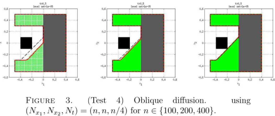
Test 4 (oblique diffusion) In this test the coefficient σ is now given by σ(x) = 5dΘ(x) 1 1 (6.4) In Figure 3 we have plotted the results obtained with three different meshes, using(Nx1, Nx2, Nt) = (n, n, n/4)for n∈ {100,200,400}. Altough
the first computation plotted in Figure 3 (left, with n = 100) is not very accurate, the other computations (with n= 200 andn= 400) clearly show the good convergence of the scheme.
Figure 3. (Test 4) Oblique diffusion. using
Appendix A. Proof of the Comparison principle
In what follows we consider a general HJB equation with oblique derivative boundary condition in the directionν possibly depending onx:
wt+H(t, x, Dw, D2w) = 0 (0, T)×D hν(x), Dwi= 0 (0, T)×∂D w(0, x) =w0(x) D (A.1)
whereD,ν :Rn →Rn,H: [0, T]×Rn×Rn×Sn (Sn is the space of n×n symmetric matrices), and w0:Rn→Rsatisfy the following properties:
(P1) Dis a locally compact subset ofRnsuch that there existsb >0such that [ 0≤t≤b Btb(x+tν(x))⊂Dc, ∀x∈∂D, [ 0≤t≤b Btb(x−tν(x))⊂D, ∀x∈∂D;
(P2) H ∈ C(R×D×Rn ×Sn) and there is a neighborhood U of ∂D in D and a function ω1 ∈ C([0,∞]) satisfying ω1(0) = 0 such that ∀t∈[0, T), x∈U, p, q∈Rn, X, Y ∈ Sd
|H(t, x, p, X)− H(t, x, q, Y)| ≤ω1(|p−q|+kX−Yk);
(P3) There is a function ω2 ∈C([0,∞])satisfying ω2(0) = 0such that H(t, y, p,−Y)− H(t, x, p, X)≤ω2(α|x−y|2+|x−y|(|p|+ 1)) ∀α ≥1, t∈[0, T), x, y ∈D, p∈Rn, X, Y ∈ Sn such that −α I 0 0 I ≤ X 0 0 Y ≤α I −I −I I .
(P4) ν is C2(Rn) ∩W2,∞(Rn) with |ν(x)| = 1, and w0 is a Lipschitiz continuous function.
It is clear that under assumption (H1)-(H2), equation (3.5) is a particu-lar case of (A.1), with n = d+ 1, D ≡ Epigraph(g), ν ≡ −ey, H(t,·) ≡ H(T −t,·). We notice also that under (H1)-(H2), the set defined by D =
Epigraph(g) satisfies the property (P1), with b:= 1/q1 +L2
g. The proper-ties (P2)-(P4) are also satisfied under (H1)-(H2).
In the sequel, it will be usefull to use the concept of semijets:
Definition A.1 (Parabolic semijets). Let O be a locally compact subset of Rn. We define the parabolic semijets of a function w : [0, T]× O → R in
(t, x)∈(0, T)× O by: P1,2,+w(t, x) := (a, p, X) ∈R×Rn× Sn|as(0, T)× O ∋(s, y)→(t, x) w(s, y)≤w(t, x) +a(s−t) +hp, y−xi+1 2hX(y−x),(y−x)i +o(|s−t|+|y−x|2) P1,2,−w(t, x) := (a, p, X)∈R×Rn× S n|as(0, T)× O ∋(s, y)→(t, x) w(s, y)≥w(t, x) +a(s−t) +hp, y−xi+1 2hX(y−x),(y−x)i +o(|s−t|+|y−x|2) . Then we define the closures of the previous sets:
P1,2,+w(t, x) := (a, p, X)∈R×Rn× Sn|∃(tk, xk, ak, pk, Xk)such that (ak, pk, Xk)∈ P1,2,+w(tk, xk)and (tk, xk, w(tk, xk), pk, Xk)→(t, x, w(t, x), p, X) P1,2,− w(t, x) := (a, p, X)∈R×Rn× S n|∃(tk, xk, ak, pk, Xk)such that (ak, pk, Xk)∈ P1,2,−w(tk, xk)and (tk, xk, w(tk, xk), pk, Xk)→(t, x, w(t, x), p, X)
Theorem A.2. Assume (P1)-(P4) hold. Let u (resp. v) be a usc sub-solution (resp. lsc super-sub-solution) of (A.1) satisfying the following growth conditions
u(t, x) ≤ C(1 +|x|),
(resp. v(t, x) ≥ −C(1 +|x|)).
Thenu≤v on [0, T]×D.
Before starting the proof we state some important preliminary results. Lemma A.3. If (P1) and (P4) hold, then there exists a family {wε}ε>0 of C2 functions on Rn×Rn and positive constantsθ, C such that
ϑε(x, x) ≤ ε (A.2) ϑε(x, y) ≥ θ| x−y|2 ε (A.3) hν(x), Dxϑε(x, y)i ≥ −C|x−y| 2 ε if y−x /∈Γ (A.4) hν(x), Dyϑε(x, y)i ≥ 0 if x−y /∈Γ (A.5) |Dyϑε(x, y)| ≤ C| x−y| ε , (A.6) |Dxϑε(x, y) +Dyϑε(x, y)| ≤ C| x−y|2 ε (A.7) and D2ϑε(x, y)≤C 1 ε I −I −I I +|x−y| 2 ε I2d (A.8) for ε >0 and x, y∈Rn.
Lemma A.4. If (P1) and (P4) hold, then there exists h∈C2(D)such that:
h≥0 on D and h= 0 inD\U
(whereU is a neighborhood of ∂D as in Property (P2)) and
hν(x), Dh(x)i ≥1 x∈∂D.
Proof. The result can be obtained adapting the arguments in [25], thanks to
the local compactness of the set D.
Proof of Theorem A.2. We will prove the theorem for u and v sub- and super-solution of (A.1) with boundary condition respectively replaced by hν(x), Dui+α and hν(x), Dvi −α for a certain α > 0. It means that on
(0, T)×∂D,uand v satisfy
min (hν(x), pi+α , a+H(t, x, p, X))≤0 ∀(a, p, X)∈ P1,2,+u(t, x) (A.9) max (hν(y), qi −α , b+H(t, y, q, Y))≥0 ∀(b, q, Y)∈ P1,2,−
v(t, y). (A.10)
We observe that it is always possible to consider a sub-solutionuγ such that (
lim
t→Tuγ(t, x) =−∞
∂t(uγ) +H(t, x, Duγ, D2uγ)<0
defining, for instance, uγ(t, x) := u(t, x) − Tγ−t. The desired comparison result is then obtained as a limit for γ →0.
Givenδ >0, let us defineρδ:= sup (t,x)∈[0,T)×D
u(t, x)−v(t, x)−2δ(1 +|x|2). The growth condition onuandvimplies that there exists(s, z)∈[0, T)×D such that ρδ=u(s, z)−v(s, z)−2δ(1 +|z|2). Setρ:= lim δ→0ρδ.Assumeρ≤0. Sinceu(t, x)−v(t, x)≤2δ(1 +|x| 2) +ρ δ,for every(t, x)∈[0, T)×D, we have that u(t, x)≤v(t, x) on[0, T)×D.
Now, assume thatρ >0and let us show a contradiction. Thanks to (P1) and (P4), ifz∈∂D, then there existsδ∈(0,12)such thatBtδ(x+tν(z))⊂Dc for x∈Bδ(z)∩∂D, t∈(0,2δ]. Set Γ := S
t>0
Btδ(tν(z))◦. It comes that y−x /∈Γ, if x∈∂D∩Bδ(z)◦, y∈D∩Bδ(z)◦. (A.11) In what follows we will restrict our attention to the events on the setBδ(z)∩ D, then we can assumeν ∈W2,∞(Rn,Rn) and |ν(x)|= 1.
Thanks to Lemma A.3 we can define
Φ(t, x, y) :=u(t, x)−v(t, y)−α|x−z|2−ϑε(x, y)−δ(1 +|x|2)−δ(1 +|y|2). and thanks to the growth conditions and the semicontinuity ofuandvwe can state that there exists (¯t,x,¯ y¯) ∈[0, T)×D maximum point for Φ. Thanks to (A.2) and (A.3) the following inequalities hold
ρδ−ε≤Φ(s, z, z)≤Φ(¯t,x,¯ y¯) (A.12) ≤u(¯t,x¯)−v(¯t,y¯)−α|x¯−z|2 −θ|x¯−y¯| 2 ε −δ(1 +|x¯| 2 )−δ(1 +|y¯|2 )