EFFECTS OF MISSING VALUE IMPUTATION ON DOWN-STREAM ANALYSES IN MICROARRAY DATA
by Sunghee Oh
BSc, Cheju National University, Republic of Korea, 2001 MA, Yonsei University, Republic of Korea, 2003
Submitted to the Graduate Faculty of Department of Biostatistics
Graduate School of Public Health in partial fulfillment of the requirements for the degree of
UNIVERSITY OF PITTSBURGH Graduate School of Public Health
This dissertation was presented by Sunghee Oh It was defended on June 19, 2009 and approved by Dissertation Advisor: George C.Tseng, Sc.D Assistant Professor Biostatistics and Human Genetics Graduate School of Public Health
University of Pittsburgh Committee Member: Jonghyeon Jeong, Ph.D
Associate Professor Biostatistics
Graduate School of Public Health University of Pittsburgh
Committee Member: Lan Kong, Ph.D Assistant Professor
Biostatistics
Graduate School of Public Health University of Pittsburgh
Committee Member: Yan Lin, Ph.D Assistant Professor Biostatistics and Human Genetics Graduate School of Public Health
Copyright © by Sunghee OH 2009
Amongst the high-throughput technologies, DNA microarray experiments provide enormous quantity of genes and arrays with biological information to disease. The studies of gene expression values in various conditions and various organisms in public health have led to the identification of genes to the comparison between tumor and normal, clinically relevant subtypes of tumor, and prognostic signatures and have ultimately provided the potential targets for specific therapy of public health disease. Despite such advances and the popular usage of microarray, the microarray experiments frequently produce multiple missing values due to many flaw factors such as dust, scratches on the slides, insufficient resolution, or hybridization errors on the chips. Thus, gene expression data contains missing entries and a large number of genes may be affected. Unfortunately, many downstream algorithms for gene expression analysis require a complete matrix as an input. Therefore effective missing value imputation methods are needed and have been developed in the literature so far. There exists no uniformly superior imputation method and the performance depends on the structure and nature of a data set. In addition, imputation methods have been mostly compared in terms of variants of RMSEs (Root Mean Squared Error) to compare similarity between true expression values and imputed
EFFECTS OF MISSING VALUE IMPUTATION ON DOWN-STREAM ANALYSES IN MICROARRAY DATA
Sunghee OH, PhD University of Pittsburgh, 2009
Sunghee OH, PhD
expression values. The drawback of RMSE-based evaluation is that the measure does not reflect the true biological effect in down-stream analyses.
In this dissertation, we will investigate how missing value imputation process affects the biological result of differentially expressed genes discovery, clustering and classification. Multiple statistical methods in each of the downstream analysis will be considered. Quantitative measures reflecting the true biological effects in each down-stream analysis will be used to evaluate imputation methods and be compared to RMSE-based evaluation.
!"#$%&'(&)'*+%*+,& !
ACKNOWLEDGEMENT ... X!
1.0! INTRODUCTION... 1!
1.1! THE BACKGROUND OF MICROARRAY EXPRESSION DATA... 1!
1.2! THE NEED OF MISSING VALUE IMPUTATIONS ON MICROARRAY EXPRESSION DATA ...2!
1.3! MV IMPUTATION METHODS AND PERFORMANCE MEASURES ... 2!
1.4! MOTIVATION AND RESEARCH DESIGN OF OUR COMPARATIVE STUDY... 4!
2.0! METHODS... 12!
2.1! DATA COLLECTION AND PREPROCESSING ... 12!
2.1.1! Datasets used in DE gene detection and classification... 13!
2.1.2! Datasets used in Cluster analysis... 17!
2.2! MV METHODS DESCRIPTION ... 18!
2.2.1! Naïve methods ... 19!
2.2.2! K-nearest neighbor (KNN) based on distance/correlation... 20!
2.2.3! Singular Value Decomposition (SVD) ... 20!
2.2.4! OLS... 21!
2.2.5! PLS ... 22!
2.2.6! LSA-impute ... 24!
2.2.7! LLS-impute... 25!
2.2.8! BPCA... 25!
2.3.3! Cluster analysis... 37!
2.4! QUANTITATIVE EVALUATION: ROOT MEAN SQUARED ERRORS (RMSE)... 40!
2.5! BIOLOGICAL IMPACT EVALUATION: QUANTITATIVE MEASURES TO REFLECT BIOLOGICAL IMPACTS... 43!
2.5.1! Biomarker list concordance index (BLCI) for DE gene detection ... 44!
2.5.2! Youden’s Index (YI) for Classification ... 46!
2.5.3! Adjusted Rand Index (ARI) for gene clustering analysis... 46!
3.0! RESULTS... 49!
3.1! COMPARISON OF CONSISTENCY MEASURES AMONG RMSE MEASURES AND AMONG DOWN-STREAM ANALYSIS METHODS ... 49!
3.2! WHICH RMSE MEASURE BETTER CORRELATES WITH BIOLOGICAL IMPACT MEASURES? ... 50!
3.3! TABLES ... 52!
4.0! CONCLUSION AND DISCUSSION... 66!
4.1! CONCLUSION ... 66!
4.2! FUTURE RESEARCH... 67!
-.,+&'(&!"#$%,&
Table 1 The description of data sets used in down-stream analyses.…... 12!
Table 2 Variant of RMSEs... 41!
Table 3- A Consistency measure among 3 RMSEs in DE... 52!
Table 3- B Consistency measure among 3 RMSEs in gene clustering... 53!
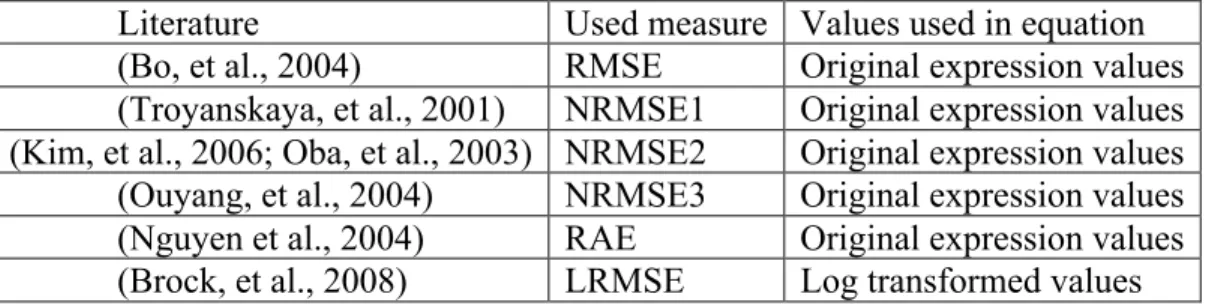
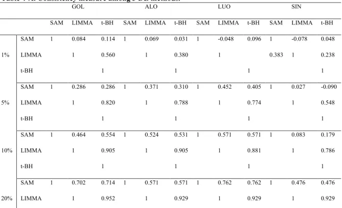
Table 4-A. Consistency measure among 3 DE methods... 53!
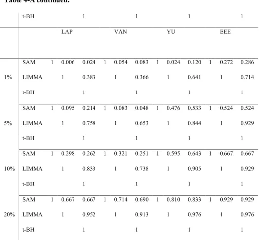
Table 4-B. Consistency measure among 4 classification methods.. ... 54!
Table 4-C. Consistency measure between 2 clustering methods... 56!
Table 5-A. Consistency measure between RMSEs and DE.. ... 59!
Table 5-B. Consistency measure between RMSEs and Classification.. ... 60!
Table 5-C. Consistency measure between RMSEs and Clustering.. ... 62!
Table 6-A. Linear Model between LRMSE and DE... 63!
Table 6-B. Linear model between LRMSE and Classification... 64!
&
-.,+&'(&/.012%,&
Figure 1.cDNA and Oligonucleotide microarray... 5!
ACKNOWLEDGEMENT
The work presented in this dissertation would have not been possible without the help of many people. I would like to express an eternal gratitude to several individuals who contributed their support and guidance to complete successfully. First of all, I would like to thank my advisor and committee chair, Dr.Tseng. During the PhD degree, I learned much statistical analyses and research methods about Biostatistics and Bioinformatics on working in his group and I am convinced that this knowledge will help me in the future. He always pushed me to achieve as much as I could, and taught me how to become a better biostatistician. He devoted his time to help me in navigating the dissertation. His ideas and tremendous support had a major influence on this dissertation. I would like to all committee members, Dr.Jeong, Dr.Lin, and Dr.Kong for providing their expertise, valuable advice, time and reviewing my dissertation during busy semester schedule. I would like to express thanks a bunch to Dr.Kong for sharing her valuable statistical advice, Dr.Jeong for mentoring me during the entire PhD degree, Dr.Lin for teaching me how to think creatively and logically on proposal and defense. I learned a great deal from all committee members. Thank you again.
To Dr.Sibille, I sincerely appreciate all support during PhD studies and his research field, which provided me to have had an invaluable opportunity analyzing depression and aging mouse and human data. It was a great training to play a crucial role as a stepping stone to the current
research. Thank you, Dr.Sibille. To Dr.Brock and Don Kang, I would like to thank for their assistance and valuable comments for this MV project.
I have heartfelt appreciation for all my friends, group lab members and Dr.Sibille’s lab members for being a good colleague on research and for always being beside me and offering their belief in me at times when I doubted myself.
I would like to especially thank my parents. None of this would have been possible without my loving parents and family. I share this accomplishment with them.
1.0 INTRODUCTION
1.1 THE BACKGROUND OF MICROARRAY EXPRESSION DATA
The microarray experiment is a new technology to investigate the expression levels of thousands of genes simultaneously. It has become one of the most indispensable tools that many biologists use to monitor genome wide expression levels of genes in a given organism. A microarray is typically a glass slide, which contains thousands of spots and each spot may contain a few million copies of identical DNA molecules that uniquely correspond to a gene. There are mainly two basic microarray technologies, cDNA array of dual-channel by Stanford group and high-density oligonucleotide arrays of one channel pioneered by Affymetrix. Each technology has its own merits and demerits. Figure 1 represents the schematic illustration of how microarrays experiments are performed for cDNA (a) and Oligonucleotide (GeneChip experiment) (b) microarrays. The main difference between two different platforms is how the genes are represented on the arrays, and the way that relative abundances of the transcripts are calculated. The cDNA microarray has two-color hybridization to be able to eliminate array to array noise and it is cheaper than Affymetrix. While cDNA produces relative abundant levels for target mRNAs corresponding to all probes on the array, the oligonucleotide array has only one sample, which hybridizes to a single array rather than target and reference sample and then returns an absolute mRNA level. In both platforms, the microarray gene expression data are represented as a G (gene) S (sample) matrix,
!
D
=
{
D
gs}
,where the entry is the mRNA expression level of gene g in experiment (sample) s.1.2 THE NEED OF MISSING VALUE IMPUTATIONS ON MICROARRAY EXPRESSION DATA
In the microarray experiment as mentioned in the previous subsection, missing values (MVs) frequently occur from various sources, such as dust, scratches on slide, insufficient resolution, or hybridization error, and etc. However, most statistical downstream analyses for microarray data such as DE (differentially expressed) gene detection, clustering and classification analyses require a complete data as the input. A naïve solution is simply to ignore and delete genes with missing values as a pre-processing step or replace missing entries with zero value, however, it may result in the loss of much critical information as it is known that microarray datasets have usually more than 5% missing values and up to 90% genes might be affected. To utilize the information of genes with missing values, missing entries can be substituted with estimated values using more robust imputation method. Even though numerous imputation methods have been introduced and are constantly developed during the past decade, no uniformly best method exists.(Bo, et al., 2004; Brock, et al., 2008; Kim, et al., 2006; Oba, et al., 2003; Troyanskaya, et al., 2001)The main reason is when using imputation methods for missing values that the performance of an imputation method strongly depends on the structure, nature and complexity of the data.
1.3 MV IMPUTATION METHODS AND PERFORMANCE MEASURES
Imputation methods have been usually evaluated by performance measures, such as RMSE. In such an evaluation, a complete data matrix with no missing value is used as a reference, a certain percentage of missing values are randomly generated and the missing values are imputed by a given MV imputation method. Variants of RMSE are used in the literature to quantify the differences of imputed
study of three imputation methods (KNN-impute, SVD-impute, Row-avg) for the estimation of missing values in gene microarray data with respect to the normalized RMSE by dividing it by average value over all observations in the true complete dataset. This measure is denoted here by NRMSE. (See method)He suggested KNN-Impute is a robust imputation method when comparing to Row-avg and SVD-impute. Even though KNN-Impute has been used as a popular imputation method due to its simplicity and fast computation so far, some recent papers have proposed further improved imputation methods. (Nguyen et al., 2004) suggested regression methods, which multiple imputations via ordinary least squares (OLS) and missing value prediction using partial least squares which accuracy for PLS imputation is higher for some ranges beyond moderate expression. From the results, they showed that KNN-impute is still more accurate, compared to PLS regression methods, when the true expression is near the mean, however outside of this range, PLS outperforms KNN-impute. (Oba, et al., 2003)suggested an imputation method based on Bayesian principal component analysis (BPCA). In the paper, estimation ability of BPCA is overall the best among KNN-impute, SVM-impute, and BPCA method. They used a normalized RMSE by dividing it by the standard deviation of the values corresponding to missing entries in the true complete dataset. We call it NRMSE2. (See method.) However, since BPCA assumes only a global covariance structure, the estimation with BPCA may not be accurate if genes have dominant local similarity structures and KNN-impute will be suitable in the case. (Ouyang, et al., 2004) proposed GMC-impute based on GMC (Gaussian Mixture Clustering) and model averaging. When using GMC-GMC-impute, the microarray data are assumed being generated by a Gaussian mixture of some number of components. GMC-impute shows better performance compared to naïve methods such as ZERO-impute, Row-avg, Col-avg, KNN-impute and SVM-impute in terms of normalized RMSE by dividing it by the root mean square of all the observations corresponding to missing entries in the true complete dataset in the study. We call it NRMSE3. (See method) (Bo, et al., 2004)introduced LSA-impute which is based on the least squares principle and utilizes correlations between both genes and arrays. The accuracy of LSA-impute is
normalized measure. (Kim, et al., 2006)suggested a local least squares imputation method (LLS-impute) to represent a target gene that has missing values as a linear combination of similar genes. The proposed LLS-impute method shows competitive results compared to KNN-impute and BPCA using NRMSE. This normalized RMSE is the same as (Oba, et al., 2003).
Novel methods for missing value imputation have been constantly developed during the last decade. Moreover, most of previous works on MV have been evaluated a MV method in terms of RMSE (Root Mean Squared Error), when comparing the new methods to the existing methods. Recently, a few papers have started to seriously take into account the influence of imputation methods on downstream analyses (de Brevern, et al., 2004; Jornsten, et al., 2005; Scheel, et al., 2005; Tuikkala, et al., 2006; Wang, et al., 2006). The results are, however, neither comprehensive nor conclusive. In other words, they employed the small number of datasets and methods. Additionally, a study is focused on a down-stream analysis. Even thougth a few people evoked an importance of biological impact on MV Imputation more recently, the take-home message still remained. Hence, in this dissertation, I will examine the biological impact assessments as well as classical RMSE-based measurements in comparison study of missing imputation methods to serve an insightful framework on MV imputation study. The detailed descriptions of MV methods and performance measures will be explained in the section 2.
1.4 MOTIVATION AND RESEARCH DESIGN OF OUR COMPARATIVE STUDY
Most evaluation of missing value imputation methods has been addressed by RMSE-based measures, instead of considering true biological impacts on down-stream analyses. Recently, a few people have issued this topic that the best imputation method detected by classical evaluation such as RMSE-based do not guarantee the smallest error to the impact of various statistical downstream analyses such as
Figure 1.cDNA and Oligonucleotide microarray.It represents how experiments are performed for cDNA (left) and Oligonucleotide (right) microarrays. In the top, it shows how microarrays are manufactured; and in the bottom, how RNA samples are obtained. In the middle, we can see images obtained after RNA samples hybridize to the microarrays. For cDNA microarrays (left), each dot represents a probe, and the red (or green) colors are proportional to the counts of RNA hybridized to that probe in the reference (or control) samples. Similarly, the intensity of white dots in Oligonucleotide arrays (right) represents the counts of RNA hybridized to that probe. Figure reproduced from (Simon, et al., 2004).
most common differentially expressed (DE) gene detection(Jornsten, et al., 2005).(Scheel, et al., 2005)examined the impact of imputation on the detection of DE (differentially expressed) genes using SAM and ANOVA. They proposed a novel imputation method, linear model based imputation (LinImp)
investigation covers false negative gene list as a biological impact measure. Specifically they counted the number of genes to be falsely declared as non-significant genes compared to gold-standard gene list, where gold standard gene list is defined by the significantly differentially expressed gene list in complete dataset. The focus has been only on differentially expressed gene detection in this paper. However, to draw a more general conclusion to effects of missing values on down-stream analyses, impacts to missing values in classification and other down-stream analyses as well as DE gene detection are needed to present. In clustering analysis, (de Brevern, et al., 2004) investigated the effects of missing value imputation on the stability of gene groups by hierarchical clustering using Conserved Pairs Proportion (CPP). However, in the paper, they presented KNN-imputation method is the most efficient replacement for missing value even though other further sophisticated imputation methods have been studied without ceasing. The limitation of this study is that they only carried out less powerful and inefficient imputation methods such as KNN-impute (KNN.e) and Zero-impute. In classification analysis and functional modules,(Wang, et al., 2006)demonstrated the effects of missing values imputation methods posterior to down-stream analyses. They compared the accuracy rates of three different classifiers, KNN, SVM, and CART classifier on down-stream analyses after imputing missing values using various imputation methods such as ZERO-impute, KNN-impute, LLS-impute, and BPCA in investigating which imputation tool is most robust. (Tuikkala, et al., 2006) investigated the impact of missing value imputation on K-means clustering and interpretation of GO terms from gene expression microarray data. Using 4 imputation methods including naïve method and BPCA, they explored how the agreement of estimated values for missing entries with the original data values and the original clustering results are returned by each imputation method. They employed ADBP (Average distance between partitions of genes) as a biological impact measure as well as normalized RMSE as a classical performance measure. 4 MV imputation methods including average methods and one clustering method are not sufficient to draw a conclusion in comparative study of MV methods.
More recently, (Brock, et al., 2008)showed a more comprehensive comparative study and proposed two selection schemes for selecting the best MV imputation method. Naïve and competitive imputation methods from the previous papers are utilized in this study. Under the assumption that the best MV imputation method depends on the structure and nature of input data, a series of data sets from various experimental designs (two-group comparison, multi-exposure and time series) are analyzed. A log-transformed version of RMSE (named LRMSE) is used as the performance evaluation measure. Through evaluation by LRMSE, they proposed two useful selection schemes of imputation methods, EBS (Entropy based selection) and STS (Simulation based self-training selection). In this comprehensive comparative study, they concluded that there is no universally best MV imputation method although three top methods such as LLS-impute, LSA-impute, and BPCA are very competitive and the accuracy on MV imputation depends on structure and nature of given data set. Even though the study tried to perform a large-scale comparative study, their focus is limited by RMSE-based evaluation. Thus, the previous works on MV imputation methods presents some partial conclusions using smaller number of data sets, comparing fewer MV methods, including fewer down-stream analysis methods in each category or applying inadequate evaluation indices. Hereby, the purpose of this dissertation is to provide a comprehensive comparative analysis to examine the biological impact of MV imputation in all three areas of down-stream analyses by addressing three major aims: (Aim 1A) To investigate whether applying different RMSE measures affects the performance ranking and decision of MV imputation method selection.; (Aim IB) To investigate whether applying different down-stream analysis methods in each category (i.e. SAM, LIMMA and t-test+BH for DE gene detection; LDA, KNN,SVM, and PAM for classification ;K-means, SOM for gene clustering) affects the performance ranking and decision of MV imputation method selection. (Aim 2) If selection of RMSE measure greatly affects the selection of MV imputation method in Aim 1A, investigate which RMSE measure is more consistent (correlated) with the biological impact measure. (Aim 3) Evaluate the consistency and correlation of the best RMSE measure
methods of column and row average method. These two methods are obviously of bad performance and are removed. Eight remaining MV imputation methods will keep being discussed in further sections. Eight MV imputation methods (1!m!M=8; KNN.e, KNN.c, SVD, OLS, PLS, LSA, LLS and BPCA) are considered, eight data sets (1!d!D1=8) for DE gene detection and classification and six data sets (1!d!D2=3) for gene clustering are evaluated, four missing value percentages (1!p!P=4; (r1, r2, r3,
r4)=(1%, 5%, 10% and 20%)) are considered and finally 100 independent simulations (1!n!N=100) are performed. In total, 8"11"4"100=35,200 times of random deletion from complete data matrix and then missing value imputation need to be performed. Due to the already high demand of computing, we skip the procedure of finding the optimal parameter for each MV imputation method in each data set and use the optimal parameters in the comparative study by Brock et al. (2008). For the optimal parameter in KNN and SVM classification, we fixed with the K=5 and linear kernel function, respectively after doing several simulation examinations, from k=1 to k=15 and 4 kernel functions using GOL, ALO, and LUO data set. To investigate quantitative and biological criteria for deciding which MV imputation methods perform better, three RMSE measures (NRMSE, LRMSE and RAE), three DE detection methods (SAM, LIMMA and t-test+BH), four classification methods (LDA, KNN, PAM, SVM) and two gene clustering methods (K-means and SOM) are considered. In gene clustering, the number of clusters is usually not known and usually difficult to estimate from the data. We perform k=5, 10 and 15 to select the best. Therefore, we have 8"11"4"100"3=105,600. RMSE evaluations, 8"8"4"100"3=76,800 DE gene detection evaluations, 8"8"4"100"4=102,400 classification evaluations and 8"3"4"100"2"3=57,600 for gene clustering evaluations. Throughout above proposed research design and 3 main Aims, we believe that the conclusions could provide an insightful conclusion for biological impact of MV imputation on down-stream analyses. To investigate the three Aims above, we apply Spearman’s rank correlation to quantify the consistency of selecting (ordering) MV imputation methods given any two criteria of either RMSE measures or biological impact measures. For example, figure 3 shows
BLCI. The exact consistency score from Spearman correlation is formulated below. For Aim 1A, we define,
where RMSEmdpni is the RMSE measure from MV imputation method m, data set d, MV percentage p, and simulation n and the RMSE measure i(i=1 meaning NRMSE, 2 for LRMSE and 3 for RAE). The measure corsp(!,!) is obtained by Spearman’s rank correlation. Intuitively, if
!
˜
r dpijRMSE"RMSE
=1, the two RMSE measures i and j give exactly the same rank order of the M=8 MV imputation methods and are considered consistent in MV imputation method selection.
Similarly, we define the consistency score for any two down-stream analysis measures in DE gene detection (BLCI), classification (YI) and clustering (ARI) for Aim 1B as
!
rdpnijBLCI"BLCI
=corsp
(
(BLCI1dpni,BLCI2dpni,...,BLCIMdpni),(BLCI1dpnj,BLCI2dpnj,...,BLCIMdpnj))
˜r dpijBLCI"BLCI
=median of rdpnijBLCI"BLCI
,1#n#N
{
}
,!
rdpnijYI"YI
=corsp
(
(YI1dpni,YI2dpni,...,YIMdpni),(YI1dpnj,YI2dpnj,...,YIMdpnj))
˜ r dpijYI"YI =median of rdpnijYI"YI,1 #n#N{
}
, ! rdpnij ARI"ARI=corsp
(
(ARI1dpni,ARI2dpni,...,ARIMdpni),(ARI1dpnj,ARI2dpnj,...,ARIMdpnj))
˜
r dpijARI"ARI
=median of rdpnijARI"ARI,1
#n#N
{
}
, , where ! BLCImdpni,, ! YImdpni, and !ARImdpni,are the BLCI, YI or ARI measures from MV imputation method m, data set d, MV percentage p, and simulation n and the different selections of down-stream analysis i (SAM, LIMMA, t-test+BH; LDA, KNN, PAM, SVM; K-means, SOM, hierarchical clustering).
!
rdpnijRMSE"BLCI
=corsp
(
(RMSE1dpni,RMSE2dpni,...,RMSEMdpni),(BLCI1dpnj,BLCI2dpnj,...,BLCIMdpnj))
˜ r dpij RMSE"BLCI =median of rdpnij RMSE"BLCI ,1#n#N{
}
, ! rdpnijRMSE"YI=corsp
(
(RMSE1dpni,RMSE2dpni,...,RMSEMdpni),(YI1dpnj,YI2dpnj,...,YIMdpnj))
˜r dpijRMSE"YI
=median of rdpnijRMSE"YI
,1#n #N
{
}
,!
rdpnijRMSE"ARI
=corsp
(
(RMSE1dpni,RMSE2dpni,...,RMSEMdpni),(ARI1dpnj,ARI2dpnj,...,ARIMdpnj))
˜ r dpijRMSE"ARI
=median of rdpnijRMSE"ARI
,1#n#N
{
}
,,where i is an index for RMSE measure and j for a down-stream analysis method.
In Aim 3, in addition to using the consistency measure for RMSE and biological impact measures for MV imputation method ranking, we further apply the following simple linear regression model to investigate the degree of correlation and the slope:
!
BLCImdpni="dpnij BLCI
+#dpnij BLCI
$RMSEmdpnj+%mdpnij
,where the linear model interprets how well RMSE measures can predict BLCI measures and !dpnij reflects the slope in data set d, MV proportion p, simulation n, RMSE measure i and DE
detection method j. We further define
! "dpij *(BLCI) = median of ˆ "dpij BLCI, 1 #n#N
{
}
and the 95% confidence interval ! ("dpij L;(BLCI) ,"dpijH;(BLCI))as the 2.5% and 97.5% quantile of the N slope estimate
!
ˆ " dpij
BLCI, 1
#n#N
{
}
. Intuitively, good missing value imputation results in low RMSE and high BLCI and we expect the ! estimates to be negative. When ! is negative and large in absolutevalue, differences of RMSE among different MV imputation methods contribute to real biological impact in BLCI and the method selection by RMSE is meaningful. If ! is negative but
close to zero, difference of RMSE does not affect the biological impact measure in BLCI and the selection by RMSE is redundant.
2.0 METHODS
2.1 DATA COLLECTION AND PREPROCESSING
For each data set that has MVs in the step to collect dataset, we deleted genes and samples with missing entries so that a complete data matrix without MVs can be used in the study. Thus, original size represents the size of matrix prior to pre-processing to delete missing values, whereas used size is matched by the matrix to be analyzed and evaluated in this comparative study. For clarity, Table 1 lists important features and characteristics of the data sets more details.
Table 1.The description of 11 datasets used in down-stream analyses.
DE/CL GOL 7129X72 1994X72 AML = 25 ALL = 47
Affy Min(expr)*=0 Max(expr)*=16.12 DE/CL ALO 6500X62 2000X62 Colon cancer = 40
Normal = 22
Affy Min(expr)*= 2.54 Max(expr)*=14.35
DE/CL LUO 6500X25 6433X25 PA*=16
BP*=9 cDNA Min(expr)*=0 Max(expr)*=9.6 DE/CL SIN 12600X102 1662X102 PT*=52 AP*=50 Affy Min(expr)*=1 Max(expr)*=14.10 DE/CL LAP 39009 X112 3098X71 PC*=62 M-PC*=9 cDNA Min(expr)*=-8.83 Max(expr)*=12.36 DE/CL VAN 25000X117 3196 X 97 BC*=51 BC-M*=46 cDNA Min(expr)*=0.87 Max(expr)*=1.20 DE/CL YU 37777X152 2532X89 Prostate cancer=66
Normal=23
Affy Min(expr)*=0 Max(expr)*=13.04 DE/CL BEE 7129X96 3577 X 96 OD*=10
AC*=86
Affy Min(expr)*=-3.32 Max(expr)*=17.01
Table 1 continued.
Gene clustering
SP.AFA 7681X18 4480X18 Time series,cyclic cDNA Min(expr)*=-2.71 Max(expr)*=4.76 Gene
clustering
SP.ELU 7681X14 5766X14 Time series, cyclic cDNA Min(expr)*=-6.22 Max(expr)*=4.95 Gene
clustering
CAU 4682X45 4616X45 Multi exposure Time series
cDNA Min(expr)*=3.00 Max(expr)*=11.44 DE: Differentially expressed gene detection, CL: Classification. PA*=Prostate adenocarcinoma, BP*= benign prostatic hyperplasiaz specimens, PT*=Prostate tumor samples, AP*=Adjacent Prostate, OD*= organ donors normal samples, AC*= adenocarcinoma, BC*=Breast Cancer, BC-M*=Breast Cancer with metastasis, PC*=Prostate Cancer, M-PC*= Metastasis Prostate Cancer in lymph node, Min(expr)*=minimum expression value after gene filtering and log transformation and Max(expr)*=maximum expression value after gene filtering and log transformation.
2.1.1 Datasets used in DE gene detection and classification
In differentially expressed (DE) gene detection analysis and classification, datasets are analyzed to search for differentially expressed genes in patients with two types or multi-class and to identify molecular biomarkers of disease classification and prediction to diverse tumor types. (Golub, et al., 1999) with two leukemia (ALL and AML), (Alon, et al., 1999) of colon tumor, and two prostate cancer datasets of (Yu, et al., 2004)and (Luo, et al., 2001) are analyzed. And four survival datasets are assessed to identify differentially expressed (DE) genes linked to survival outcome. One is (Singh, et al., 2002) including 102 prostate tissue samples, 52 tumor samples with 8 recurrent and 13 non-recurrent with survival time. Another is (Beer, et al., 2002) with 86 primary lung adenocarcinomas, including 67 stage I and 19 stage III tumors, and 10 non-neoplastic normal lung samples. And Stage I and III were also grouped into high-risk and low-risk subgroup, respectively. Another is prostate cancer dataset with relapse survival information by (Yu, et al., 2004). It contains including 23 organ donors normal samples and 66 tumors.
is composed of 97 primary breast cancers including 46 from patients who developed distant metastases within 5 years, 51 from patients who continued to be disease-free after a period of at least 5 years. For above four survival data sets with multi-class, we only select two sub groups from full samples in original data. We summarize the descriptions of original datasets and subgroups selected from original data sets used in DE gene detection and classification more details in Table 1 and following sections more details.
A. Golub (GOL) data
This Leukemia dataset (Golub, et al., 1999) is one of the most well known data set for methodological development. It contains 47 samples of acute lymphoblastic leukemia (ALL) and 25 samples of actue myeloid leukemia (AML) samples which are the combined training samples ( 38 samples: 27 ALL, 11 AML) as the primary samples and test samples (34 samples: 24 bone marrow and 10 peripheral blood samples) as the independent samples. The samples were assayed using Affymetrix Hgu6800 chips and data on the expression of 7129 human genes are collected initially. And then we deleted negative and zero gene expression values and then take log transformation. Finally, 1994 genes and 72 samples remained. The dataset has 0 and 16.1230 gene expression value as the minimum and maximum, respectively.
B. Alon (ALO) data
This dataset is originally collected in PNAS (1999) by (Alon, et al., 1999). The data matrix of Affymetrix oligonucleotide array contains about 6500 features and 62 samples. Some of the features display a hybridization signal that is many times stronger than their neighbors (~
the original paper. These outliers are deleted. To compensate of each EST on an array was normalized by dividing with the mean intensity of all ESTs on that array and multiplying with a nominal average intensity (50). The expression values of 2000 genes and 62 samples of 40 tumor and 22 normal colon tissues are finally remained. The dataset was downloaded on the web at http://www.molbio.princeton.edu/colondata.
C. Luo (LUO) data
The data were originally published in Cancer Research by (Luo, et al., 2001). The data included 16 prostate adenocarcinoma samples from Johns Hopkins Hospitals during October 1998 and March 2000, and 9 benign prostatic hyperplasia specimens from Johns Hopkins Hospital during February 1999 and November 2000. Total 25 samples and 6500 human genes were analyzed using cDNA microarray. We deleted some genes with zero and negative gene expression values, and took log2 transformation. Finally, 6433 genes and 25 samples remained.
D. Singh (SIN) data
The data set was originally published in Cancer Cell by (Singh, et al., 2002). The initial data set is composed of 12,600 genes and 102 samples including 52 prostate tumors and 50 non-tumor prostate samples using oligonucleotide microarrays. In the original dataset, it is already log2-transformed dataset. However, there exist too many zero values. After filtering out gene with zero values, 1662 genes remained for the further analysis in this study. In the original paper, this dataset indicated that 317 genes had up-regulated in the tumor samples and 139 genes had up-regulated in the normal samples. Additionally, this dataset has 21 patients with respect to
recurrence following surgery with 8 patients having relapsed and 13 patients having remained relapsed free for at least 4 years.
E. Lapointe (LAP) data
The prostate cancer dataset was originally published in PNAS by (Lapointe, et al., 2004). It contains 39009 genes and 112 samples with 62 prostate cancers, 41 normal samples, and 9 metastasis prostate cancer samples in lymph node. This original dataset has log2 transformation and some of missing values. After filtering out genes with missing values and additional filtering criterion, 3098 genes remained finally. Here the used specific criterion is to delete some more genes with low gene expression values such as mean < 1.5 and standard deviation < 1.2 for gene expression value in each gene.
F. van’tVeer (VAN) data
The data were collected in Nature 2002 by (van't Veer, et al., 2002). The data set is composed of 97 primary breast cancers including 46 from patients who developed distant metastases within 5 years, 51 from patients who continued to be disease-free after a period of at least 5 years. From the raw dataset, after eliminating gene with missing values and low expression values of less than log2 gene expression value 0.7,3176 genes are used for further analysis in this study.
23 organ donor normal samples and 37777 genes. All samples were analyzed using Affymetrix U95A microarray chips. In the original paper, they deleted some genes whose expression was very similar throughout all the samples to maximize the difference between the three groups (PC: prostate cancer, OD: donor prostate, AT: prostate tissues adjacent to cancer) and eliminated genes with low gene expression value less than the arbitrary cut-off value. And 19139 genes remained. After data preprocessing in which is filtered out genes with negative (or zero) gene expression value and missing values and log transformation are taken respectively. Finally, 2532 genes remained in the dataset for further analysis.
H. Beer (BEE) data
The data were originally published in Nature Medicine 2002 by (Beer, et al., 2002). The 86 lung adenocarcinoma samples were collected from the University of Michigan Hospital between May 1994 and July 2000 from 67 stage I and 19 stage III patients, and 10 non-neoplastic lung tissues were also obtained during that time. The total 96 samples were analyzed using Affymetrix HG6800 microarray chips. From the raw data set, after deleting negative and zero expression values and taking log transformation, 3577 genes remained in the dataset. In DE gene detection and classification, 86stage I and 10 non-neoplastic lung tissues are used.
2.1.2 Datasets used in Cluster analysis
In gene clustering, all data are pre-filtered (pre-processing) by a criterion to eliminate genes with negative and zero expression value.
A. Spellman-alpha (SP.AFA) data
This data set is originally collected to create a comprehensive catalog of yeast genes whose transcript levels varied periodically within the cell cycle by (Spellman, et al., 1998). DNA microarray samples from yeast cultures were synchronized by alpha factor arrest. It is a time series and cyclic data. After pre-processing, 4480 genes and 18 samples remained.
B. Spellman-elu (SP.ELU) data
This data set is also collected in(Spellman, et al., 1998). The only difference from Spellman-alpha data is the differently synchronized yeast by elutriation. After pre-processing, 5766 genes and 14 samples remained.
C. Causton (CAU) data
This data setis originally collected by (Causton, et al., 2001)to explore how gene expression in Saccharomyces cerevisiae is remodeled in response to various changes in extracellular environment, including changes in temperature, oxidation, nutrients, pH, and osmolarity. After pre-processing, 4616 genes and 45 samples remained.
2.2
MV METHODS DESCRIPTION
In microarray expression data, missing values frequently occur due to diverse sources, such as scratches, dust, insufficient resolution and hybridization error, etc on arrays. However,
expressed gene detection analysis, k-means clustering, and classification. One simple strategy is to delete genes with missing values and keep a complete matrix. However, this may lead to a loss of large useful information. Especially, it is rarely to have a set of complete values over all experiments. Therefore, in microarray experiment, more commonly suggestible strategy is to estimate missing values by borrowing the information of genes with similarity structure. During the last decade, although various imputation methods have been developed and proposed, as any given dataset, uniformly superior imputation is still ambiguous because each imputation method has own strength and weakness and imputing missing value largely depends on nature and structure of dataset. Some of imputation methods have a good performance on local structure, while others show better performance on global data structure. Therefore, in this comparative study, we employ 10 imputation methods including global and local imputation method.
2.2.1 Naïve methods
The most naïve way to impute missing values in microarray data is to insert the corresponding row/column averages or zero value. Such methods are highly inaccurate. In addition, (Troyanskaya, et al., 2001) already showed that row/column average method yields poor performance comparing to K-nearest neighborhood imputation method described below. We will omit the naïve methods in all analyses hereafter and focus on the more robust imputation methods.
2.2.2 K-nearest neighbor (KNN) based on distance/correlation
K-nearest neighbor introduced in (Troyanskaya, et al., 2001)finds the most similar k genes for the target gene with missing values based on euclidean distance (KNN.e) or pearson correlation measure (KNN.c). The method was among the first proposed methods and became popular due to its simplicity. The following steps show the algorithm for imputing the missing values in a given gene g,
Step1: Compute the Euclidean distance (or Pearson correlation) between g-th gene and all remaining genes using only those co-ordinates not missing in g-th gene. Select the most similar K genes.
Step2: Impute the missing entries of g-th gene by weighted averaging the corresponding coordinates of the K genes. The weights are chosen to be the inverse of distances or correlations.
Previous literatures suggested that although the result depends on K, the range of 10 to 20 provides good and the consistent imputation results. We will use K=10 in this thesis.
2.2.3 Singular Value Decomposition (SVD)
Singular Value Decomposition (SVD) introduced by (Troyanskaya, et al., 2001) approach first imputes all missing values using the row average imputation method in a preliminary step since SVD cannot handle the data matrix with missing values. It is then applied to create a set of mutually orthogonal principal components of expression patterns, so-called eigen-genes. SVD is then linear transformation of the expression data (A) from G genes S samples (arrays) to the reduced p S eigen-arrays, where p is the proportion of eigen-genes
which correspond to the largest eigen-values are selected values to reconstruct MVs in the expression matrix.
The singular value decomposition of A is A =
!
U
"
V
T (7)The columns of form the eigen-genes of , whose contribution to the expression in the eigen-space is quantified by corresponding eigen-values on the diagonal of matrix . The k most significant eigen-genes are selected to form the basis for the imputation process. The value of k is usually determined empirically. The missing entry is estimated from a linear combination of the k eigen-genes weighted by the regression coefficients. This process is iterated until the total change in the matrix A converges to a sufficiently small prefixed value. In previous literature, a range of 0.1~0.25 for p gives good and consistent results. We will use p=0.15 in this study.
2.2.4 OLS
Ordinary least squares imputation method introduced by (Nguyen et al., 2004) is based on local neighboring-based approach as KNN. While KNN is to impute a missing value by using a weighted average of K most similar genes, OLS is regressed over K most similar genes. Therefore, a missing value is imputed by the weighted average of predicted values of fitted regression of the gene with missing values onto each neighbor gene, where K most similar genes are selected by absolute Pearson correlation value and the weight is,
! w= r"x 2 1#r"x2 +10#6 $ % & & ' ( ) ) 2
, where is the correlation between the target gene (#) with MVs and the candidate gene (x). We will use K=10 in this study.
2.2.5 PLS
Repeated ordinary least squares a neighboring-based approach proposed by (Nguyen et al., 2004) and Bo et al. (2004) are to regress missing value over each of the k most similar neighbor genes as mentioned 2.3.3 part. Succinctly, missing values (MVs) are estimated through the weighted average of the predicted values from the regression of the target gene with missing values onto each neighbor gene. K-closest genes are selected by neighbor genes with largest absolute Pearson correlation value from the candidate gene set . Nguyen et al introduced a novel method Partial Least Squares (PLS). In this paper, they concluded that PLS has the strength to have uniformly better performance in view of accuracy across the wide range of observed gene expression, whereas KNN imputation method presents worse performance over some specific ranges of expression values.
The main difference of PLS (partial least squares) by Nguyen et al. (2004) from KNN is to use all the candidate gene expressions as well as the available values from the target gene to estimate missing values (MVs). More precisely, the procedure is like below,
Step1: PLS constructs a sequence of gene components with the candidate gene expression matrix and the available values of the target gene.
Step2: The target gene and candidate genes comprise missing values (MVs) and
available values, respectively. Denote the expression values of the target gene as ,
where and are available values and missing entries to be imputed of target gene g. And
the expression values of candidate genes for the target gene g are denoted by , where
is a
!
G
g"
S
gmatrix of available values corresponding to and comprises of available values corresponding to the MVs of target gene g, . Thus, PLS contains a training set ( , ) and the test set will be used to predict MVs ( ) of target gene g.Step3: Since the number of samples ( ) is much smaller than the number of available genes ( ) ( << ), dimension reduction is necessary. Thus, PLS imputation is a dimension reduction method,which extracts gene components sequentially to maximize the sample covariance between the target gene and the linear combination of the set of candidate genes. The more detailed procedure of dimension reduction is explained in the following steps,
Step4: The k-th PLS step seeks a weight vector,
!
wk(g) (Gg"1), such that
!
w
k(
g
)
=
argmax
w'w=1
cov
2(
Y
"Agw
,
y
gA)
, subject to the orthogonality constraintsw
k'(
g
)
Sw
d(
g
)
=
0
,"
d, 1
#
d
#
k
whereS
=
Y
"Ag'Y
"Ag. Thus, a sequence of weightw
1(
g
), ...,w
2(
g
)
are obtained from this step for each gene g with missing values (MVs). And according to the previous literature by (Brock, et al., 2008), the number of components isStep5: The PLS gene components of linear combinations with maximum covariance with target gene g,
!
t
kA(
g
)
=
Y
"Agw
k(
g
)
are computed. Therefore, PLS imputation captures the most important mode of covariance exhibited between the target gene and candidate genes first and the next most important mode is captured to be orthogonal to the first PLS components.Step6: Using the constructed PLS gene components as predictors, a linear regression model based on the available values is fitted. , where is a matrix of the KG PLS gene components and is the least squares regression coefficient estimates.
Step7: Next the test data is applied. That is, the expression values of candidate genes ( ), corresponding to missing entries of target gene ( ) are used to construct the test PLS components, based on only the training information (Step4 and Step5). That is, the test components are substituted into the training PLS regression model to predict the MV,
!
y
"g M=
T
*(
g
)
#
g " . 2.2.6 LSA-imputeLSA-impute introduced by (Bo, et al., 2004) is to estimate missing values based on least squares principle as utilizing correlations between both genes and arrays. They are called LSimpute_gene and LSimpute_array, respectively. The gene-based estimates are obtained by multiple OLS method using the K closest candidate genes, and the array-based estimates are attained by multiple-regression based on the arrays, where missing values in gene expression
absolute Pearson correlation values. Thus, LSA imputation is the combined method of gene-based and array-gene-based imputation estimates. In the paper, there are two variants of estimate combination. The first (LSimpute_combined) is to use a fixed global weighting of the estimates between LSimpute_gene and LSimpute-array. The best global weight of two estimates is determined by initially re-estimating from the known values in the gene expression matrix and minimizing the sum of errors for re-estimated data.
2.2.7 LLS-impute
LLS-impute proposed by (Kim, et al., 2006) is based on local least squares principle to represent a target gene with missing values as a linear combination of K coherent genes that have the large absolute Pearson correlation values from candidate gene set. As in OLS and LSA-impute, the LLS-impute is to estimate missing values by performing multiple regressing the candidate genes on target gene. However, the least squares estimates are determined by pseudo-inverse of K closest genes, where if the K closest genes have some missing values and its percentage is relatively small, then K neighboring genes are deleted in determining estimates, otherwise MVs are initially estimated by row-average imputation method.
2.2.8 BPCA
This approach is based on Bayesian principal component analysis (BPCA) proposed by (Oba, et al., 2003) to consist of three elements, (1) Principal component regression, (2) Bayesian estimation, (3) an expectation-maximization (EM)-like repetitive algorithm. It proceeds
the posterior distribution of the missing values. The posterior distribution of model parameters is iteratively estimated until convergence is reached. This approach is a time consuming method because no parameters have to be fixed as the algorithm itself sets up the appropriate PCA dimension. Moreover, since BPCA considers the global correlation structure of the data, this algorithm may not be well suited for data, which has a dominant local correlation structure.
2.3 DOWN-STREAM ANALYSES EVALUATED
To evaluate biological impacts of missing value imputation in down-stream analyses, we consider three types of analyses commonly seen in microarray; differentially expressed (DE) gene detection, classification and gene clustering. The specific methods evaluated are described below.
2.3.1 DE gene detection
A two-sample microarray experimental design aims at identifying differentially expressed (DE) genes between two different groups such as normal versus disease. Various statistical tests have been employed to identify DE genes. The two t-test statistics provides a simple statistical method for identifying DE genes. But t-test statistics is unstable when the sample size is small, which causes an increase in false discovery rate. Moreover, the other weakness has the problem of multiple testing. Thereby, we employ adjusted Benjamini-Hochberg (BH) t-test statistics and LIMMA method to cope with the problem of multiple testing and SAM method is used to handle small variance by adding a small positive constant to the
using three popular methods, Benjamini-Hochberg adjusted p-value from t-test, SAM, and LIMMA to identify differentially expressed genes. FDR is controlled at 5% and the default parameters are used in the packages.
2.3.1.1T-test + Benjamini-Hochberg (BH) adjusted p-value
Standard statistical method, t-statistics is applied here to compare treatment group versus normal group, or other conditions with two classes.
, where ! Sx1x2 =
#
(xi"x1) 2 +#
(xj "x2)2 n1+n2"2 (8)and are defined as the average levels of expression for g-th gene in class 1 and 2. represents the standard deviation of repeated expression measurements and and are the numbers of measurements in class 1 and 2. Since microarray experiments simultaneously monitor expression levels of thousands of genes, there is multiple comparison issue. To resolve the issue, many approaches have been introduced for adjusting multiple testing so far. Especially (Benjamini and Hochberg, 1995) adjusted p value is a popular step-up procedure which controls
the FDR (false discovery rate) defined as
!
E
false rejections
total rejections
"
#
$
%
&
'
, where if there are norejections in study, then it is defined by 0. Thus, if we control FDR at 0.05, then we can claim on average, no more than 5 % of the rejections are in error under some dependency structures with
p
rj
*
=
min
k=j...m{min(
m
Consider testing
!
H
1,
H
2,...,
H
mbased on the corresponding p-values,!
P
1,
P
2,...,
P
m , where each hypothesis is that there is no difference between class 1 and class2 for each gene.Step1: Let
!
P
(1)"
P
(2)"
...
"
P
(m)be the ordered p-values, and denote by the null hypothesis corresponding to .Step2: Step up. Compare to . If
!
p
(k )"
k
#
$
k
, then reject all of!
H
(1),
H
(2),...,
H
(k)and stop. Step3: Compare to . If!
p
(k"1)#
(
k
"
1)
$
%
k
, then reject all ofand stop.
Step4: Compare to . If
!
p
(k"2)#
(
k
"
2)
$
%
k
, then reject all of!
H
(1),
H
(2),...,
H
(k"2)and stop.Otherwise continue. Continue in this fashion until a stop or until no hypotheses are rejected.
Hence, adjusted p-values for Benjamini-Hochberg are shown below. It is a step-up method so we start from the opposite side.
=
= min( , )
= min( , )
=min( , )
And then we compare the adjusted p-values to $. All of the adjusted p-values that are less than $ correspond to rejections of null hypotheses using the given method.
T-test adjusted by BH procedure has the merit of fast computation and can be performed in excel without the need of programming. It, however, is usually less powerful and the t-statistic may be problematic when the variance component in the denominator is close to zero. SAM has been proposed to cope with unstable variance by adding a positive constant in denominator.
2.3.1.2SAM (Significance Analysis of Microarray)
Significance Analysis of Microarrays (SAM) by (Tusher, et al., 2001)computes a score to each gene on the basis of change in expression relative to the standard deviation of repeated measurements. SAM method adds a small positive constant to denominator of t-statistics as a fudge factor to avoid identifying falsely significant genes due to small variances. That is, if g-th gene has low expression values, variance in
!
tsam(g)can be high, due to small values of .
However, to compare
!
tsam(g)across all genes, the distribution of
!
tsam(g)should be independent of
the level of gene expression and of . Thus we choose a fudge factor, to make the coefficient of variation of
t
sam(
g
)
approximately constant as a function of by the similarapproach as Efron et al. In other words, constant is chosen to minimize the coefficient of variation.
!
t
sam(g)
=
x
1"
x
2s
x 1x21
n
1+
1
n
2+
s
0 , where = ! Sx1x2 1 n1 + 1 n2 = (xi "#
x1)2+#
(xj "x2)2 n1+n2"2 1 n1 + 1 n2 (9)SAM provides FDR (false discovery rate) to be calculated by Median (or 90th percentile) of # of falsely called genes by dividing # of genes called significant.
More precisely, the SAM algorithm is stated as
Step1: Order test statistics in equation 9 according to magnitude.
Step2: Based on null hypothesis that there is no difference between class 1 and class 2, Using permutation test, for each permutation, compute the ordered null (unaffected) scores.
Step3: Plot the ordered test statistic against the expected null scores.
Step4: Call each gene significant if the absolute value of the test statistic for that gene minus the mean test statistic for that gene is greater than a stated threshold.
2.3.1.3LIMMA
It is a tool for identifying differentially expressed genes involving comparisons between two groups proposed by (Smyth, 2004). The main idea is to fit a linear model to the expression data for each gene!!Empirical Bayes and other shrinkage methods are applied to borrow prior information across genes making the analyses stable even for experiments with small sample size. In the model, there are three main steps. The first step is to rearrange it in the structure of general linear models with arbitrary initial coefficients and contrasts of interest. The second step is to derive consistent and robust closed form estimators for hyper-parameters even for small sample size based on the marginal distributions of the observed statistics. The third step is to reformulate the posterior odds statistics in terms of moderated t-statistics in which posterior residual standard deviations are used in place of ordinary standard deviations. In the end, those steps make it possible to have more stable inference when even sample size is small as the approach proposed by Lonnstedt and Speed. This package then provides the B-H adjusted p value after multiple testing.
2.3.2 Classification
We performed classification with feature selection based on univariate t statistics using LDA, KNN (k=5), and SVM classifier with linear kernel function. Univariate method considers one variable (a feature) at a time, whereas multivariate method considers subsets of variables (features) together such as PAM. We adopted the simple univariate feature selection by t statistics. Weperformed leave one out cross validation (LOOCV), selected the top N=5, 10,
Youden Index(smallest error rate). For PAM, gene selection is embedded and we pick the threshold that generates the best accuracy.
2.3.2.1LDA classifier
In Linear Discriminant Analysis (LDA) proposed by (Fisher, 2000), each class is characterized by its vector of means or ‘centroid’. An unknown sample is evaluated by computing the scaled distance between its expression profile and each class centroid. The unknown is assigned to the class to which it is nearest. Thus, LDA can be thought of as a nearest centroid classifier. The procedure of LDA is described more precisely below.
We would like to classify unknown samples into one of K classes. To build a classifier, we obtain training samples per class, k=1,2,…,K, with g genes on each microarray. For each training sample, we observe class membership, sample information X and expression profile Y. For simplicity, we will utilize only two classes (1 or 2) in this study. Note that each expression profile is a vector of length m. We assume that expression profiles from class K are distributed as N ( ), the multivariate normal distribution with mean vector and covariance matrix . Call L ( ; ) the corresponding probability density function. Finally, we agree upon prior probabilities that an unknown sample comes from class k, k=1 and 2. Bayes’ theorem states that the probability that a sample comes from class k, given that sample’s expression profile, is proportional to the product of the class density and prior probability:
Pr(
Y
=
k
|
X
=
x
)
"
L
(
x
;
µ
k,
#
)
$
%
k (11) We call equation (11) the posterior probability that array x comes from sample k. LDA!
y
"=
argmax
k{
L
(
x
;
µ
k,
#
)
$
%
k}
(12)This can be shown to be the rule that minimizes misclassification error by Mardia et al. (1979).
The innards of the right side of equation (12) are proportional to
(13)
Since the covariance matrix % is the same for all classes, only the exponential component of equation (14) is relevant to classification. We can then rewrite equation (12) as
!
y
"=
argmax
k{
(
x
#
µ
k)
T$
#1(
x
#
µ
k)
#
2log(
%
k)
}
(14) Thus, a sample is assigned to the class to which it is nearest, as measured by the metric!
x
"
µ
2"
2log(
#
)
is the square of the Mahalanobis distance between x and &. We can further simplify the problem by assuming independence between genes. This allows us to simplify the LDA classification rule (14) to!
y
"=
argmax
kx
i *#
µ
ik$
i%
&
'
(
)
*
2 i=1 m+
#
2log(
,
k)
-.
/
0
/
1
2
/
3
/
(15) 2.3.2.2KNN classifierKNN classifier in (Belur V. Dasarathy., 1991) is based on a distance/similarity function for pairs of observations, such as the Euclidean distance. K nearest neighbors of a training data is
of optimal parameter selection to perform some tests using 3 CD (complete data set), GOL, ALO, and LUO with k=1 to k=15. Then the similarities of one sample from testing data to the k nearest neighbors are aggregated according to the class of the neighbors, and the testing sample is assigned to the most similar class. A major drawback of the similarity measure used in KNN is that it uses all features equally in computing similarities. It can lead to poor similarity measures and classification errors, when only a small subset of the features is useful for classification. Therefore, in KNN, confident feature selection is suggested.
2.3.2.3SVM classifier
SVM introduced in (Burges, 1998)provides a machine learning algorithm for classification Gene expression vectors can be thought of as points in an n-dimensional space. The SVM is then trained to discriminate between the data points for that pattern (positive points in the feature space) and other data points that do not show that pattern (negative points in the feature space). Specifically, SVM chooses the hyper-plane that provides maximum margin between the plane surface and the positive and negative points. The separating hyper-plane is optimal in the sense that it maximizes the distance from the closest data points, which are the support vectors. The mathematical background of SVM is like below, given a training set of
instance-label pairs , where
!
xi "Rnand
!
y"
{
1,#1}
l, thus, we consider the problem of separating the set of training vectors belonging to two separate classes. The support vector machines (SVM) require the solution of the following optimization problem:w,b,"
min
1
2
w
Tw
+
C
"
i lTraining vectors are projected into a higher dimensional space by the function . Here there are many possible linear classifiers that can separate the given data, but the only one to maximize the margin exists. In other words, SVM finds a linear separating hyper-plane to maximize the distance between it and the nearest data point of each class.
!
C>0is the penalty parameter of the error term. And then the various kernel functions such as linear, polynomial, radial basis function, sigmoid, and etc are applied with the equation (21). Each kernel function with the kernel parameters is explained in the following.
(21) 1) Linear:
!
K
(
x
i,
x
j)
=
x
iTx
j 2) Polynomial: ! K(xi,xj)=("
xiTxj +r)d, ! " >0.3) Radial basis function (RBF):
! K(xi,xj)=exp("# xi"xj 2), ! ">0. 4) Sigmoid: ! K(xi,xj)=tanh("xi T xj+r). 2.3.2.4PAM
The (Tibshirani, et al., 2002) uses the statistics
!
d
gk=
x
gk"
x
gw
k(
s
g+
s
0)
to selectgenes, where makes
!
w
k"
s
gequal to the standard error of the numerator, and is a fudge factor intended to guard against very large statistics for very small standard errors as like SAM method; by default, PAM chooses the median of the for . Without s , d is just a t-statistics comparing the mean of gene g in class k (1 or -1, e.g normal ordisease) with the overall mean of gene g. Hence, measures the difference between gene g in class k and gene g in all classes combined. A gene that discriminates one class from the rest will have a statistic of large absolute value. PAM then shrinks toward zero, eliminating the genes that do not provide sufficient discriminatory information. For a particular choice of shrinkage parameter ', the shrunken statistics is
!
d
~gk=
sign
(
d
gk)(
d
gk" #
)
+, where‘+’ means ‘positive part’ (22)Thus, all less than ' in absolute value are shrunken to zero, and the rest are shrunken to somewhere between zero and the