Vu, VT, Bui, TL and Nguyen, TT
A competitive co-evolutionary approach for the multi-objective evolutionary
algorithms
http://researchonline.ljmu.ac.uk/id/eprint/12539/
Article
LJMU has developed LJMU Research Online for users to access the research output of the University more effectively. Copyright © and Moral Rights for the papers on this site are retained by the individual authors and/or other copyright owners. Users may download and/or print one copy of any article(s) in LJMU Research Online to facilitate their private study or for non-commercial research. You may not engage in further distribution of the material or use it for any profit-making activities or any commercial gain.
The version presented here may differ from the published version or from the version of the record. Please see the repository URL above for details on accessing the published version and note that access may require a subscription.
For more information please contact [email protected]
http://researchonline.ljmu.ac.uk/
Citation (please note it is advisable to refer to the publisher’s version if you
intend to cite from this work)
Vu, VT, Bui, TL and Nguyen, TT (2020) A competitive co-evolutionary
approach for the multi-objective evolutionary algorithms. IEEE Access.
ISSN 2169-3536
Date of publication xxxx 00, 0000, date of current version xxxx 00, 0000. Digital Object Identifier 10.1109/ACCESS.2017.DOI
A competitive co-evolutionary approach
for the multi-objective evolutionary
algorithms
VAN TRUONG VU1, LAM THU BUI2, AND TRUNG THANH NGUYEN.3, 1
Le Quy Don Technical University, Ha Noi, Viet Nam (e-mail: [email protected]) 2
Le Quy Don Technical University, Ha Noi, Viet Nam (e-mail: [email protected]) 3
Liverpool John Moores University, Liverpool, UK (e-mail: [email protected]) Corresponding author: Trung Thanh NGUYEN (e-mail: [email protected]).
This work was supported in part by a grant no. NRCP1516-1-134, funded by the Newton Fund and managed by the Royal Academy of Engineering and the grant No. HNQT/SPDP/14.19, funded by Vietnam Ministry of Science and Technology
ABSTRACT In multi-objective evolutionary algorithms (MOEAs), convergence and diversity are two basic issues and keeping a balance between them plays a vital role. There are several studies that have attempted to address this problem, but this is still an open challenge. It is thus the purpose of this research to develop a dual-population competitive co-evolutionary approach to improving the balance between convergence and diversity. We utilize two populations to solve separate tasks. The first population uses Pareto-based ranking scheme to achieve better convergence, and the second one tries to guarantee population diversity via the use of a decomposition-based method. Next, by operating a competitive mechanism to combine the two populations, we create a new one with a view to having both characteristics (i.e. convergence and diversity). The proposed method’s performance is measured by the renowned benchmarks of multi-objective optimization problems (MOPs) using the hypervolume (HV) and the inverted generational distance (IGD) metrics. Experimental results show that the proposed method outperforms cutting-edge co-evolutionary algorithms with a robust performance.
INDEX TERMS Dual-population, Convergence, Diversity, Co-Evolution , Competitive.
I. INTRODUCTION
T
HERE exist many practical problems in which often-conflicted objectives need to be optimized simultane-ously; especially prolems in machine learning where we are seeking a model with the best performance in both accuracy and generalization measures. These problems are called multi-objective optimization problems (MOPs). Un-like single-objective optimization which can be easy to find the best single solution, in multi-objective optimization (MOO), a set of optimal solutions (called Pareto-optimal solutions) will be usually selected. Obviously, finding the largest number of Pareto-optimal solutions possible from the MOO is a vital but time-consuming task. Therefore, the MOO tries to find a set of solutions that satisfy both criteria: as close as possible to the Pareto-optimal front and as diverse as possible [1].Unlike single-solution-based algorithms, population-based algorithms like evolutionary algorithms (EAs) can find a number of solutions simultaneously and hence it has become
a major approach for dealing with MOPs [2]. Recently, Multi-objective Evolutionary Algorithms (MOEAs) have be-come one of the present trends in developing EAs. Various MOEAs like Pareto-based algorithms ( [3], [4]), indicator-based algorithms [5], decomposition-indicator-based algorithms [6], or direction-based algorithm [7] have been proposed. These MOEAs differ both in convergence as well as in diversity preservation. In general, these algorithms can be divided into three groups. The first one (i.e Pareto-based algorithms) allocates priority on handling the convergence and the second one (i.e decomposition algorithm) focuses on the diversity. Meanwhile, the last group (i.e indicator-based algorithms) considers both convergence and diversity by using an in-dicator like Hypervolume (HV). Typical inin-dicator-based al-gorithms are IBEA (Indicator-based evolutionary algorithm [5]); dynamic neighborhood MOEA based on HV indicator (DNMOEA/HI) [8]; a HV estimation algorithm (HypE) [9]; and S-metric selection evolutionary multiobjective optimisa-tion algorithms (SMS-EMOA) [10]. These algorithms have
an advantage that they do not require any additional diversity preservation mechanisms. However, when the number of objectives increases, the computational complexity of these algorithms also increases very quickly. This is their biggest weakness. This drawback has limited its application in solv-ing multi-and many-objective problems.
In general, using only a single algorithm to solve the problem of balancing between convergence and diversity in MOPs is not easy. Therefore, the current trend is to combine multiple algorithms. This approach can be divided into two main groups: Multi-algorithm approach [15] (i.e. using multiple algorithms on the same population) and multi-population approaches [16] (i.e. using multiple multi-populations, each corresponds to one objective ). In [15], to balance be-tween convergence and diversity, the researchers introduced a multi-algorithm based on Non-dominated Sorting Genetic Algorithm II (NSGA-II) and IBEA (named MABNI). To be specific, NSGA-II and IBEA ran on the same population. After a series of test trials, especially the ZDT and the DTLZ ones, the MABNI produced good results. In [16], instead of using the same population, the authors used multi-ple populations to cope with multimulti-ple objectives, in which each objective was optimized by one population. The au-thors adopted particle swarm optimization (PSO) for each swarm and designed a co-evolutionary multi-swarm PSO algorithm (named CMPSO). The experiment results showed that CMPSO is suitable for solving MOPs with two and three objectives.
The multi-population approach can be regarded as a co-evolutionary algorithm (CoEA). The general idea of CoEA is to break down a problem into a set of sub-problems and uses multiple populations to optimize different sub-problems. The CoEA can be categorized into two groups [17] which are competitive and cooperative ones. In the competitive approach, the fitness of each individual in one population is measured by the competition with some individuals in other populations. With regard to the latter group, a collaborative mechanism is used to determine the fitness of each individual. The first version of cooperative co-evolution was proposed in [18]. In [19] a framework of the CoEA was used for the flex-ible pickup and delivery problem with time windows. In this study, there are two separate populations; one is employed for diversification purpose while the other is used for evolu-tionary intensification. In [20] based on a cooperative CoEA with dual populations, a new hybrid learning algorithm was introduced to design a radial basis function neural network (RBFNN) models with feature selection. While the purpose of the first population is to find out the most significant input characteristics of RBFNN, the second one aims at discover-ing the optimal RBFNN structure. Shardiscover-ing the same idea, the authors in [21] employed a 2-population cooperative CoEA (named differential evolution-based coevolutionary multi-objective optimization algorithm (DECMO)). In DECMO, SPEA2 (Strength Pareto Evolutionary Algorithm 2) and DEMO (DE for Multiobjective Optimization)/GDE3 (Gener-alized Differential Evolution) models with a similar fitness
mechanism were used in the first and second population respectively. In general, the cooperative mechanism between multiple populations is favorably utilized by CoEAs to deal with MOPs. To interested readers, papers ( [16] and [22]) are good references for further understanding on this area of research. Unlike the cooperative CoEAs, there exists a lack of research addressing the competitive CoEAs ( [22]- [24]). In [23], the authors proposed a competitive and cooperative co-evolutionary model (named CCPSO) for designing multi-objective particle swarm optimization algorithm. In [24], a combination of competitive and cooperative mechanisms was proposed to solve MOPs in a dynamic environment.
Recently, there have been many studies addressing the problem of balancing convergence and diversity in solving more complex problems such as constrained multi-objective optimization problems (CMOPs) ( [25]- [27]), dynamic multi-objective optimization [28], many objectives ( [29]-[30]), or ensemble learning problems (with the objectives of maximizing accuracy and diversity of the ensemble). The main idea of these studies is mainly based on a combination of two Pareto-based and decomposition-based methods. In [25], the authors used a co-evolutionary algorithm using the two-archive strategy (called C-TAEA) for solving the CMOPs. In particular, C-TAEA utilized two populations, one named convergence-oriented archive (CA) and the other named diversity-oriented archive (DA). CA’s mission is to maintain convergence and feasibility. The DA, meanwhile, is responsible for preserving the convergence and diversity of the evolution process. The empirical results on benchmark and real-world problems showed the competitiveness of the proposed method in comparison with other state-of-the-art algorithms.
In [31], Ke Li et.al. dealt with convergence and diversity si-multaneously by employing a dual-cooperative co-evolution paradigm (DPP). With the first population, a Pareto-based mechanism was operated in order to maintain a solution set with satisfactory. The solutions of this population are randomly spread. Regarding the second population, diversity was preserved by the application of a decomposition-based mechanism. In order to guarantee this trait, solutions in this population are uniformly spread. Finally, a restricted mating selection mechanism (RMS) was employed to harmonize in-teractions between two co-evolving populations. In the RMS, two mating parents are chosen from both populations. Each of them is restrictively selected from its neighboring sub-regions with a large probability. Because of this selection, there is a possibility that the individual in the first population may not be found. If this happens, an alternative individual can be taken from the corresponding sub-region in the second population. In such a case, both mating parents are selected from the same population, rendering the co-evolutionary mechanism meaningless. To address these shortcoming, Vu et.al. [32] improved this model by proposing a new restricted selection mechanism as well as some small improvements in the DPP model to shorten the running time as well as achiev-ing better results. Ke Li et.al. [33] proposed a dual-population
approach for balancing convergence and diversity. The au-thors utilized a grid dominance relationship to maintain the convergence and a decomposition based selection principle to preserve well distributed solutions like the second population in the DPP.
Inspired by the co-evolution paradigm with encouraging results [31], we continue to explore in this direction. Specifi-cally, in our research, a competitive co-evolutionary approach is developed to solve multiobjective optimization problems. The difference between this paper and existing studies is detailed as follows. First, we utilize an other mating selection mechanism instead of the RMS mechanism to select two mating parents. Second, to generate two offsprings from the selected parents, we use a competitive model instead of the co-operative one.
In summary, our main contributions are summarized as follows:
(a) We present a new dual-population competitive evolutionary approach (DPPCP) that uses a competitive co-evolutionary mechanism instead of a co-operative one for interaction between two populations.
(b) We propose a new neighbor-based selection mechanism (NBSM) to select mating solutions instead of using restricted mating selection (RMS) mechanism like previous studies. (c) We perform extensive experiments on the proposed algorithm to compare and analyze results with existing and related algorithms.
The rest of this paper is organized as follows. In Sec-tion II, background algorithms are presented with two well-known algorithms (NSGA-II and MOEA/D) and the dual-population paradigm (DPP). Afterward, the detail of the proposed method is shown in Section III. Then, experimental results and discussions are given in Section IV. Finally, the paper is concluded in Section V.
II. BACKGROUND
A. NON-DOMINATED SORTING GENETIC ALGORITHM II (NSGA-II)
NSGA-II [3] is one of the most common algorithms among Pareto-based EMO algorithms. This is an improved version of NSGA [34]. In NSGA-II, based on the objective function values, each solution knows how many solutions it domi-nates and how many solutions that dominate it. Thereafter, a non-dominated sorting mechanism will be used to rank solutions and assign them to Pareto-fronts (F0,...,Fl,...,Fp).
All solutions on the same front will not dominate each other or be dominated by one another. Solutions on a front will dominate solutions on other fronts with higher ranks. Both populations of parents and offspring are joined in a hybrid population. Half of them are selected for the new population. To construct a new population, the selection will start from
F0 (i.e. the lowest rank front) to a front denoted as Fl.
Because all solutions onFlhave the same convergence, they
need a diversity mechanism to compare. NSGA-II used the crowding-distance as a secondary selection strategy. This
way, NSGA-II always tries to keep the convergence as much as possible.
In Pareto-based algorithms, convergence and diversity are considered in turn. In NSGA-II, for example, at each gen-eration, solutions are ranked using a non-dominated sorting method. As a result, a population is divided into multiple fronts. Individuals with lower ranks (i.e. corresponds to better convergence) are preselected. Then, solutions on the last front are selected up to the full size of a population by using a diversity selection approach (i.e. crowding distance). Therefore, in NSGA-II, the preservation of diversity is sec-ondary. It only guarantees diversity for a limited number of solutions in the population; the rest is selected mainly based on the convergence regardless of their diversity. This causes a limitation in solving problems with many-objective (i.e. more than three objectives) or difficult problems with the complicated Pareto-optimal set.
B. MULTIOBJECTIVE EVOLUTIONARY ALGORITHM BASED ON DECOMPOSITION (MOEA/D)
To balance convergence and diversity, a decomposition-based approach is also applied. In this approach, a complex MOP is decomposed into several problems and these sub-problems are solved in a collaborative manner [11]. A MOP may be divided into a group of single-objective problems (e.g. MOEA/D [6] and MOEA/D-DE (MOEA/D based on differential evolution) [12]) or a group of sub-MOPs without using any aggregation function (e.g. NSGA-III [13] and MOEA/D-M2M (a version of multiobjective optimization evolutionary algorithm-based decomposition) [11]). Because different solutions in the population are associated with dif-ferent sub-problems, diversity is naturally maintained [6]. Whereas, by optimizing sub-problems, the convergence crite-rion will be satisfied. However, the limitation of this approach is that algorithms may struggle to preserve diversity in high dimensional objective space. As discussed in [14] the reason comes from the contour lines of aggregation functions used in decomposition-based MOEAs.
MOEA/D [6] is a decomposition-based method. It de-composes MOPs into a set of single-objective optimization sub-problems through an aggregation method (such as the weighted sum, Tchebycheff and boundary intersection ap-proaches [35]). In order to address these sub-problems, a population-based algorithm is applied. In MOEA/D, each solution is associated with a sub-problem and the population consists of the best solution for each sub-problem. There-fore, the diversity among these sub-problems will result in the diversity in the population. In addition, a set of evenly spread weight vectors is used by MOEA/D to identify the search directions. Therefore, MOEAD can produce a uniform distribution of Pareto solutions.
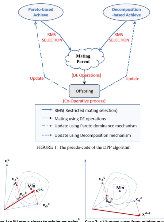
C. THE DUAL-POPULATION PARADIGM (DPP)
Given in Fig.1 is the general architecture of DPP model [31], which employed two co-evolving populations. The Pareto-based mechanism is used in the first population (named
Ap) and the decomposition-based mechanism is used in the
second population (namedAd). These populations engage in
a parallel evolution. At each generation, a restricted mating selection mechanism (RMS) allows them to interact with each other. In the RMS, the mating parent include three solu-tions, of which two are selected fromAd and the remaining
one is selected from Ap. Thanks to this, the parents could
give all the positive characteristics (i.e. the convergence and diversity) to the offspring. To update both Ap andAd, the
offspring utilizes the corresponding archiving mechanism. In the RMS process, there exist two cases. In the first case, if no solution is included in the selected sub-region in Ap,
an alternative solution will be chosen by the RMS in the corresponding one inAd. In the second case, if more than one
solution is found in the sub-region, only one solution will be selected.
This algorithm gives some promising results. However, there are two areas for possible improvements, as discussed below:
1. Restricted mating selection method:
The authors restrict the mating parents from neighboring sub-regions with a high probability (and there is only a low probability of these mating parents to be selected from the whole population). However, they only randomly select a neighboring sub-region fromAp regardless of whether this
sub-region contains any solutions in theApor not. This leads
to a high possibility that the selected sub-region does not contain any solutions (so an alternative solution has to be borrowed from the corresponding sub-region in Ad). This
may lead to an imbalance between the two populations.
2. The interaction between two co-evolving populations:
In DPP, the authors define the interaction as the way to generate offspring from mating parents. To be specific, they use differential evolution (DE) for offspring generation. This means they need three solutions (such as, xG
r1, xGr2, xGr3,
wherexG
r3 is the current solution,xGr1is a solution selected
from Ap andxGr2 is a solution selected fromAd) to create
new offspring (xGr3+1).
xGi+1=xGr3+F∗(xGr1−xGr2) (1) It is worth noting that in Eq.1,F∗(xGr1−xGr2)is a direction
vector. This vector is vital because it may help to direct the current vector to a new location that is closer to the global extremes or maybe even make it move further away from this position. Take Fig.[2] as an example. In case 1, using Eq.1, from the three parents xG
r1,xGr2,xGr3, we can obtain
an offspring solution xGi +1 whose position is closer to the global extreme position (denoted byMin) than its parents. On the contrary, in case 2, also using Eq.1, although the parents
xG
r1,xGr2,xGr3are close toMin, the offspring solutionx
G+1
i is
actually further away fromMinthan its parents. In DPP, the authors selectxG
r3andxGr1fromAdandxGr2fromApwith the
hope thatxGr1has good convergence properties andxGr2 has a promising diversity. In this way, we have a large chance to generate offspring having both of advantages. However, there still exist two major drawbacks:
(+) Choosing two out of three solutions from theAdand only
one fromApmay cause an imbalance in the co-evolutionary
process.
(+) Since the direction vector is made up of two solutions in two different populations, it could lead to unpromising out-comes, especially when the two populations are imbalanced (i.e. the convergence of a population is much better than the other). Let us consider a simple example in Fig.3. xG
r2 is
quite close to the Pareto front. Meanwhile,xGr1 is far from the Pareto front. Suppose that we are running with the Ad
population, by iterating over each region, for each sub-region (assuming the current sub-sub-region contains xGr3), we
make a random selection of two neighbour sub-regions (e.g. NB1, NB2). In these 2 sub-regions, NB1 contains a solution (e.g.xG
r2), while NB2 does not contain any solution. In this
case, NB2 will borrow a solution in the corresponding sub-region on theAp population(e.g. xGr1). After mating, based
on Eq.1,we might obtain the offspringxGi +1. It can be seen thatxGi+1has shifted to a position that is far from the Pareto-front. This leads to poorer results.
This paper attempts to address the aforementioned draw-backs. To do so, we propose a new dual-population co-evolutionary approach named DPPCP (The dual-population competitive co-evolutionary approach). This approach differs from the DPP model in two ways. First, it uses a competitive co-evolution rather than co-evolution to interact between two co-evolving populations. Second, it uses a neighbor-based selection mechanism (NBSM) instead of the RMS to select three different solutions on each distinct population.
These two models are explained in more detail in the next sections.
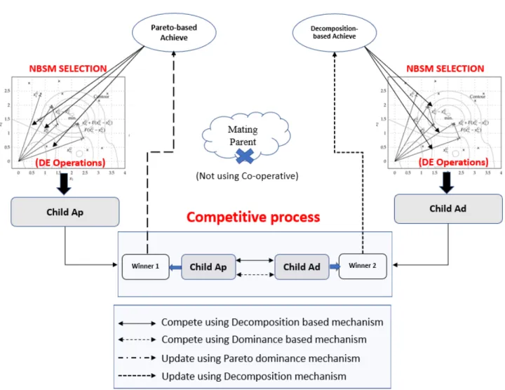
III. THE DUAL-POPULATION COMPETITIVE CO-EVOLUTIONARY APPROACH (DPPCP)
The general diagram of the DPPCP is given in Fig.4 and the pseudo-code of the proposed algorithm DPPCP is shown in Algorithm 1. There are two co-evolving populations: the first one (named Ap) is evolved by using the
Pareto-based mechanism; the other one (named Ad) utilizes the
decomposition-based mechanism to evolve. At each genera-tion, we use a neighbor-based selection mechanism (NBSM) to select three candidate solutions from each of the pop-ulations. After that, we use differential evolution (DE) to create two offspring named ChildAp (i.e. the offspring in
population Ap ) and ChildAd (the offspring in population
Ad). Next, we let ChildAd compete with ChildAp using
Pareto dominance-based metrics and choose the winner to updateAp. Similarly, we letChildApcompete withChildAd
using decomposition-based metrics and use the winner to updateAd. At the end of the co-evolution process, the final
population is a combination of bothApandAdpopulations.
The reason for this decision is that each of them uses a different optimal mechanism. While Ap uses true Pareto
front,Adutilizes idea point (a solution with the best objective
values known since running the algorithm) as the best goal to achieve. The roles of the two populations are the same.
FIGURE 1: The pseudo-code of the DPP algorithm
FIGURE 2: The way to generate offsprings from mating parents using DE operators
Therefore, in order to preserve the good properties of both populations (i.e. diversity and convergence), we decided to keep both populations in the final selected population.
As mentioned above, there are two differences between the DPPCP model and the DPP model: First, in the DPPCP, we do not use a co-operative co-evolutionary mechanism. In other words, we have eliminated the mating parents step to generate the offspring. Instead, we use a competitive mechanism to make two offspring interact with each other. Second, we use the NBSM mechanism to select three solu-tions in each population and use them to create two separate
offspring.
In general, the model is divided into four main steps: Initial-ization, NBSM selection, Competitive process, and Update population.
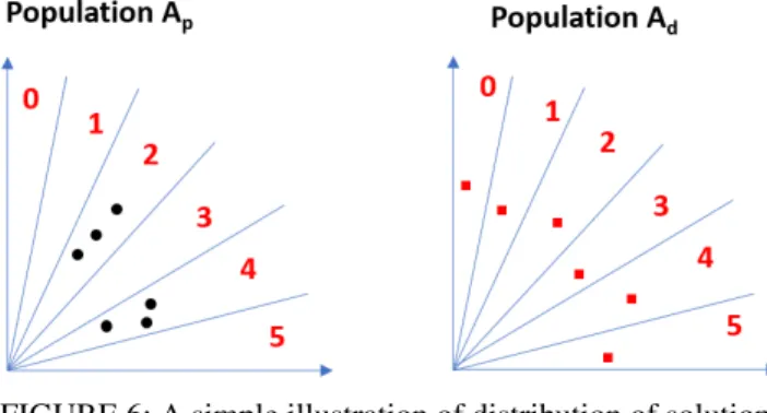
A. INITIALIZATION
At the first step, Ap and Ad (with the same size N) are
randomly generated. However, the distribution of individuals in the two populations is different. In Ad, N solutions are
assigned to different N sub-regions. To make sure that there is only one solution for each sub-region, the algorithm divides
FIGURE 3: A simple illustration of generating spring from mating parents
Algorithm 1:DPPCP Algorithm
input :M: The number of generations. T: The neighboring numbers N: The population size
output:Final PopulationApandAd
1 [Ap, Ad] =initializeP opulation()
2 W =InitializeU nif ormW eight() 3 B=InitializeN eighborhood() 4 Z∗=InitializeIdealP oint() 5 Znad=InitializeN adirP oint() 6 m←0 7 while m<Mdo 8 offspringAp←∅ 9 fori←1toN do 10 ChildAp, ChildAd= N BSM Selection(Ap, Ad, i, Bi) 11 W inner1 ==
CompeteDominate(ChildAp, ChildAd)
12 W inner2 ==
CompeteDecompostion(ChildAp, ChildAd)
13 UpdateAp(Winner1,Ap);
14 UpdateAd(Winner2,Ad);
15 UpdateZ∗andZnad
16 m++; 17 end 18 end
19 ReturnP←Ap∪Ad
the original region into N sub-regions (denoted as Si) by
using N uniformly distributed unit vectors denoted asλi(See
Fig.5). Eachλiwill be identified corresponding tosolutioni
(or each solution is assigned to only one sub-region). The algorithm utilizes the λ vectors to calculate the Euclidean distance between these vectors. Based on these distances, the
algorithm can determine which sub-regions are the neigh-bours of a solution. In the next step (i.e. evolutionary step), when a new solution is created, it is necessary to determine which sub-region it belongs to. This is done based on the calculation of the distance between the new solution and the
λ vectors. A sub-region will be selected if it contains the
λ vector which is closest to the new solution. However, it should be noted that, instead of including this new solution in this sub-region directly, a competition between the new solution and the existing solution in this sub-region will take place. The better solution (based on the fitness functions) will be selected to assign to this sub-region. By this way, there is exactly one solution in each sub-region andAdis distributed
evenly (i.e. diversity) in the objective space. UnlikeAd,Ap
does not rely on the even spread of N unit vectors. Therefore, N solutions in Ap are randomly assigned to N sub-regions
(Fig.6 gives an intuitive example of the distribution of solu-tions in each population. Ap does not contain any solution
in sub-regions 0, 1, 3, 5, while sub-regions 2 and 4 contain more than one solutions). This leads to a situation that a sub-region may either not have any solution or contain more than one solutions. Next, we find the T closest neighborhood sub-regions for each solution(by using the Euclidean distance). These neighborhoods play a vital role in the next steps.
B. THE NEIGHBOR-BASED SELECTION MECHANISM (NBSM)
In [6] the authors showed that: when solving continuous MOPs, in some mild conditions, neighborhood solutions should have similar structures. This means the neighborhood information is very important and it should be better if we use this important information in the orientation process for new solutions. For that reason, we prefer to choose mating parents from several neighboring sub-regions. As for the traditional DE operator [39],xGr1andxGr2(two components of the
FIGURE 4: System architecture of the dual-population competitive co-evolutionary approach
population. This random mating selection mechanism can ex-plore well. However, since there is no guidance information towards the Pareto set, it may lead to a degeneration problem. The RMS mechanism in [31] improved this weakness by using more information from neighboring sub-regions than from the whole population. However, as mentioned above, a drawback of the RMS mechanism is that the probability of selecting a sub-region inAp that contains at least a solution
is relatively low. At that time, the RMS borrows an alternate solution in theAd, which can lead to an imbalance between
two populations of the co-evolutionary process. This is the reason why we propose another selection mechanism (i.e. NBSM).
The pseudo-code of the NBSM mechanism is presented in Algorithm 2.
There are two underlying principles of the NBSM. Firstly, we want fairness in choosing the number of solutions to hybridize in the coevolutionary step. Secondly, the three chosen solutions used in the DE operator must be on the same population (in order to avoid the phenomenon as shown in Figure 3).
To generate new offspring (i.e. ChildAp or ChildAd),
we imitate the idea from MOEA/D-DE [12]. Specifically, in MOEA/D-DE, a solution y is generated from xr1 (i.e. the current solution),xr2andxr3according to Eq.2, and a new
solution is generated by a mutation operator onywith a small probability, according to Eq.3
yk= ( xrk1+F∗(xkr2−xrk3), with probability<CR xr1 k , with probability 1-CR (2) where CR and F are two control parameters
yk= ( yk+σk∗(uk−lk), with probabilitypm yk, with probability 1-pm (3) σk= ( (2∗rand)1η+1−1, ifrand <0.5 1−(2−2∗rand)η1+1, otherwise (4) Whererandis a uniform random number in [0,1];pmis the
mutation rate;ukandlkare the upper and lower bound of the
kthdecision variable, respectively.
Another major difference between the two RMS and NBSM mechanisms is the solution selection procedure in
Ap. For each small partition, we conduct a search across the
entire T neighborhood sub-regions instead of just choosing a random sub-region as in the RMS mechanism. This way, the
FIGURE 5: A simple illustration of initializing the population forAd
Algorithm 2:NBSMSelection(Ap,Ad,i,Bi)
input :Ap: the pareto-based population
Ad: the decomposition-based population
i: the current sub-region index
Bi: a set contains neighborhood indexes of
the current sub-region.
T: the neighborhood size; N: the population size
output:Q: Two mating parent
1 P1=M atSelectionAp()
2 P2=M atSelectionAd()
3 Solution1 =Ap[r1p]
4 Solution2 =Ap[r2p]
5 ifSubRegion(r1p)does not contain any solutions
then
6 Solution1 =Ad[r1p]
7 end
8 ifSubRegion(r2p)does not contain any solutions then
9 Solution2 =Ad[r2p] 10 end
11 ChildAp=DE(Solution1, Solution2, Ap[i]) 12 ChildAd=DE(Ad[r1d], Ad[r2d], Ad[i])
13 Return Q =(ChildAp, ChildAd)
probability of finding three solutions is much higher. In the case of any individuals cannot be found in the neighborhood sub-regions we borrow from theAd.
C. THE COMPETITIVE CO-EVOLUTIONARY MECHANISM (COMPETITIVE PROCESS)
In this step, two offspring solutionsChildAp andChildAd
in each population are selected to participate in tourna-ments. Fig.7 gives an intuitive explanation of this
mecha-FIGURE 6: A simple illustration of distribution of solutions in sub-regions
Algorithm 3:MatSelectionAd(Ad, i, Bi)
input :Ad: the decomposition-based population
i: the current sub-region index
Bi: a set contains neighborhood indexes of
the current sub-region.
T: the neighborhood size; N: the population size
θ: the neighborhood selection probability
output:[I,J]: Two sub-region indexes.
1 ifrand < θthen
2 Randomly select two indices I, J, fromBi
3 end 4 else
5 Randomly select two indices I, J from
{1,2, ..., N}
6 end
nism. Specifically, ChildAp competes against ChildAd
us-ing the Pareto-based rule (i.e. CompeteDominance method in Algorithm 1), a winner is selected to update Ap.
Algorithm 4:MatSelectionAp(Ap,i,Bi)
input :Ap: the pareto-based population
i: the current sub-region index
Bi: a set contains neighborhood indexes of
current sub-region.
T: the neighborhood size; N: the population size
θ: the neighborhood selection probability
output:[I,J]: Two sub-region indexes.
1 listN eighborAp←∅ 2 ifrand < θthen
// Select two sub-region indexes in Ap 3 fori←0toT do 4 forj←0toN do 5 ifAp[j]∈Bi[i]then 6 Add j tolistNeighborAp; 7 end 8 end 9 end
10 whilesize oflistN eighborAp <2do 11 Randomly select an index r from 1,2. . . .,N
12 Add r tolistNeighborAp
13 end
14 Randomly select two indices J and K from listNeighborAp.
15 end 16 else
17 Randomly select an index from{1,2, ..., N} 18 end
FIGURE 7: The competitive mechanism
the decomposition-based rule (i.e. CompeteDecomposition
method in Algorithm 1). We would like to highlight the ben-efits of competitive co-evolution by considering two possible cases:
(+) If two winning solutions belong to two different popu-lations. It means we have a solution which has good con-vergence and another with good diversity. This is what we expected.
(+) If two winning solutions belong to the same population (e.g.Ap). It means, one solution inAphas the convergence
better than its competitor (this is normal). Along with that, the remaining solution in Ap is more diverse than its
con-testant in Ad. It is interesting to note that, in this case, we
have one mating solution which has good convergence and the other which not only good convergence but also excellent diversity. Therefore, the offspring can get both of good traits. This is very different from the cooperative co-evolution in DPP.
D. UPDATE POPULATION
Algorithm 5:UpdateAp (winner1,Ap)
input : LimitedN um: The limited number of updated times
N: the Population size
output:Apafter updated
1 isN onDominte= False ;F lag= False; 2 fori←0toNdo
3 ifwinner1dominateAp[j]then
4 UpdateAp[j] by winner1; 5 Flag = True; 6 Num++; 7 ifNum==LimitedNumthen 8 Break; 9 end
10 else ifwinner1 andAp[j] are nondominated
then 11 isNonDominte = True; 12 end 13 ; 14 end 15 end
16 ifisNonDominte = True and Flag = Falsethen 17 Addwinner1toAp
18 Ap=crowdingDistanceSelection(Ap)
19 end 20 else
21 Randomly select an index from{1,2, ..., N} 22 end
The update mechanism in each population will be differ-ent. In research [31] the authors only updated Offspring to the nearest sub-region. This is to ensure the population diversity, but the probability that this solution will replace the sub-region is rather small (because it only compares to only one
sub-region, while there are some other sub-regions having much worse solutions). This may lead to the possibility that convergence will decrease. To improve this disadvantage, we used the updated idea of the MOEA/D algorithm for both populations. Specifically, we will iterate through all solutions in the neighborhood sub-regions in question and update them on a limited number of times (this helps to avoid having many similar solutions as well as speeding up the convergence of the population).
Specifically, the UpdateAd (winner2,Ad) method in
al-gorithm 1 is used in the same way as the MOEA/D-DE algorithm; whereas the UpdateAp (winner1,Ap) method is
shown in the algorithm 5.
It can be easy to see that, the way to updateApis different
from the one in the NSGA-II algorithm. We update Ap as
soon as the winner dominates a solution inApand
conduct-ingRankingandCrowdingDistanceSelectionmethods every time updating offspring. Meanwhile, the NSGA-II uses a list to store all of the offspring and performing ranking when the loop is finished.
It is highlighted that the new offspring requires being assigned to a certain sub-region. In this paper, to determine the suitable sub-region, the authors first measure the distance between its unit vector and the offspring’s objective vector. Which sub-region has the minimum distance will be selected to contain the offspring. It is also noted that the scaling of each objective function differs from each other. It means the value of objective functions can vary from low to high one. This leads to a situation that in the calculation of the Euclid distance, the low objective value is of no importance. Therefore, it is essential to standardize the objective func-tions in the same range of values. Here we perform the standardization [2] to the interval [0,1] as follows:
finorm= fi−Z ∗ i Znad i −Zi∗ (5) Where i ∈ {1,2, ..., m}; m is the number of objective functions.
The above analysis shows that basically Ap is similar to
NSGA-II; and Ad is similar to MOEA/D in terms of how
they work, but the details of the implementation are quite different. In the experimental results, we will further analyze these differences.
IV. EXPERIMENTAL STUDIES
In this step, we will perform experiments with the proposed algorithm to clarify some following problems. First, we compare the proposed method with some baseline algorithms (i.e. NSGA-II and MOEA/D-DE) and the state-of-the-art algorithms (ED/DPP in [31] and DPP2 in [32]). Via the comparison results, we could see how good the performance of the proposed method when comparing to the others. Next, we develop a variant namedDPPCP-Variant1and compare it to the DPPCP to know the effects of competitiveness. In order to know the effects of the NBSM mechanism, we create two variants namedDPPCP-Variant2andDPPCP-Variant3
and compare them to DPPCP. Finally, to know the interaction
between two co-evolving populations, we create two other variants named DPPCP-ApandDPPCP-Ad. After that, we conduct three test cases between NSGA-II andAp; MOEAD
andAd; andDPPCP-ApandDPPCP-Ad.
A. TEST PROBLEMS
In this paper, 32 test instances (ZDT1 to ZDT6, UF1 to UF10, WFG1 to WFG9 and DTLZ1 to DTLZ7) are used as benchmark problems. Among these, UF1 to UF7 [38] and WFG1 to WFG9 [36] and ZDT1, ZDT2, ZDT3, ZDT4, ZDT6 [40] are the bi-objective test problems; and UF8, to UF10 and DTLZ1 to DTLZ7 are tri-objective benchmarks. More detailed properties of DTLZ problems are summarized in Table 1.
TABLE 1: The DTLZ series test instances
Name Variablenumber Objectivenumber Geometry
DTLZ1 7 3 Linear DTLZ2 12 3 Concave DTLZ3 12 3 Concave DTLZ4 12 3 Concave DTLZ5 12 3 -DTLZ6 12 3 -DTLZ7 22 3 Disconnected B. PERFORMANCE METRICS
When measuring the performance of MOEAs, two common factors considered are convergence (the closeness between the obtained solutions set and the true Pareto optimal front) and diversity (the spread and distribution of solutions on the Pareto front). There exists a number of performance metrics to evaluate these factors such as generational distance (GD) [10], spacing metric (SP) [10], hypervolume (HV) [11] and inverted generational distance (IGD) [12], inverted genera-tional distance plus (IGD+) or stability [13]. Fig.8 shows the ability of each metric. The GD and SP metrics evaluate the convergence and uniformity respectively. Meanwhile, the IGD as well as the HV metrics measure are not only the convergence but also the diversity of a solution set.
In this paper, the IGD and HV are chosen as the main metrics. It is worth highlighting that the quality of a solution depends on the HV value. The greater the HV value is, the better the solution is. Besides, the lower the value of the IGD is, the better.
C. PARAMETERS SETTINGS OF MOEAS
Given in table 2 are the parameters of the NSGA-II and MOEA/D-DE. In each test trial, every algorithm is indepen-dently run 20 times. The population size (N) is set to 300 and the termination criterion of an algorithm is a predefined number of generation (M), which is constantly set to 300.000.
D. DPPCP AGAINST BASELINE ALGORITHMS
As mentioned above, the DPPCP uses two populations, one based on the Pareto mechanism (using the NSGA-II
FIGURE 8: Several performance metrics used in MOEAs TABLE 2: The parameter setting of the MOEAs
MOEAs Parameters settings
NSGA-II pc=0.9, pm=1/nvariables;µc= 20;µm= 20
MOEA/D-DE pm=1/nvariables,µm= 20, CR=1.0, F=0.5, σ= 0.9, T=20,0rand/1/bin0;nreplaced=2
algorithm), the other based on the decomposition mecha-nism (using MOEAD/DE algorithm). In order to assess the effectiveness of using the co-evolutionary mechanism, we compare the proposed algorithm with these two baseline algorithms (i.e. NSGA-II and MOEAD/DE). Table 3 and Table 4 provide the performance comparisons of DPPCP, MOEA/D-DE and NSGA-II on 32 test instances, with re-spect to the IGD and the HV metrics, rere-spectively. Based on experimental results, we can see that DPPCP achieves a better outcome than both NSGA-II and MOEA-D/DE. It wins in 26 out of 32 comparisons using the HV and the IGD metrics. It is worth noting that although NSGA-II is the worst among three candidates, it achieves the best IGD metric values on the UF4 and the UF5. Meanwhile, MOEA/D-DE obtains the best IGD metric values on the UF3, UF6, UF9, and WFG5. By contrast, DPPCP shows a poor result on the UF5 test instance. However, DPPCP shows better performance than the baseline algorithm on all the ZDT and DTLZ instances. These results indicate the effectiveness of DPPCP for achieving both convergence and diversity criteria.
E. DPPCP AGAINST STATE-OF-ART ALGORITHMS In [31], the authors compared the DPP algorithm with some state-of-the-art algorithms (e.g. MOEA/D-FRRMAB [41],
MOEA/D-RMS [42], MOEA/D-M2M [11], D2 MOPSO
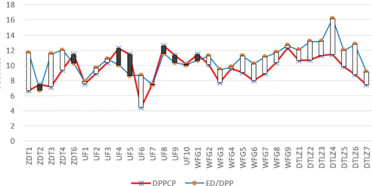
[43] and HyPE [9]) with competitive results. Therefore, DPP can be considered a state of the art algorithm. In this study, we focus on comparing the DPPCP with the original algorithm DPP (named ED/DPP) and the DPP2 algorithm [32], a modified version of this algorithm.
The results in Table 5 and Table 6 show that the proposed method (DPPCP) a is clearly better ED/DPP and DPP2 (it gives better metric value in 24 out of 32 comparisons). In ZDT instances, DPPCP give results better than ED/DPP in all instances, especially, in ZDT4 instance, DPPCP outper-forms ED/DPP about 10.000 times. In UF instances, ED/DPP
achieves better performance on UF5 and UF6 instances. However, DPPCP obtains better IGD metric values in other UF instances, even with UF1 it is better about 100 times. Similar to WFG instances, DPPCP achieves better metric values in all of the comparisons (except WFG5). These results show that the competitive co-evolution model pro-posed in this paper outperforms the co-operative co-evolution methods in ( [31], [32]).
F. EFFECTS OF COMPETITIVENESS
To verify the effect of the competitive co-evolutionary ap-proach, we have developed a variant (denoted as DPPCP-Variant1). In DPPCP-Variant1, there is no interaction be-tween the two populations, except for a connection in the selection stage (NBSM), where some individuals on theAd
side can be borrowed from theAp. Two offspringChildAp
andChildAdwill be used to update the population
immedi-ately instead of being used to compete in the DPPCP. The result is a combination of output from each population.
The performance comparisons are shown in Table 7 and Table 8 via the mean and standard deviation values. For each row in the table, we highlight the best value in bold.
In Table 7, we conduct the comparison between DPPCP and DPPCP-Variant1 using the HV metric. The DPPCP attains better metric values in all of the comparisons (except UF5, UF6, and UF9). Especially in Table 8, The DPPCP’s results are about ten times as good as DPP’s are with ZDT1, ZDT3, ZDT4, UF1, WFG3, WFG4, DTLZ5, DTLZ6 and about 100 times with WFG1, WFG2.
It can be seen that DPPCP shows better performance than
DPPCP-Variant1in most instances. Especially, DPPCP out-performsDPPCP-Variant1in the WFG series. Based on the results, it can be clear to see the advantage of the competitive co-evolutionary approach. It helps to achieve better results on both criteria (i.e. convergence and diversity).
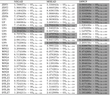
TABLE 3: Performance comparisons between the DPPCP with baseline algorithms using HV metric NSGAII MOEAD DPPCP ZDT1 6.647858e−015.3e−05 6.648386e−014.7e−05 6.655793e−010.0e+00 ZDT2 3.314961e−013.3e−05 3.315780e−015.1e−05 3.321892e−010.0e+00 ZDT3 5.168567e−011.2e−05 5.162200e−011.1e−05 5.170450e−010.0e+00 ZDT4 6.648548e−012.2e−05 6.649686e−019.8e−06 6.655913e−010.0e+00 ZDT6 4.031456e−011.4e−04 4.047282e−011.7e−08 4.053136e−010.0e+00 UF1 5.484432e−011.9e−02 6.636184e−011.3e−04 6.639659e−010.0e+00 UF 6.396909e−013.6e−03 6.572483e−012.8e−03 6.616692e−010.0e+00 UF3 4.571061e−013.4e−02 6.569119e−019.5e−03 5.965543e−010.0e+00 UF4 2.726602e−013.2e−04 2.458777e−015.8e−03 2.551797e−010.0e+00 UF5 2.374327e−012.8e−02 3.632481e−026.5e−02 8.999985e−020.0e+00 UF6 2.778372e−014.1e−02 2.024907e−017.9e−02 1.725421e−010.0e+00 UF7 4.195309e−016.1e−02 4.952861e−012.4e−03 4.954061e−010.0e+00 UF8 1.069511e−012.2e−02 3.295556e−012.3e−02 3.623309e−010.0e+00 UF9 4.296275e−011.2e−01 6.014756e−016.2e−02 5.565798e−010.0e+00 UF10 5.292133e−041.1e−03 5.944409e−022.7e−02 9.315613e−020.0e+00 WFG1 6.336915e−013.8e−04 6.347114e−012.2e−04 6.370891e−010.0e+00 WFG2 5.652985e−011.2e−05 5.646742e−011.3e−05 5.654082e−010.0e+00 WFG3 4.978645e−014.7e−05 4.980009e−016.1e−06 4.987931e−010.0e+00 WFG4 2.214379e−018.9e−05 2.212084e−011.1e−04 2.220795e−010.0e+00 WFG5 1.982352e−018.4e−05 1.988567e−012.2e−03 1.989817e−010.0e+00 WFG6 2.104230e−013.2e−03 2.128723e−014.5e−06 2.136358e−010.0e+00 WFG7 2.129812e−014.4e−05 2.128570e−018.1e−06 2.136157e−010.0e+00 WFG8 1.676837e−012.3e−02 1.704603e−012.4e−02 2.114787e−010.0e+00 WFG9 2.433160e−015.0e−04 2.438831e−015.5e−05 2.449073e−010.0e+00 DTLZ1 7.952908e−012.2e−03 7.849171e−012.9e−04 8.027772e−010.0e+00 DTLZ2 4.145143e−012.7e−03 4.185581e−018.5e−04 4.294453e−010.0e+00 DTLZ3 4.237451e−012.2e−03 4.192297e−019.9e−04 4.298513e−010.0e+00 DTLZ4 4.135101e−011.9e−03 4.121623e−012.2e−02 4.245304e−010.0e+00 DTLZ5 9.540642e−023.0e−05 9.469685e−027.7e−06 9.579286e−020.0e+00 DTLZ6 6.407350e−021.0e−02 9.566239e−027.8e−07 9.678412e−020.0e+00 DTLZ7 3.120551e−011.2e−03 2.770128e−011.6e−02 3.103702e−010.0e+00
G. EFFECTS OF THE NBSM MECHANISM
To further understand the effects of the NBSM mechanism, we extend this mechanism to two other variants as follows:
1. DPPCP-Variant2: This variant is different from DPPCP in that it chooses two sub-regions in the Ap. If the
sub-regions do not contain any solution, it randomly selects from the Ap instead of borrowing from theAd such as DPPCP.
This experiment aims to show the importance of selecting solutions in the neighborhood sub-regions.
2. DPPCP-Variant3: In Ap, instead of carefully selecting
two mating parents from all neighborhoods of the current sub-region, this variant randomly selects two neighborhood sub-regions regardless of whether they contain any solution or not. If two sub-regions do not contain any solution, they borrow from two sub-regions in the Ad respectively.
This experiment aims to show the importance of searching for neighborhood solutions in the whole neighborhood sub-regions.
The performance comparisons between DPPCP with two variants, regarding the IGD and the SPREAD metrics, are presented in Table 9 and Table 10. It is clear that DPPCP is the best candidate: it obtains better metric values in 20 out of 32 comparisons. On the contrary, DPPCP-Variant2 is the worst among them with IGD metric. Meanwhile, DPPCP-Variant3 obtains the poor spread.
In short, our proposed NBSM mechanism, which fully utilizes the guidance information of the neighborhood, is effective.
H. INTERACTION BETWEEN TWO CO-EVOLVING POPULATIONS
In this section, we clarify the effect of using dual populations. Specifically, we consider two main points:
1. The effect of using competitive co-evolution on each population.
2. The effect of the interaction between two populations. Specifically, we first compareApwith the NSGA-II
algo-rithm andAdwith the MOEA/D-DE algorithm. As discussed
above, the algorithms used inApandAddiffer from baseline
algorithms (i.e. NSGA-II and MOEA/D) at three main points: (a) the mating parent selection mechanism (i.e. NBSM); (b) the way to generate offspring (i.e. competitive method); and (c) how to update Offspring to populations. Through this experiment, we will know whether co-evolution helps individual populations to evolve better than independent evo-lution.
To implement this comparison, we create two new variants of the DPPCP algorithm:DPPCP-AdandDPPCP-Ap. These variants are very similar to the DPPCP algorithm, except that at the last step they only get the results done by theAp (for
DPPCP-Ap) and by theAd(forDPPCP-Ad).
The performance of NSGA-II and DPPCP-Ap are pre-sented in Table 11, Table 12; and Table 13, Table 14 show the results of comparisons between MOEA/D-DE and DPPCP-Ad. It is clear that DPPCP-Ap and DPPCP-Ad give bet-ter results than NSGA-II and MOEA/D-DE respectively.
DPPCP-Ap wins in 25 out of 31 comparisons,DPPCP-Ad
obtains better in 22 out of 31 comparisons using the IGD metric. Through experimental results, we realize that the effectiveness of baseline algorithms is enhanced by utilizing
TABLE 4: Performance comparisons between the DPPCP with baseline algorithms using IGD metric NSGAII MOEAD DPPCP ZDT1 5.788071e−054.8e−06 5.556843e−053.3e−07 3.093510e−050.0e+00 ZDT2 5.968199e−052.9e−06 4.660528e−054.7e−08 3.241247e−050.0e+00 ZDT3 4.146423e−051.9e−06 8.838159e−057.9e−07 2.623904e−050.0e+00 ZDT4 5.699439e−052.2e−06 5.906846e−055.0e−07 3.104248e−050.0e+00 ZDT6 7.378607e−054.2e−06 4.628025e−056.2e−09 3.135962e−050.0e+00 UF1 3.546947e−036.0e−04 6.903693e−055.0e−06 5.686509e−050.0e+00 UF 1.066904e−032.9e−04 3.608501e−042.4e−04 1.700001e−040.0e+00 UF3 7.154636e−031.8e−03 1.702418e−041.5e−04 1.820430e−030.0e+00 UF4 1.358224e−032.4e−05 1.940253e−032.3e−04 1.676999e−030.0e+00 UF5 4.394656e−028.3e−03 6.607502e−021.7e−02 1.547979e−010.0e+00 UF6 8.797878e−033.8e−03 3.479782e−038.8e−03 2.268674e−020.0e+00 UF7 1.859278e−031.7e−03 1.085036e−042.4e−05 1.185823e−040.0e+00 UF8 2.981191e−031.7e−04 9.841127e−044.3e−04 8.438084e−040.0e+00 UF9 2.732983e−032.0e−03 2.165702e−031.5e−03 2.269156e−030.0e+00 UF10 5.161469e−033.7e−03 4.986122e−036.2e−04 4.938679e−030.0e+00 WFG1 3.200666e−042.3e−05 2.702204e−042.7e−05 7.811839e−050.0e+00 WFG2 1.174109e−041.1e−05 6.057198e−046.6e−06 8.474260e−050.0e+00 WFG3 6.512669e−053.3e−06 5.476262e−059.3e−08 3.343249e−050.0e+00 WFG4 5.717426e−052.8e−06 6.238275e−051.3e−06 3.390037e−050.0e+00 WFG5 9.330129e−045.7e−07 9.337936e−043.8e−07 9.303355e−040.0e+00 WFG6 1.122812e−046.5e−05 9.139109e−051.4e−07 5.394634e−050.0e+00 WFG7 3.877603e−051.7e−06 4.054086e−051.9e−08 2.255773e−050.0e+00 WFG8 2.747423e−032.2e−03 3.174261e−032.4e−03 8.095268e−040.0e+00 WFG9 4.337451e−055.0e−06 4.071753e−051.1e−07 2.269694e−050.0e+00 DTLZ1 3.201110e−041.9e−05 3.474762e−041.3e−06 2.526425e−040.0e+00 DTLZ2 4.355620e−042.4e−05 4.306742e−043.0e−06 3.343429e−040.0e+00 DTLZ3 6.953162e−042.1e−05 7.211632e−046.2e−06 5.305681e−040.0e+00 DTLZ4 7.724318e−041.2e−04 7.911537e−041.3e−04 5.417136e−040.0e+00 DTLZ5 6.185971e−064.8e−07 1.516055e−051.1e−07 3.674228e−060.0e+00 DTLZ6 3.789467e−042.9e−04 3.453845e−053.1e−08 8.785615e−060.0e+00 DTLZ7 1.204211e−036.4e−05 2.612999e−031.7e−04 1.181486e−030.0e+00
a competitive co-evolutionary approach.
We continue comparing the results of each independent population (i.e. Ap andAd) using co-evolutionary
mecha-nisms with the result of combining both dual populations. By this comparison, we would like to examine whether or not the use of dual populations combines the quintessence of both populations.
Table 15 and Table 16 shows the results of comparisons between DPPCP,DPPCP-Ap, andDPPCP-Ad. It is clear that DPPCP achieves better values in most instances. This shows that thanks to the co-evolution mechanism, with interactions between solutions in two populations that the final population can get the advantages from both populations. It can be said that this population is likely to be able to balance both convergence and diversity.
The final solutions obtained by the DPPCP algorithm and the true PF on the DTLZ, UF, WFG and ZDT series are plotted in Fig.12-15. From these figures, we find that the proposed algorithm can find the approximation set that covers entirely the true PF.
I. CPU TIME COMPARISON
To compare the runtime of the algorithms, we analysed the CPU time cost of the proposed algorithm (DPPCP) with two baselines (NSGA-II and MOEA/D) and the co-evolution algorithms ED/DPP algorithm. We conducted comparisons on 31 problems. To get the most accurate assessment, all algorithms are implemented injMetal5(an integrated JAVA framework). It can be downloaded from http://jmetal.github. io/jMetal/. We run multithreading with 8 cores on computers configured as Intel Xeon E5-2620, 16gb Ram. Experimental
results are shown in Fig.9-11. We experimented with two different generation parameters which are 3000 (Fig.9-10) and 300,000 (Fig.11).
Suppose that M is the objective number; N is the pop-ulation size and T is the neighbour size. The time com-plexity of MOEA/D in one generation (iteration) is only
O(NTM), where M, TN. Meanwhile, O(M N2) is the
time complexity of NSGA-II algorithm. The DPPCP and ED/DPP algorithms maintain two coevolving populations. The main running steps of these two algorithms are similar to the MOEA/D algorithm. Thus, the complexity in these main steps is still O(NTM). However, small steps in the algorithms often have to be processed twice for two popu-lations so the calculation time will take more than baseline algorithms. Results with CPU time show this clearly. As you can see in Fig.9, the MOEA/D algorithm costs the least CPU time, followed by the NSGA-II algorithm. These two baseline algorithms take less time than the two DPPCP and ED/DPP algorithms. Fig.10 shows the comparison of the two co-evolution algorithms. The white boxes indicate that the DPPCP algorithm runs faster and vice versa with the black boxes. It is evident that with a loop count of 3000, the DPPCP algorithm runs faster than ED/DPP in most test cases. The result is similar for these two algorithms when the number of iterations increases to 300,000, as shown in Fig.11. The explanation for this result may be in the step of updating the child solution into the Ad population. While DPPCP updates with a limited number (K<T) of neighbourhood solutions (the time complexity is O(K)), in ED/DPP the author proceeds through all sub-regions to calculate distances and find the nearest sub-region and compare the child solution with
so-FIGURE 9: CPU time comparisons between for algorithms on different test instances (with the number of generations is 3000)
FIGURE 10: CPU time comparisons between for algorithms on different test instances (with the number of generations is 3000)
TABLE 5: Performance comparisons between the DPPCP with state-of-art algorithms using HV metric ED/DPP DPP2 DPPCP ZDT1 6.503543e−011.9e−02 6.648341e−014.6e−05 6.655793e−010.0e+00 ZDT2 3.062317e−017.8e−02 3.315689e−013.8e−05 3.321892e−010.0e+00 ZDT3 5.137847e−012.3e−03 5.162233e−019.3e−06 5.170450e−010.0e+00 ZDT4 0.000000e+ 000.0e+00 6.649716e−011.0e−05 6.655913e−010.0e+00 ZDT6 4.052969e−011.9e−05 4.047282e−015.4e−08 4.053136e−010.0e+00 UF1 6.095147e−011.5e−02 6.635853e−011.4e−04 6.639659e−010.0e+00 UF 6.071246e−019.4e−03 6.568236e−011.6e−03 6.616692e−010.0e+00 UF3 4.299732e−015.4e−02 6.521115e−011.5e−02 5.965543e−010.0e+00 UF4 2.384583e−017.3e−03 2.438856e−014.2e−03 2.551797e−010.0e+00 UF5 1.642984e−036.7e−03 1.208023e−019.1e−02 8.999985e−020.0e+00 UF6 9.514643e−025.0e−02 2.001687e−018.5e−02 1.725421e−010.0e+00 UF7 4.701857e−018.9e−03 4.958239e−018.2e−04 4.954061e−010.0e+00 UF8 2.564091e−013.3e−02 3.271188e−011.6e−02 3.623309e−010.0e+00 UF9 5.107049e−013.8e−02 5.646465e−013.1e−02 5.565798e−010.0e+00 UF10 0.000000e+ 000.0e+00 7.045457e−021.4e−02 9.315613e−020.0e+00 WFG1 4.500378e−016.6e−02 6.347178e−013.6e−04 6.370891e−010.0e+00 WFG2 5.635474e−017.7e−04 5.646761e−011.2e−05 5.654082e−010.0e+00 WFG3 4.922166e−012.6e−03 4.979994e−014.2e−06 4.987931e−010.0e+00 WFG4 2.117675e−011.3e−03 2.211018e−011.4e−04 2.220795e−010.0e+00 WFG5 1.995414e−012.1e−03 1.987193e−012.8e−03 1.989817e−010.0e+00 WFG6 2.109626e−011.5e−03 2.128725e−013.8e−06 2.136358e−010.0e+00 WFG7 2.129709e−011.8e−04 2.128533e−016.8e−06 2.136157e−010.0e+00 WFG8 1.576003e−011.8e−02 1.732010e−012.6e−02 2.114787e−010.0e+00 WFG9 2.412725e−011.6e−04 2.438372e−014.6e−05 2.449073e−010.0e+00 DTLZ1 3.981344e−021.6e−01 7.848863e−011.7e−04 8.027772e−010.0e+00 DTLZ2 4.325969e−011.5e−03 4.185189e−019.8e−04 4.294453e−010.0e+00 DTLZ3 8.816880e−021.7e−01 4.182285e−011.1e−03 4.298513e−010.0e+00 DTLZ4 4.198804e−011.5e−03 4.065588e−013.0e−02 4.245304e−010.0e+00 DTLZ5 8.724304e−022.3e−03 9.469878e−029.7e−06 9.579286e−020.0e+00 DTLZ6 9.656330e−021.2e−05 9.566300e−028.0e−07 9.678412e−020.0e+00 DTLZ7 3.129314e−012.5e−03 2.800935e−016.8e−03 3.103702e−010.0e+00
lution in this sub-region to update (the time complexity is
O(NM)). This is the main reason leading to the difference in CPU time between these two algorithms.
V. CONCLUSION
In this paper, we presented a competitive co-evolutionary approach (DPPCP) for balancing between convergence and diversity in MOEAs. Specifically, we use dual-population competitive co-evolutionary approach with a pair of popu-lations evolved in parallel. One uses the Pareto-based mecha-nism to obtain a better convergence and the other one uses the decomposition-based technique to maintain the diver-sity. These populations interact with each other via a new neighborhood based selection mechanism (NBSMS) and a competitive mechanism. We have evaluated the proposed model on four sets of benchmark problems. The performance of the DPPCP is compared with the baseline algorithms, the original version DPP and some variants using the HV and IGD metrics. The empirical outcomes show that the DPPCP model is better on test instances. By comparing DPPCP with baseline algorithms, the empirical results pointed out the efficacy of the new competitive co-evolutionary approach in balancing diversity and convergence in solving MOPs. This is our first study of applying competitive co-evolution to multi-objective optimization problems. The proposed method can still be improved and expanded in several aspects such as how to choose a final population that not only ensures diversity but also approximates the Pareto optimal solution set. Besides, in an extension of this work, we also plan to apply the approach to finding optimal parameters as well as features for machine learning models.
REFERENCES
[1] Lam Thu BUI, ed. Multi-Objective Optimization in Computational Intelli-gence: Theory and Practice: Theory and Practice. IGI global, 2008. [2] Deb, Kalyanmoy. Multi-Objective Optimization Using Evolutionary
Algo-rithms. Vol. 16. John Wiley and Sons, 2001.
[3] Deb, Kalyanmoy, et al. "A fast and elitist multiobjective genetic algorithm: NSGA-II." IEEE transactions on evolutionary computation 6.2, 2002. [4] Zitzler, E., M. Laumanns, and L. Thiele. "Improving the strength Pareto
evolutionary algorithm." EUROGEN 2001, Evolutionary Methods for De-sign, Optimization and Control with Applications to Industrial Problems, 2000.
[5] Zitzler, Eckart, and Simon Künzli. "Indicator-based selection in multiob-jective search." International Conference on Parallel Problem Solving from Nature. Springer, Berlin, Heidelberg, 2004.
[6] Zhang, Q. and H. Li, MOEA/D: A multiobjective evolutionary algorithm based on decomposition. IEEE transactions on evolutionary computation, 2007.
[7] Bui, L.T., et al., DMEA: a direction-based multiobjective evolutionary algorithm. Memetic Computing, 2011.
[8] Li, K., et al., Achieving balance between proximity and diversity in multi-objective evolutionary algorithm. Information Sciences, 2012.
[9] Bader, J. and E. Zitzler, HypE: An algorithm for fast hypervolume-based many-objective optimization. Evolutionary computation, 2011.
[10] Beume, N., B. Naujoks, and M. Emmerich, SMS-EMOA: Multiobjective selection based on dominated hypervolume. European Journal of Operational Research, 2007.
[11] Liu, H.-L., F. Gu, and Q. Zhang, Decomposition of a multiobjective optimization problem into a number of simple multiobjective subproblems. IEEE transactions on evolutionary computation, 2014.
[12] Li, H. and Q. Zhang, Multiobjective optimization problems with compli-cated Pareto sets, MOEA/D and NSGA-II. IEEE transactions on evolutionary computation, 2009.
[13] Deb, K. and H. Jain, An evolutionary many-objective optimization algo-rithm using reference-point-based nondominated sorting approach, part I: Solving problems with box constraints. IEEE Trans. Evolutionary Compu-tation, 2014.
[14] Yuan, Y., et al., Balancing convergence and diversity in decomposition-based many-objective optimizers. IEEE transactions on evolutionary compu-tation, 2016.
[15] Xie, D., et al., A Multi-Algorithm Balancing Convergence and Diversity for Multi-Objective Optimization. J. Inf. Sci. Eng., 2013.
FIGURE 11: CPU time comparisons between DPPCP and ED/DPP on different test instances (with the number of generations is 300.000)
FIGURE 12: Plots of final solutions found by DPPCP algorithm on DTLZ test instances
TABLE 6: Performance comparisons between the DPPCP with state-of-art algorithms using IGD metric ED/DPP DPP2 DPPCP ZDT1 3.945162e−046.4e−04 5.554228e−052.2e−07 3.093510e−050.0e+00 ZDT2 4.602254e−053.6e−05 4.661050e−057.3e−08 3.241247e−050.0e+00 ZDT3 6.907624e−058.2e−05 8.860561e−058.5e−07 2.623904e−050.0e+00 ZDT4 3.273414e−012.5e−01 5.866687e−054.8e−07 3.104248e−050.0e+00 ZDT6 3.147239e−058.0e−07 4.628070e−056.9e−09 3.135962e−050.0e+00 UF1 1.219677e−034.7e−04 6.864305e−053.0e−06 5.686509e−050.0e+00 UF 1.983361e−036.9e−04 4.221505e−041.3e−04 1.700001e−040.0e+00 UF3 6.117055e−031.7e−03 2.379576e−045.5e−04 1.820430e−030.0e+00 UF4 2.055704e−033.4e−04 1.955396e−032.4e−04 1.676999e−030.0e+00 UF5 1.319009e−014.5e−02 6.085614e−022.8e−02 1.547979e−010.0e+00 UF6 1.023728e−022.6e−03 6.511947e−034.9e−03 2.268674e−020.0e+00 UF7 7.577647e−044.1e−04 1.073177e−043.7e−05 1.185823e−040.0e+00 UF8 1.105829e−033.2e−04 1.033388e−032.1e−04 8.438084e−040.0e+00 UF9 2.296300e−032.4e−04 2.186628e−031.5e−04 2.269156e−030.0e+00 UF10 1.254666e−024.0e−03 4.860551e−035.9e−04 4.938679e−030.0e+00 WFG1 4.091125e−032.0e−03 2.672370e−041.8e−05 7.811839e−050.0e+00 WFG2 3.898765e−041.9e−04 6.061874e−042.3e−05 8.474260e−050.0e+00 WFG3 1.837856e−048.8e−05 5.480337e−053.4e−08 3.343249e−050.0e+00 WFG4 2.109915e−042.9e−05 6.344580e−051.9e−06 3.390037e−050.0e+00 WFG5 9.304804e−042.1e−06 9.328236e−048.8e−07 9.303355e−040.0e+00 WFG6 1.249467e−049.1e−05 9.143875e−052.0e−07 5.394634e−050.0e+00 WFG7 2.832908e−053.6e−06 4.054432e−052.5e−08 2.255773e−050.0e+00 WFG8 3.479606e−039.6e−04 3.172940e−032.8e−03 8.095268e−040.0e+00 WFG9 5.823859e−053.0e−06 4.076749e−053.5e−07 2.269694e−050.0e+00 DTLZ1 2.274694e−021.4e−02 3.471784e−041.4e−06 2.526425e−040.0e+00 DTLZ2 3.282544e−049.9e−06 4.301280e−041.9e−06 3.343429e−040.0e+00 DTLZ3 1.647616e−013.3e−01 7.229934e−047.5e−06 5.305681e−040.0e+00 DTLZ4 4.906612e−042.2e−05 8.454214e−042.2e−04 5.417136e−040.0e+00 DTLZ5 2.934037e−056.4e−06 1.518117e−051.8e−07 3.674228e−060.0e+00 DTLZ6 1.138830e−051.1e−06 3.454072e−052.2e−08 8.785615e−060.0e+00 DTLZ7 1.091168e−035.5e−05 2.612434e−032.2e−04 1.181486e−030.0e+00
FIGURE 14: Plots of final solutions found by DPPCP algorithm on WFG test instances
[16] Zhan, Z.-H., et al., Multiple populations for multiple objectives: A coevo-lutionary technique for solving multiobjective optimization problems. IEEE transactions on cybernetics, 2013.
[17] Zhao, Q. and T. Higuchi, Evolutionary learning of nearest-neighbor MLP. IEEE Transactions on Neural Networks, 1996.
[18] Potter, M.A. and K.A. De Jong. A cooperative coevolutionary approach to function optimization. in International Conference on Parallel Problem Solving from Nature. 1994.
[19] Wang, H.-F. and Y.-Y. Chen, A coevolutionary algorithm for the flexible delivery and pickup problem with time windows. International Journal of Production Economics, 2013.
[20] Tian, J., M. Li, and F. Chen, Dupopulation based coevolutionary al-gorithm for designing RBFNN with feature selection. Expert Systems with Applications, 2010.
[21] Z˘avoianu, A.-C., et al. Efficient multi-objective optimization using 2-population cooperative coevolution. in International Conference on Com-puter Aided Systems Theory, 2013.
[22] Luke, Sean, and Zeroth Edition, Essentials of Metaheuristics, 2009. [23] Goh, C.K., et al., A competitive and cooperative co-evolutionary approach
to multi-objective particle swarm optimization algorithm design. European Journal of Operational Research, 2010.
[24] Goh, C.-K. and K.C. Tan, A competitive-cooperative coevolutionary
paradigm for dynamic multiobjective optimization. IEEE transactions on evolutionary computation, 2009.
[25] Li, Ke, et al. "Two-archive evolutionary algorithm for constrained multiob-jective optimization." IEEE Transactions on Evolutionary Computation 23.2 (2018): 303-315.
[26] Zhang, Lei, Xiaojun Bi, and Yanjiao Wang. "Adaptive Truncation tech-nique for Constrained Multi-Objective Optimization." KSII Transactions on Internet and Information Systems (TIIS) 13.11 (2019): 5489-5511. [27] Liu, Yijun, Xin Li, and Qijia Hao. "A new constrained multi-objective
optimization problems algorithm based on group-sorting." Proceedings of the Genetic and Evolutionary Computation Conference Companion. 2019. [28] Ou, Junwei, et al. "A pareto-based evolutionary algorithm using
decom-position and truncation for dynamic multi-objective optimization." Applied Soft Computing 85 (2019): 105673.
[29] Bao, Chunteng, Lihong Xu, and Erik D. Goodman. "A new dominance-relation metric balancing convergence and diversity in multi-and many-objective optimization." Expert Systems with Applications 134 (2019): 14-27 [30] Seada, Haitham, Mohamed Abouhawwash, and Kalyanmoy Deb. "Multi-phase balance of diversity and convergence in multiobjective optimization." IEEE Transactions on Evolutionary Computation 23.3 (2018): 503-513. [31] Li, K., S. Kwong, and K. Deb, A dual-population paradigm for
evolution-ary multiobjective optimization. Information Sciences, 2015.
TABLE 7: Performance comparisons between the DPPCP with DPPCP-Variant1 using HV metric DPPCP-Variant1 DPPCP ZDT1 6.630161e−017.2e−04 6.655793e−010.0e+00 ZDT2 3.308929e−012.9e−04 3.321892e−010.0e+00 ZDT3 5.146396e−016.9e−04 5.170450e−010.0e+00 ZDT4 6.636102e−012.7e−04 6.655913e−010.0e+00 ZDT6 4.045542e−011.9e−05 4.053136e−010.0e+00 UF1 6.507534e−011.6e−02 6.639659e−010.0e+00 UF 6.571386e−011.9e−03 6.616692e−010.0e+00 UF3 5.920556e−011.8e−02 5.965543e−010.0e+00 UF4 2.470220e−014.8e−03 2.551797e−010.0e+00 UF5 1.429759e−019.4e−02 8.999985e−020.0e+00 UF6 2.563506e−015.3e−02 1.725421e−010.0e+00 UF7 4.927444e−013.7e−03 4.954061e−010.0e+00 UF8 3.124623e−011.6e−02 3.623309e−010.0e+00 UF9 6.119489e−015.9e−02 5.565798e−010.0e+00 UF10 5.908046e−021.7e−02 9.315613e−020.0e+00 WFG1 5.860027e−017.6e−02 6.370891e−010.0e+00 WFG2 5.636535e−013.4e−04 5.654082e−010.0e+00 WFG3 4.961655e−014.1e−04 4.987931e−010.0e+00 WFG4 2.194508e−015.5e−04 2.220795e−010.0e+00 WFG5 1.974580e−012.2e−04 1.989817e−010.0e+00 WFG6 2.113252e−012.7e−04 2.136358e−010.0e+00 WFG7 2.115485e−012.1e−04 2.136157e−010.0e+00 WFG8 1.716974e−012.4e−02 2.114787e−010.0e+00 WFG9 2.414078e−016.9e−04 2.449073e−010.0e+00 DTLZ1 7.868666e−011.2e−03 8.027772e−010.0e+00 DTLZ2 4.063181e−011.5e−03 4.294453e−010.0e+00 DTLZ3 4.069326e−011.5e−03 4.298513e−010.0e+00 DTLZ4 4.027093e−012.5e−03 4.245304e−010.0e+00 DTLZ5 9.467247e−023.2e−05 9.579286e−020.0e+00 DTLZ6 9.562214e−028.9e−06 9.678412e−020.0e+00 DTLZ7 2.873680e−016.2e−03 3.103702e−010.0e+00
FIGURE 15: Plots of final solutions found by DPPCP algorithm on ZDT test instancess
dual-population approach for solving multi-objective problems." Intelligent and Evolutionary Systems (IES), 2017 21st Asia Pacific Symposium on. IEEE, 2017.
[33] Li, Ke, Kalyanmoy Deb, and Qingfu Zhang. "Evolutionary multiobjective optimization with hybrid selection principles." Evolutionary Computation (CEC), 2015 IEEE Congress on. IEEE, 2015.
[34] Srinivas, N. and K. Deb, Muiltiobjective optimization using nondominated sorting in genetic algorithms. Evolutionary computation, 1994.
[35] Das, I. and J.E. Dennis, Normal-boundary intersection: A new method for generating the Pareto surface in nonlinear multicriteria optimization problems. SIAM Journal on Optimization, 1998.
[36] Huband, S., et al., A review of multiobjective test problems and a scalable test problem toolkit. IEEE transactions on evolutionary computation, 2006. [37] Zitzler, E. and L. Thiele, Multiobjective evolutionary algorithms: a
com-parative case study and the strength Pareto approach. IEEE transactions on evolutionary computation, 1999.
[38] Zhang, Q., et al., Multiobjective optimization test instances for the CEC 2009 special session and competition. University of Essex, Colchester, UK and Nanyang technological University, Singapore, special session on per-formance assessment of multi-objective optimization algorithms, technical report, 2008.
[39] S. Das, P.N. Suganthan, Differential evolution: a survey of the
state-of-the-art, IEEE Trans. Evol. Comput. 15 (1), 2011.
[40] Zitzler, Eckart, Kalyanmoy Deb, and Lothar Thiele, Comparison of multi-objective evolutionary algorithms: Empirical results, Evolutionary computa-tion 8.2 (2000): 173-195.
[41] K. Li, Á. Fialho, S. Kwong, Q. Zhang, Adaptive operator selection with bandits for a multiobjective evolutionary algorithm based on decomposition, IEEE 625 Trans. Evol. Comput. 18 (1) (2014) 114–130.
[42] H. Liu, F. Gu, Q. Zhang, Decomposition of a multiobjective optimization problem into a number of simple multiobjective subproblems, IEEE Trans. Evol. 631 Comput. 18 (4) (2014) 450–455.
[43] N.A. Moubayed, A. Petrovski, J. McCall, D2 MOPSO: MOPSO based on decomposition and dominance with archiving using crowding distance in 640 objective and solution spaces, Evol. Comput. 22 (1) (2014) 47–77.