Focus and Context Methods
for Particle-Based Data
Dissertation
zur Erlangung des akademischn Grades
Doctor rerum naturalium (Dr. rer. nat.)
vorgelegt an der
Technischen Universität Dresden
Fakultät Informatik
eingereicht von
Joachim Staib
geboren am 10. Juli 1984 in Erfurt
Erstgutachter Prof. Dr. Stefan Gumhold Fakultät Informatik
Institut für Software- und Multimediatechnik Professur für Computergraphik & Visualisierung Technische Universität Dresden
Zweitgutachter Prof. Dr. Gerik Scheuermann Fakultät Informatik
Abteilung für Bild- und Signalverarbeitung Universität Leipzig
Tag der Verteidigung: 2. Juli 2018 Dresden im Oktober 2018
Joachim Staib
Focus and Context Methods for Particle-Based Data Dissertation, October 2018
Supervisor: Prof. Dr. Stefan Gumhold Fachreferent: Prof. Dr. Raimund Dachselt Technische Universität Dresden
Chair of Computer Graphics and Visualisation Institute of Software and Multimedia Technology Faculty of Computer Science
Nöthnitzer Straße 46 01068 Dresden
Abstract
Particle-based models play a central role in many simulation techniques used for example in thermodynamics, molecular biology, material sciences, or astrophysics. Such simulations are carried out by directly calculating interactions on a set of individual particles over many time steps. Clusters of particles form higher-order structures like drops or waves.
The interactive visual inspection of particle datasets allows gaining in-depth insight, especially for initial exploration tasks. However, their visualization is challenging in many ways. Visualizations are required to convey structures and dynamics on multiple levels, such as per-particle or per-structure. Structures are typically dense and highly dynamic over time and are thus likely subject to heavy occlusion. Furthermore, since simulation systems become increasingly powerful, the number of particles per time step increases steadily, reaching data set sizes of trillions of particles. This enormous amount of data is challenging not only from a computational perspective but also concerning comprehensibility.
In this work, the idea of Focus+Context is applied to particle visualizations. Focus+Context is based on presenting a selection of the data – the focus – in high detail, while the remaining data – the context – is shown in reduced detail within the same image. This enables efficient and scalable visualizations that retain as much relevant information as possible while still being comprehensible for a human researcher. Based on the formulation of the most critical challenges, various novel methods for the visualization of static and dynamic 3D and nD particle data are introduced. A new approach that builds on global illumination and extended transparency allows to visualize otherwise occluded structures and steer visual saliency towards selected elements. To address the time-dependent nature of particle data, Focus+Context is then extended to time. By using an illustration-inspired visualization, the researcher is supported in assessing the dynamics of higher-order particle structures. To understand correlations and high dimensional structures in higher dimensional data, a new method is presented, based on the idea of depth of field.
Contents
1 Introduction 1
1.1 Problem Statement . . . 2
1.2 Contributions and Thesis Organization . . . 5
2 Fundamentals 9 2.1 Particle Data and its Visualization . . . 9
2.1.1 Particle Simulation Methods and Application Areas . . . . 12
2.1.2 Rendering Approaches . . . 17
2.2 Challenges in Particle Visualizations . . . 25
2.3 Foundations of Focus+Context . . . 30
2.3.1 Distinction from Related Concepts . . . 33
2.3.2 Parts and Requirements . . . 36
2.3.3 Definition and Design of the DOI Function . . . 37
2.3.4 Focus+Context in Existing Particle Visualizations . . . 42
3 Static 3D Data 45 3.1 Related Work . . . 49
3.2 Volumetric Spherical Glyph Model . . . 52
3.2.1 Transparency Model . . . 52
3.2.2 Density Profiles . . . 56
3.3 Extended Lighting Model . . . 62
3.3.1 Local Lighting . . . 63
3.3.2 Ambient Occlusion and its Extension to Ambient Lighting 64 3.4 Algorithmic Details . . . 67
3.4.1 Scene Voxelization . . . 68
3.4.2 Ambient Lighting Evaluation by Voxel Cone Tracing . . . . 70
3.4.3 Implementation Notes and Optimizations . . . 74
3.5 Interaction and User Interface Design . . . 75
3.6 Results . . . 77
3.6.1 Qualitative Evaluation . . . 77
3.6.2 Quantitative Evaluation . . . 83
4 Dynamic 3D Data 89
4.1 Related Work . . . 93
4.2 Visualization Method . . . 95
4.2.1 Ribbon Visualization . . . 98
4.3 Cluster preprocessing . . . 102
4.3.1 Determination of evaporated particles . . . 103
4.3.2 Calculation of the centroid . . . 104
4.3.3 Estimation of Consistent Frame . . . 105
4.3.4 Cluster attribute estimation . . . 106
4.4 Implementation Details . . . 109
4.5 Interaction and User Interface Design . . . 112
4.6 Results . . . 114
4.6.1 Case Study 1 - Three Colliding Droplets . . . 114
4.6.2 Case Study 2 - Laser Ablation . . . 118
4.6.3 Performance and Scalability . . . 122
4.7 Benefits and Limitations . . . 123
5 Static Multi-Dimensional Data 127 5.1 Related Work . . . 130
5.2 Multi-Dimensional Focal Model . . . 133
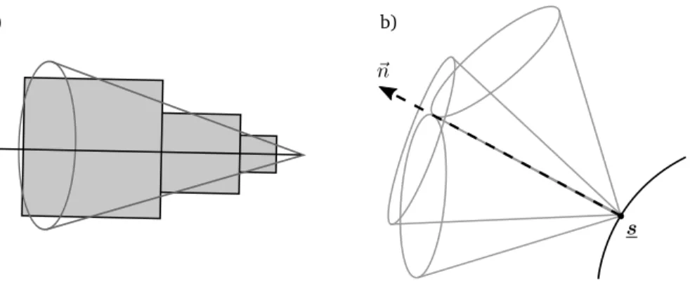
5.2.1 Focus Selection Bodies . . . 136
5.2.2 Glyph Shapes and Blur Kernels . . . 140
5.3 Algorithmic Details . . . 142
5.3.1 Approximative Kernel-Glyph Convolution . . . 143
5.3.2 Implementation Notes . . . 145
5.4 Interaction and User Interface Design . . . 147
5.5 Results . . . 149
5.5.1 Comparison to Color and Scale . . . 150
5.5.2 Case Studies . . . 153
5.5.3 Performance Evaluation . . . 161
5.6 Benefits and Limitations . . . 163
6 Discussion and Conclusion 167 6.1 Conformance to the Challenges . . . 169
6.2 Conclusion and Outlook . . . 173
Bibliography 177
1
Introduction
Particle-based simulations have been used in various sciences for decades [HE88]. They are an integral part of many research areas, such as meteorology, astro-physics, bioinformatics, medicine, thermodynamics or material sciences. Modern computers can run large-scale simulations with particle counts in the order of trillions. Each particle represents an individual entity that interacts with other particles and the constraints of the simulation space itself. This pushes the limits of what is possible to simulate, ranging from detailed representations on the molecular level [KS08] to gigantic systems, like the dark matter in the universe [Pot+17].
Ultimately, the purpose of a simulation is to gain insight, be it either to verify a hypothesis or to explore new models, parameters or constraints. Especially when a simulation is used for experimentation, it might be unclear what the result means. In this case, an automatic analysis that builds on abstraction is not usable since the underlying model is either unknown or cannot be formulated. At this point, at the latest, the human researcher is integrated into the loop to assess, evaluate and interpret the data. What is needed is a way to convey the relevant information, or, put in more mechanical terms, to transfer the information into the researcher’s brain as efficiently and correctly as possible. This is where scientific visualization comes into play. Following the definition of Earnshaw,
”scientific visualization is concerned with exploring data and infor-mation in such a way as to gain understanding and insight into the data. The goal of scientific visualization is to promote a deeper level of understanding of the data under investigation and to foster new insight into the underlying process, relying on the humans’ powerful ability to visualize” [Bro+12].
A successful visualization must adhere to three basic principles: expressiveness, effectiveness, and appropriateness. It isexpressive, if nothing but all relevant information is encoded [Mac86]. Aneffectivemapping from symbolic data to a visual representation exploits the capabilities of the output medium, and also that of the human’s visual system [Mac86]. If it balances the effort required for the visualization with the expected benefits it is considered to beappropriate
[SM99]. All requirements are intertwined and bound to two main limiting factors, the computational capabilities and the perceptual capabilities of the human observer.
Although Moore’s law slowly seems to come to a stop due to physical boundaries, computational power keeps increasing [Mac15]. With specialized hardware, such as dedicated graphics and computing cards, and an increasing parallel layout of computation units, particle visualization methods catch up to processing the arising massive amounts of data. Methods exist that show how to generate detailed renderings of particle datasets consisting of tens of billions of particles in interactive framerates using a specialized multi-core machine [Wal+15]. Methods that sacrifice detail even scale to trillions of particles [Sch+16]. The use of sophisticated optimized algorithms further lift the possibilities of what can be visualized, even on consumer hardware, making high-end visualizations widely accessible. The perceptual power of a human that means the maximum amount of information that the human researcher can comprehend, however, cannot be scaled in the same manner. Furthermore, visualizations of particle data, independent of their amount, face a number of unique challenges that, if not addressed impede understanding of the data.
1.1 Problem Statement
The ability to visualize more in the same computation time does in no way mean, that the user of such a visualization system can understand more. In fact, human visual perception and comprehension, although being undoubtedly very powerful, is limited, for example concerning the number of simultaneously trackable objects or the objective judgment of movement [Pyl+94; Bar01].
A second limiting factor is the limited resolution of the output medium. In a discrete visualization, showing more elements reduces the number of image elements that are available per particle, be it pixels or printed dots. Here, particle datasets are unique, since an increasing number of particles means that more entities must be shown. In contrast, when the resolution of volumetric data is increased, the spatial requirements do not grow in the same manner, since the volume that each voxel represents decreases. Especially, if a direct particle visualization is used that imposes as few assumptions as possible and thusshows
each particle individually, information is lost. In big datasets, individual particles are heavily undersampled, making them impossible to identify or distinguish. Falk et al. make the case, that a physical display does not allow to discern more particles than it has pixels since each particle must cover at least one pixel to be visible [Fal+16]. Methods exist to alleviate the issue by smoothing visual attributes along multiple particles, but they also reduce the visual separability of individual elements [Gro+10b].
Perhaps the most crucial factor that impedes comprehension lies in the nature of particle data itself. In many simulations, particles form dense clusters. Vi-sualizations that show particles as individual elements thus have to cope with heavy occlusion. Particle representations, especially if the underlying particle data has a grid-like layout, can completely block the view on the more interesting aspects that are happening in the inner. Furthermore, particles are not only defined by their position but a multitude of attributes. Their joint visualization is challenging, but essential to understanding all aspects. Also challenging is the fact that virtually all particle datasets are by design time-dependent which introduces an entire new dimension of complexity.
These perceptual bondaries and data-specific challenges define how much infor-mation can be encoded with one visualization approach. The only viable solution is to reduce the amount or the nature of the presented data. This can either be done by only showing a part of the data or by designing the visualization to show the particles at a coarser, more abstract level. For example, instead of focussing on the dynamics of individual particles, groups of particles that form structures, can be investigated.
This thesis aims to show possible solutions to the perceptual problem of particle visualizationsby integrating the concept of Focus+Context. The basic idea is to divide the data into two parts: a selected part, that is assumed to be interesting for a specific task, and the rest of the data. Instead of filtering the remaining data, i.e. removing it, it is kept in the visualizationin a reduced form with the purpose to support the selected data. Both, the selected and the remaining data are shownwithin the same visualization [Car+99]. The reduced form, called the context visualization, is presented such that it does not distract from the presentation of the selection, denoted asfocus visualization. The purpose of the context visualization is to help the user to understand the focus, that means, as the name suggests, to put the focus visualization into context. It is not a primary
goal of the context to contain detailed information, independent of the focus. This implies that perceptually simpler visualization forms must be chosen.
Using Focus+Context together with particle visualization has several advantages. First, the overall visual complexity is lowered. By allowing the user to visually focus on a manageable subset of the data, the visualization as a whole is effective. Second, complex and hidden structures become visible. Especially in particle data, dense structures cause occlusion or completely envelope relevant structures. For example, focussing on inner, otherwise occluded structures, makes them, by definition of a Focus+Context visualization, visible which allows gaining new insights. Third, since the context has looser constraints on expressiveness and accuracy, the design space for new visualizations is enlarged. The context needs to convey the information of its represented data only qualitatively. Note that of course a context visualization must remain meaningful, that means, it may not represent the data in a way that is implausible in the domain of the data’s origin. For example, reconstructing a Metaball surface from particles that repre-sent grains of sand might be a doubtable choice. Fourth, Focus+Context can be adapted to existing visualization approaches to lift their scalability. In essence, Focus+Context means two visualizations in one image. Although both visualiza-tions are ideally carried out using the same scheme, it is not mandatory. This means, existing methods can be declared to be either a focus or a context method, and only need a complementing second visualization. For example, instead of being forced to give up on a complex and visually demanding visualization for a large dataset, it can still be used to only show a selection of the data, while a perceptually simpler accompanying visualization shows the rest.
Designing viable Focus+Context visualizations is challenging in multiple ways. Ideally, such visualizations do not only have a focus or a context but also a transition. Its purpose is to connect the focus and the context in a continuous way to support comprehension. One of the central questions while conceiv-ing a continuous Focus+Context method is how this transition is carried out. Also, a Focus+Context visualization must be performant, since it copes with time-dependent data in a multi-dimensional space and thus most likely requires interactive control. Another open question is how the focus selection is carried out. Especially when dealing with higher dimensional data, this becomes challenging. In this work, several Focus+Context approaches for particle visualizations are shown. The presented methods cover the visualization of static particle data, time-dependent particle data, as well as multi-dimensional data.
1.2 Contributions and Thesis Organization
The remainder of this thesis is structured as follows. In the next chapter, the foundations of particle visualization and Focus+Context are laid out. section 2.2 presents a number of general challenges for a efficient, effective and appropriate particle visualization. Chapters 3 to 5 show three new methods for Focus+Context in particle visualization:Focus+Context is integrated into the classic splatting approach for static data. One of the basic methods for particle rendering is to show each individual particle as a solid sphere. Not only is this approach correct, in a sense that it visualizes the data, and nothing but the data, but it is also computationally efficient. It does, however, come with a number of shortcomings. Most importantly, it suffers from massive overdrawing, limiting the visiblity of inner structures. Also, essential features in the dataset, such as holes, rifts or valleys cannot be perceived due to the simple local lighting model. In chapter 3, an illumination model is pre-sented that consistently supports transparency and ambient lighting to enable a Focus+Context visualization. The transparency builds on the emission-absorption model known from volume rendering. In contrast to naive transparency, volumet-ric approaches help to preserve the three-dimensional impression of the glyphs. Using a modified version of approximate voxel cone tracing, based on a fast vox-elization of the particle data, and an analytic evaluation of the volume rendering integral interactive frame rates are achieved for static or dynamic datasets with particles in the order of millions. The benefits of the approach are presented on various real-world datasets where parts of the data are visually focused to be more detailed and salient.
Focus+Context is extended to time. Traditional visualization systems, while as-sisting to assess spatial features of the data, are typically based on animation to represent the time-dependent nature of the data. While this approach does have its benefits, it is heavily based on the human memory and lacks support for detailed time analyses. In chapter 4, the idea of Focus+Context is extended from space to time. This allows for a condensed visualization of spatial and temporal aspects in one static scene. The potential of such method is demonstrated on a simple example that shows one focused time step in detail while a selectable time span, the context, is shown in a more abstract manner, jointly in the same scene. Inspired by illustrative techniques, speed ribbons, adapted to the visualization of
larger particle structures, are employed. This allows assessing the time evolution around the temporal focus to gain insights on the cause and the effect of a distinct particle structure state, as is shown on several real-world datasets.
Focus+Context is applied to multi-dimensional particle data. In the presence of multi-dimensional data or if an unbiased visualization is desired, higher di-mensional visualizations are needed. In chapter 5, a method is presented that implements Focus+Context for multi-dimensional data. The basis is the scatter-plot matrix, which is known to introduce a high cognitive load since the data of each point is distributed over many panels. In order to facilitate cognition, more information from all dimensions is incorporated into each plot. At the same time, the visual load is reduced by using Focus+Context. The approach is based on a natural generalization of the depth-of-field effect from optics. A selection of the data comprises the focus that is shown sharply while the remaining data is blurred according to its distance to the selection. This allows for a continuous transition from focused data points, over regions of blurred points that provide contextual information to filtered data. The notion of focus selection bodies for data selection is introduced and various such bodies are presented and discussed. As shown on several case studies, depiction of higher order structures from only one plot, as well as encoding of additional useful information into the context, becomes possible.
In section 6, the presented approaches are discussed and evaluated for their conformance to the challenges listed in section 2.2. Finally, a conclusion is drawn and general ideas for future work are presented.
The chapters 3, 4 and 5 are based on the following papers. The contents were revised and heavily extended for this work.
• Joachim Staib, Sebastian Grottel, and Stefan Gumhold. ”Visualization of Particle-based Data with Transparency and Ambient Occlusion”. In: Computer Graphics Forum 34.3 (2015), pp. 151–160
• Joachim Staib, Sebastian Grottel, and Stefan Gumhold. ”Temporal Focus+Context for Clusters in Particle Data”. In: Vision, Modeling and Visualization (2017) • Joachim Staib, Sebastian Grottel, and Stefan Gumhold. ”Enhancing Scatterplots
with Multi-Dimensional Focal Blur”. In: Computer Graphics Forum 35.3 (2016), pp. 11–20
Additionally, the author contributed to the following works that are not discussed in-depth in this thesis:
• Dominik Vock, Stefan Gumhold, Marcel Spehr,Joachim Staib, Patrick Westfeld, H.-G. Maas ”GPU-Based Volumetric Reconstruction and Rendering of Trees From Multiple Images”. In: The Photogrammetric Record 27.138 (2012), pp. 175–194. • Joachim Staib, Marcel Spehr, and Stefan Gumhold. ”User Assisted Exploration
and Sampling of the Solution Set of Non-Negative Matrix Factorizations”. In: Proceedings of the IADIS Multi Conference on Computer Science and Information Systems (MCCSIS 2014) on Data Mining. Awarded best paper. Lissabon, Portugal: IADIS Press, 2014, pp. 29–38.
• Sebastian Grottel, Joachim Staib, Torsten Heyer, Benjamin Vetter, and Stefan Gumhold. ”Real-Time Visualization of Urban Flood Simulation Data for Non-Professionals”. In: Workshop on Visualisation in Environmental Sciences (EnvirVis). Ed. by Ariane Middel, Gunther Weber, and Karsten Rink. Cagliari, Italy: Eurograph-ics Association, 2015, pp. 037–041.
• Nico Schertler, Mirko Salm,Joachim Staib, and Stefan Gumhold. ”Visualization of Scanned Cave Data with Global Illumination”. In: Workshop on Visualisation in Environmental Sciences (EnvirVis). Ed. by Karsten Rink, Ariane Middel, and Dirk Zeckzer. The Eurographics Association, 2016.
• Sebastian Grottel, Patrick Gralka,Joachim Staib, et al. ”Visual and Structural Analysis of Point-based Simulation Ensembles” (IEEE VIS, Scientific Visualization Contest, Winning Entry). 2016.
• Sebastian Grottel, Christoph Müller, Joachim Staib, Thomas Ertl, and Stefan Gumhold. ”Extraction and Visualization of Structure-Changing Events in Molecular Dynamics Data”. In: Proceedings of TopoInVis Workshop 2017. 2017.
• Patrick Gralka, Sebastian Grottel,Joachim Staib, et al. ”2016 IEEE Scientific Visu-alization Contest Winner: Visual and Structural Analysis of Point-based Simulation Ensembles”. In: IEEE Computer Graphics & Applications (2017).
2
Fundamentals
This chapter outlines the fundamental ideas and concepts of particle visualization and Focus+Context. First, a basic definition of particle data itself, its sources and most prominent application areas is given. Then, fundamental rendering techniques are explained with a focus on the so calledbase-line sphere model. A variety of problems and requirements are presented that make the conception and implementation of particle visualization methods a challenging task. The second part of this chapter describes Focus+Context in more detail. In the last part, particle visualization and Focus+Context are combined by providing a condensed overview of existing literature in this field.
2.1 Particle Data and its Visualization
The core of a particle visualization is the underlying particle data. Formally, a single time step of a particle dataset is anunordered listPjofindividual objects
Pj= (p1, p2, ..., pl). (2.1)
Each particle is defined by an arbitrary, but constant number of attributes con-taining at least a position. Letpibe one particle as an element of an arbitrary attribute spaceA. Then
pi∈An+m (2.2)
whereAn+m consists ofnspatial coordinates and mfurther attributes. In the context of this work, let the position be real-valued. The complete attribute vector is thus defined as:
pi∈Rn×Am. (2.3)
Nearly all particle datasets contain multiple timesteps. Let for the sake of sim-plicity one particle list per time step exist. The entire particle dataset D is constituted by an ordered succession of independent particle lists to describe a time-dependent dataset withttime steps:
An element in a particle dataset represents anindependent objectof a simulation. Depending on the simulation and the employed model, a single particle can either represent anitem of a discrete simulationor be arepresentant of a continuous field. In discrete models, particles have a direct correspondence in the simulation, like an atom, a grain of sand or a bubble. Its attributes are valid individually for this particle and not for the surrounding space. As a consequence, an interpolation between particles is not meaningful. Still, it is possible to use the particles to derive measures of their surrounding space that are allowed to be interpolated. For example, the constellation and properties of molecules, each represented by a particle, allows defining a surface that is accessible to a solvent [Ric84]. Typically, the temporal development of individual particles is simulated to model the dynamics of the structure as a whole. This means, particles usually exist over multiple time steps and are thus spatially trackable. Nevertheless, depending on the simulation, particles can appear or vanish.
A particle in continuous models represents a discretization point of a continuous field. It does not have a direct correspondence to a single simulated object, but rather a group of objects or a portion of continuous space. As in discrete models, the individual particles interact over multiple time steps as independent objects. Whether the position of the particles changes when simulation time advances, depends on the used method. In Eulerian particle simulations, the positions do not change, but only the attributes. In Lagrangian particle models, the position changes with time [ZC07]. Mixed models exist which combine ideas of both methods. In contrast to discrete models, interpolation between particles is defined, as long as it is physically plausible. Particles in continuous models must not be confused with mere sample points of data, that was not produced by particle simulations. This includes point clouds, acquired by scanning or sampled data from simulations using different techniques. Of course, situations exist where it makes sense to also visualize non-particle data with particle visualization methods. For example, the award-winning entry for the IEEE SciVis contest 2016 built on a particle visualization [Gro+16]. The given dataset was the result of a Finite Pointset Method, whose elements do not necessarily allow an interpretation as particles.
The number of spatial parameters defines the dimensionality of the simulation’s physical domain. Note that the spatial dimensionality is not equal to the dimen-sionality of the dataset. In contrast to, for example, volumetric data which is truly three-dimensional data, particles form a list where the position is not an
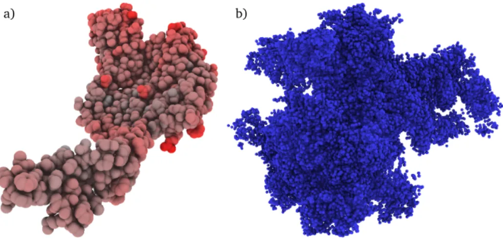
a) b)
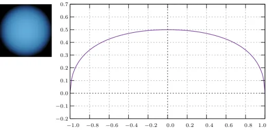
Fig. 2.1: Examples of base-line visualizations with ambient occlusion. (a) Visualization of the protein with PDB ID 1UUN. (b) Visualization of a synthetic particle structure.
independent variable. That means, it is not possible to freely chose a position in this dataset, because it is only defined at exactly the positions of the particles. As a consequence, a particle dataset is in fact zero-dimensional. If elements of the particle list can be accessed by an index, the dataset can be referred to as being one-dimensional, and if it is time-dependent, as being two-dimensional. Although this distinction as such is of minor relevance for this thesis, a crucial fact of particle data is reflected: the particle’s position is not more than a subset of many attributes. Obviously, since it represents the physical domain, the position is of major importance but does not define the state of the particle alone. It is the entire set of attributes that steer the interaction and evolution of particles. In fact, when the data stems from a Eulerian simulation where positions are fixed, other attributes must be incorporated in order to understand the data. This fact is important when designing anunbiasedparticle visualization, as will be shown in chapter 5. This work focusses on visualizing the particles as individual objects, as shown in Figure 2.1. For item-based simulations, this scheme is straightfor-ward. If the particle data stems from a continuous model, a visualization of the underlying continuous structure, for example, a volume or a surface, might seem more natural. However, showing individual objects per particle is not wrong in this case, but shows the data as-is, without employing reconstruction schemes or deriving other attributes. It thus makesminimal assumptionson the data. While not being as intuitive, it is advantageous to, for example, evaluate simulation algorithms or directly observe particular particles and their evolution. Falk et al.
refer to this general visualization scheme asbase-line rendering[Fal+16]. The authors state that it is especially useful for visual debugging, i.e. the possibility to check simulation results on a small scale. Ideally, a base-line rendering serves as a starting point in the communication with domain experts, being as close to the raw dataset as possible.
2.1.1 Particle Simulation Methods and Application Areas
During the last decades, myriads of particle-based simulation techniques in differ-ent scidiffer-entific areas have evolved, too numerous to give an exhaustive overview. All methods build on the same principle: the simulated matter is described as a set of independent entities. The purpose of the simulation is to calculate an evolution of a system or structure over time by expressing the system’s dynamics as interactions between particles, as well as additional external effects [HE88; Mon92]. As mentioned, particle simulations can roughly be categorized into discrete and continuous techniques, depending on whether the particle represents an individual item or a packet of a continuous field. They can furthermore be cate-gorized into deterministic and stochastic methods. In deterministic models, as the name suggests, the evolution is entirely defined by the initial conditions, i.e. given the same initial attributes, the simulation outcome will be the same. Stochastic models are used to include uncertainty and probability rates. Events happen with a given probability, making these simulation methods non-deterministic. They are for example used to simulate models that contain stochastic events themselves, like quantum dynamics, or when a single particle represents a set of objects with differing behavior. In the following, prominent discrete and continuous techniques are presented, and typical applications are outlined.
Molecular Dynamics Simulation and Discrete Element Method
Being one of the fundamental methods for discrete simulations, the Molecular Dynamics (MD) method is used to simulate dynamics on an atomic scale. It was first described by McCammon in order to investigate protein folding processes and was since adapted and transferred to other areas [McC+77]. Each particle is modeled as a mass element without a specific shape to represent an atom or molecule. During simulation, particles induce forces on neighboring particles, for example by atomic force fields or pairwise potentials. All forces are added to yield
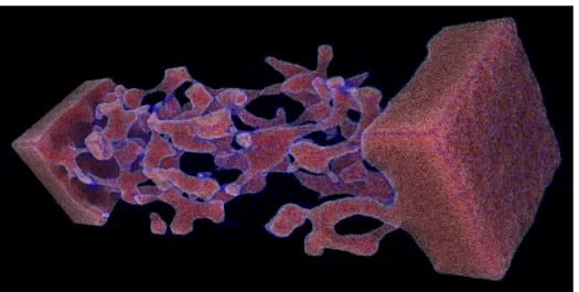
a) b)
Fig. 2.2: Examples of discrete particle simulations. (a) Visualization of a nucleation process. The excerpt shows local heterogeneity in homogeneous nucleation in the proximity around a large grain (Figure from [Shi+17], Fig. 7). (b) Visualization of a small porous media sample made from distinct polyhedra-shaped particles (Figure from [Gro+10a], Fig. 1).
the evolution of all particles in one time step. Typically, the motion is defined by Newtonian equations of motion. The interactions model a time span in the order of femtoseconds. That means a full simulation run might contain several million time steps in order to cover a time span of a few hundred nanoseconds. The simulation results yield essential information on the smallest scale. They serve, in a generalized manner, as input for higher scale simulations.
Nowadays, MD simulations are used in various fields, not only restricted to biology or chemistry but also physics, engineering or material sciences. One interesting use case is in thermodynamics to simulate nucleation. This term describes the localized formation of a distinct thermodynamic phase in another phase. It is of high significance in order to understand the formation of crystals in liquids or the process of liquefaction in vapors [Tan+11]. Figure 2.2 (a) shows a small portion of a larger dataset during nucleation. Visualization of the simulation outcome is mostly carried out using aggregated and more abstract visualizations, for example, line plots. They are typically accompanied by direct visualizations of individual points, see [KM02] for an example.
Another prominent use, especially in physics, engineering and chemistry is the analysis of nano droplets. They play a key role in many fields, for example for the development of hydrophobic surfaces or to study the behavior of fuel
droplets in car engines, to name only a few. Research includes effects of the droplets themselves, like evaporation and deformation when exposed to different media and, more importantly, interactions with surfaces or other droplets [JB08]. For example, when a droplet of a liquid contacts a surface, it either wets it, deforms to a sessile droplet or, in the case of hydrophobic surfaces can bounce off [GM07]. The specific deformation and interaction with the surface deliver significant insight into the design and properties of these surfaces. The collision of a droplet with other droplets can have multiple effects. One effect, a deformation and diffusion, is shown in one of the evaluation datasets used in section 3.6.1 and section 4.6.1.
Many other use cases exist, for example in material sciences. MD methods in this field are for example used for the analysis of lattice and defect dynamics. Nearly all materials have a variety of defects and other features on a microscopic level. For example, crystalline materials have dislocations and point defects. Their investigation is especially useful for product design and testing [SH09]. Another relevant use case is the study of laser ablations in anorganic and organic material. By simulating a laser pulse, energy is injected into a simulated matter, leading to the ejection of molecules. Simulated laser impacts with a duration in the order of femtoseconds are used in various applications, such as micromachining or the generation of nano diamond clusters [Son+11]. In this thesis, two different simulations of laser ablations in anorganic matter are used in the evaluation in section 3.6.1 and section 4.6.2. The laser ablation scenario is furthermore used for example in surgery to simulate the removal of biological tissue, for ionization experiments or fabrication of polymer films [ZG99].
As mentioned, MD is the cornerstone of a variety of derived simulation techniques. One popular extension is the so calledDiscrete Element Method(DEM). In contrast to MD that treats particles as mass centers, DEM considers the particle’s shape. Particles have an actual geometry, for example, spherical or polyhedral, as shown in Figure 2.2 (b). The attribute space is extended to also contain shape parameters, mass centers and additional state variables like rotation. The Interaction between particles is accordingly extended to include stateful contacts [Zhu+08]. This opens possibilities for simulations in various fields, where particles represent for example sand [Fin+16], powder [Mar+03] or other geomaterials [Don+09]. For visualization, it is beneficial to consider this shape. Extended visualization algorithms exist, for example for grains that are modeled using a polyhedral model [Gro+10a].
a)
b)
c)
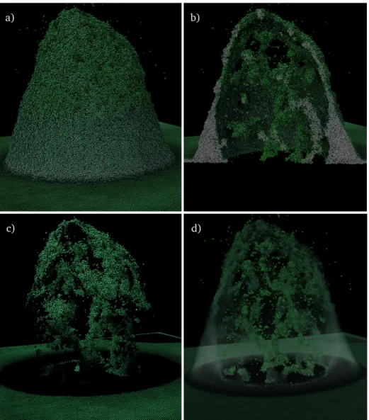
d)
Fig. 2.3: Examples of continuous particle simulations. (a) Particle distribution in one time step of a shallow water simulation. (b) Surface reconstruction of the same distribution (Figure (a) and (b) from [LH10], Fig. 5). (c) Visualization of the Dark Sky n-Body simulation (Figure from [Sch+16], Fig. 1). (d) Detailed closeup of a dark matter simulation using tetrahedrons to preserve details (Figure from [Kae+12], Fig. 5).
Smoothed Particle Hydrodynamics and n-Body Simulations
One fundamental technique to simulate continuous models is the Smoothed Particle Hydrodynamics (SPH) method. It was initially developed to approximate the continuum dynamics of fluids in order to study phenomena in astrophysics [Mon92]. As a Lagrangian method, each particle represents a discretized part of the continuum that moves over time. It is especially appealing for its ease to use while delivering accurate results. It allows simplifying the complex equations in hydrodynamics to formulations of comparably simple equations for the interaction of particles [Mon92]. Most importantly, the method conserves energy, momentum, mass, and entropy. SPH is used for the simulation of models that describe the formation and dynamics of galaxies, stars or planets. This involves solving complex gas dynamics, coupled with various fields, like radiation or magnetic fields. Recent works take the full cosmological context into account, based on
inflationary theory [Spr10]. This allows simulating the formation of disk galaxies and even spiral galaxies. Also, SPH is used to study the generation and basics of magnetic fields or cosmic rays.
On smaller scales, SPH is used in many areas, for example in solid mechanics to simulate impact problems or metal forming, in fluid dynamics to study heat conduction or underwater explosions, or in wave impact studies on offshore structures [Cre08]. SPH is also used for presentation, for example, to simulate plausible water behavior in interactive applications. By not showing the particles themselves, but a derived translucent and refracting surface, a realistic water effect is achieved. For real-time applications, the problem can be reduced to two dimensions to simulate the behavior of shallow water, as shown in Figure 2.3 (a) and (b) [Bar+11].
Related to SPH, but based on the laws of Newtonian gravity are n-body simu-lations. They have become especially popular in astrophysics to study the time evolution of dark matter. The most prestigious projects in this area are the so-called Millenium Simulations [BK+09]. In 2005, the first simulation, often referred to as Millenium Run, was carried out. It simulates the cluster formation of dark matter over a period of 14 billion years. Beginning with a nearly uniform placement of approximately 10 billion particles, each representing one billion solar masses of dark matter, the universe’s evolution is tracked in steps of little more than one million years, yielding about 11,000 time steps in total. The simu-lated area covers a cubical area with a length of 2 billion light years. Subsequent simulations were Millenium II and Millenium XXL. The Millenium II simulation covers a space of about 400 million light years, again with approximately 10 billion particles, thus achieving a higher resolution. Millenium XXL, performed in 2010, covers a cube with a side length of more than 13 billion light years. The simulation was carried out using about 300 billion particles, each representing 7 billion solar masses [Ang+12]. Although being impressive in numbers, Millenium XXL is not the biggest simulation of dark matter. It was outrun by the Horizon Run 3, with 370 billion particles, the DEUS FUR simulation with 550 billion particles and the DarkSky simulation with over 1 trillion particles [Kuh+12]. Figure 2.3 (c) shows a visualization of the data. More recently, Potter et al. have completed the largest dark matter n-Body simulation, involving 2 trillion particles [Pot+17]. Due to the high amount of data, visualization approaches in this field give up on showing each individual particle. Instead, visualizations based on aggregate information and subsampling are used [Sch+16].
2.1.2 Rendering Approaches
A wide variety of problem-specific rendering approaches for particle data exist. The purpose of this section is to give a condensed overview of fundamental techniques and to describe the base-line approach for this thesis in greater detail. For a comprehensive review on particle visualization techniques, please refer to the recent state of the art report on biomolecular visualization by Kozlíková et al. and the more general review by Falk et al [Koz+16; Fal+16].
One of the fundamental visualization method for particle data is glyph-based visualization [Gro12]. The idea is to represent each particle with a distinct geometric object, the glyph, that allows depicting multiple particle attributes [Bor+13]. Each glyph is independent of other glyphs, as is the case in the original data. What glyph represents a particle best depends on the particle’s physical model. Especially for the visualization of molecular dynamics simulations, the calotte model is commonly used. For each atom, a hard sphere represents its position and the van der Waals radius, i.e. the radius of the minimally possible interatomic distance [Bat01]. Because of their simplicity and comparably efficient visualization, hard spheres are also used in other particle domains.
With the advent of dedicated graphics processing units, interactive three-dim-ensional visualizations of large particle counts became possible. Early methods were bound to the comparably inflexible programming pipeline and thus used triangulated approximations of hemispheres, oriented towards the virtual camera. Since the spherical surface is approximated with linear segments, visual artifacts emerge, especially on the silhouette. To alleviate this problem, high triangle counts needed to be generated per sphere which impacts performance [Gro+10b]. Methods exist that use multiple levels of detail, depending on the distance of the sphere to the image plane [Hal+05]. In the early 2000s, graphics units became more flexible by introducing shader programs that enable execution of arbitrary code at defined stages in the graphics pipeline. This allowed for more accurate and faster rendering techniques.
One of the first techniques using more modern graphics card features was based on advanced precomputed sphere textures that were used as billboards. For each particle, a quadrilateral polygon is generated and accordingly textured [Baj+04]. Rather than colors, as was the only possibility with the fixed function hardware, the texture contains normal and depth information to allow for proper lighting and
c b1 b3 b4 b2 f ~ d
Fig. 2.4: Raycasting of spherical glyphs. First, a quadrilateral is generated (defined by the four pointsb1...4) that tightly approximates the sphere, given a perspective camera with camera pointc. For each fragment of the quadrilateral during rasterization, a ray is constructed and tested for intersection with an implicit formulation of the sphere. If the ray intersects the sphere, the fragment is colored accordingly, otherwise it is discarded.
manipulation of the depth buffer. This strategy, however, suffered from artifacts when the screen size of one sphere is bigger than the original texture or when the texture’s bit depth is not sufficient [Gro12]. The latter was indeed a problem at the time, where only textures with 8 bit per channel were supported. Also, the billboards suffered from incorrect perspective distortion. When a perspective camera is used, spheres appear as ellipsoids at the camera image’s edges. This is especially important to plausibly convey relative positions and touching spheres when a perspective virtual camera is used for the visualization. A superior ray-casting based approach, that does not require precomputed textures and is considerably faster on modern hardware was proposed by Gumhold in 2003 [Gum03]. This approach is a fundamental component in the methods described in chapter 3 and 4 and thus explained in more detail in the following.
Sphere Rendering by Raycasting
Similar to the texture-based approach a quadrilateral is generated for each sphere glyph. During rasterization, instead of sampling from the texture, the fragment’s color is determined by a ray-intersection test of a viewing ray from the virtual
c c c0 b 0 1 b02 a) b) b2 b3 b1 b4
Fig. 2.5: Determination of tight silhouette quad. (a) Four planes from the camera point
cform a frustum and each plane tangentially touches the sphere in one of the pointsb1...4. (b) Every two points lie on a plane that is perpendicular to thexz, respectivelyyzplane (not shown) in camera space. Projecting the camera point on the plane reduces the problem of finding each two of the tangent points to two dimensions.
camera through the fragment and an implicit formulation of the sphere. If the ray intersects the sphere, a normal vector is calculated for shading, and a depth value is obtained to set the depth buffer. If no intersection occurs, then the fragment is discarded. Figure 2.4 illustrates the strategy.
This approach has various benefits. First, the silhouette is pixel perfect accurate up to floating point precision. Second, it is fast, since it does not require any texture lookups, but only a small number of arithmetic evaluations. Third, it scales well, because the needed computational time for one sphere depends on the number of pixels that the sphere covers. This means, when many small spheres are to be rendered, the computation time for a single sphere decreases. Performance can further be improved by generating the quadrilateral such that the number of fragments that need to be evaluated is minimal. Fourth, in contrast to using textures, perspective projection is handled correctly.
The detailed rendering pipeline is as follows. First, a quadrilateral is generated that tightly fits to the sphere’s silhouette in screen space. In camera space, i.e. in the 3d space before perspective projection, this polygon is a rectangle. It is obtained by the observation, that because of the perspective view, the visible part
0 b01 b02 c0 p p h h r r ~ v α β β
Fig. 2.6: Geometric construction to find two of the four silhouette points (on one of the two axis aligned planes, see Figure 2.5 (b) for a reference). In total, the camera pointc0, the silhouette pointb01, the sphere center in the origin and another pointpallow constructing three nested triangles.
of the sphere is bound by a pyramidal frustum with planes thattangentiallytouch the sphere at one point each [Rei08]. These four points constitute the extents of the tight silhouette quad. Figure 2.5 (a) illustrates this concept. Without loss of generality, let the sphere be centered in the origin. Since a sphere is rotationally symmetric, the problem can be formulated such that every two of the points lie on a plane that is parallel to thexz plane, respectivelyyzplane in camera space. Both planes contain the sphere’s center. Thus, two points each can be found by only considering their respective two-dimensional plane, as illustrated in Figure 2.5 b). For each of the two planes, the two touching points can be determined using a geometric construction. Figure 2.6 shows the construction in thexzplane. In the figure, the two sought two-dimensional pointsb01andb02are the tangential touching points of the circle with radiusr. Thus, in Figure 2.6 two symmetric right triangles can be constructed. The pointsb01andb02are obtained by moving punits from the sphere’s center in direction to the camera, i.e. in negative direction~v(and become pointp) and thenhunits in the perpendicular direction. Since the problem is 2D, obtaining the perpendicular direction to~vis straightforward.
The pointpis obtained by p=0+p· ~v k~vk (2.5) andpis calculated as p= r 2 k~vk. (2.6)
This is due to the fact that the right triangles t1 = 0c0b01 (red) andt2 =0pb01 (green) share a common angleα. Int1, the angleαcan be computed ascos(α) =
r
k~vk and in t2, αis computed ascos(α) = pr. Combining both equations and solving forpleads to Equation 2.6. The remaining sought value forhcan then be calculated in the trianglet2following Pythagoras’ laws as
h=pr2−p2. (2.7)
Reina proposes to calculatehinstead byh=√pqwithq=k~vk −p[Rei08]. This is a more practical solution if the quantityqis needed for other purposes since it saves computations for the calculation ofhcompared to Equation 2.7. The equation can be obtained by the fact, that the trianglest2(green) andt3=pc0b01 (purple) share a common angleβ. This is due to the fact that both triangles have a right angle and the common angleα. Similar to Equation 2.6, the angleβ is calculated int2 astan(β) = hp and int3astan(β) = hq. Again, combining both equations and solving forhyields the desired equation. Fromp, movinghunits in perpendicular direction of~vyields b01 and moving in the opposite direction yieldsb02. An analog calculation can be performed in theyzplane to obtain the remaining two points.
During rasterization of the rectangle, a raycasting of the implicit sphere surface is performed. First, the fragment’s coordinates are transformed to glyph space, that means a space where the sphere is in the origin. Then, a ray is constructed from the camera positioncthrough the fragment’s position. Letf be the 3d position of the fragment in glyph space, then the ray is defined by the foot pointcand the directiond~=kf−ckf−c (cf. Figure 2.4) as
r(t) =c+t ~d. (2.8)
The implicit formulation of a pointxon a sphere centered at the origin with radiusrreads
Inserting Equation 2.8 into Equation 2.9 yields
0 = Dc+t ~d,c+t ~dE−r2 (2.10)
= (cx+t·dx)2+ (cy+t·dy)2+ (cz+t·dz)2−r2 (2.11)
Exploiting the fact, thatkdk~ = 1, the ray parameter of the closest intersection is calculated as tn=− D c, ~dE− r r2− hc,ci+Dc, ~dE2. (2.12) Adding the term under the square root instead of subtracting it yields the ray exit positiontf. This is especially relevant for the transparent ball glyphs as presented in chapter 3.
The ray does not intersect the sphere if the termr2− hc,ci+Dc, ~dE 2
is smaller than zero. Inserting the result in Equation 2.8 yields the intersection point which is used to calculate the normal and depth of the sphere surface point.
On modern GPUs, most of the work, such as the rasterization is done by the graphics pipeline itself. A vertex shader program must merely calculate the required touching points to define a quadrilateral. In practice, a quadratic point primitive can be used that, although not tightly bounding the silhouette, is faster, since only one vertex per sphere must be defined [Fal+16]. In the fragment program, the intersection test must be carried out, followed by simple local lighting calculations. This allows even naive implementations to achieve interactive framerates for particles in the order of hundreds of millions. More optimized algorithms can show billions of sphere glyphs on commodity hardware in real-time [Gro+10b].
Other Visualization Techniques
Many other visual representations exist, which are highly problem and data specific. For example in chemistry and biology, other depictions than the calotte are common, such as the Ball-and-Stick representation. Atoms are visualized with spheres which are connected by cylindrical elements that represent bonds. Similar to sphere glyphs, the cylinders can be efficiently and accurately calculated on graphics hardware using raycasting [Gro12]. A simpler form that omits the spheres entirely is the Stick representation. In cases where views on entire
molecules are more relevant than views on individual atoms, more complex structures can be represented using a single glyph, for example again using a sphere to show a molecule that is composed of multiple atoms. In the case of molecules with more than one mass center, composed glyphs can be used. For example, elements with two mass centers can be efficiently rendered by placing one sphere per mass center and additionally showing a dipole moment by using a two-colored cylinder [RE05]. If only a polarization is to be shown, simpler glyphs are available, for example, arrow glyphs that consist of a cylinder and a cone [Gro12].
Especially, when the particle simulation itself assumes a specific shape on the particle or when additional parameters are encoded, specialized glyphs are useful. For example in the Discrete Element Method, particles can be represented as polyhedra. Reflecting these shapes during visualization can be efficiently done with modern graphics hardware by using tesselated primitives and instancing [Gro+10b]. Alternatively, raycasting approaches exist that evaluate intersections with the polyhedron’s tangent planes and determine the union of the correspond-ing half-spaces.
Methods exist that do not show individual particles but rather represent a set of particles as continuous structures. This makes sense when derived measures are visualized or when the particles itself represent discretizations of a continuous matter. One prominent example is the aforementioned n-body simulation of dark matter. Visualization methods in this area seek to overcome problems related to the vast amounts of data. One of the first works that visualized the Millenium Run dataset was by Hopf and Ertl [HE03]. Particles are splatted using anti-aliased points. Based on the distance, coarser resolutions of the dataset are splatted, such that one point represents multiple particles of the dataset. A later work by Kaehler et al. adheres more to the physical properties of the data [Kae+12]. It is based on a reconstruction and visualization of the dataset using tetrahedrons. This way, the method can retain subtle details, like filaments. Schatz et al. targeted even bigger datasets and proposed a method to visualize the DarkSky simulation with over one trillion particles [Sch+16]. They use a combination of per-particle splats and volume rendering.
Especially for continuous simulations, visualizations exist that build on conveying the density distribution using volume rendering techniques. In a preprocessing step, the dataset is voxelized into a volumetric data structure. While this
ap-b)
c) a)
Fig. 2.7: Examples of surfaces from particle data. (a) The metaball surface shows spherical glyphs in proximity as a connected surface (Figure from [Mü+07], Fig. 8). (b) Van-der-Waals surface of a protein (PDB ID 2ONV). (c) The solvent excluded surface defines the boundary for external atoms that do not intersect any atom of the molecule (Figures (b) and (c) from [Kro+09], Fig. 2).
proach allows the subsequent use of standard volume rendering algorithms, it is limited by the resolution of the voxel grid and the imposed memory requirements [Fal+10]. Other methods do not show a volume but reconstruct a surface. This makes it possible to only reconstruct the needed surface information on the fly, instead of computing the entire volume. Each particle represents the center of a distribution, for example by a Gaussian kernel. An implicit function is obtained by summing over all kernels. From this function, a surface can either be recon-structed by indirect methods, such as Marching Cubes, or by direct methods, for example raycasting. One popular example is the generation of Metaball surfaces [Bli82]. Figure 2.7 (a) shows an example. Methods in these fields can be divided into object space methods and image space methods. While the latter can be carried out without preprocessing, the performance depends on the screen resolu-tion, rather than the data. More importantly, these methods introduce artifacts [Mü+07]. Especially in molecular dynamics simulations, derived surfaces like the Solvent Accessible Surface or Solvent Excluded Surface (SeS) are visualized , as shown in Figure 2.7 (b) and (c) [Alh+17]. Intuitively, they are generated by rolling off a sphere over all atoms and trace the rolled-off surface. The SeS can be efficiently constructed by concatenation of a small set of geometric primitives. Since molecular dynamics simulations typically contain thousands of time steps,
a precomputation in each frame is costly regarding computation time and mem-ory requirements. It is, however, possible to generate these surfaces on the fly by raycasting implicit representations of the contributing geometric primitives [Kro+09].
2.2 Challenges in Particle Visualizations
Visualizing complex, time dynamic particle datasets in an effective, efficient and appropriate manner is a challenging tasks. In the following, critical challenges are explained in more detail. They serve as the basis to assess the quality and success of the here-proposed Focus+Context techniques. The challenges are divided into three groups. Structural challenges are concerned with the structure and distribution of the particle data itself. Temporal challenges are related to visualization requirements that arise due to the time-dependent nature of the data.Algorithmic challengesdescribe the most important problems that an implementation of a particle visualization system must be able to solve.
C1. Structural Challenges
Particle data bears a variety of unique challenges concerning the distribution of the particles and the intention of a visualization. Relevant aspects exist not only on a per-particle level, but only on multiple structural levels simultaneously. Typically, these structures are dense and thus introduce occlusion.
C1.1. Relevant aspects exist on multiple scales. A particle dataset is usually the result of a particle simulation. As outlined in section 2.1.1, each particle is simulated individually as an element of higher-order structures. Typically, relevant aspects happen on the per-particle level, as well as on the level of the higher-order structures. For example, it might be interesting for a scientist to observe the deformation of nano droplets as a whole. At the same time, intersting effects happen on the particle level, for example in the form of evaporation or diffusion. A key aspect to understand the data is the fact that effects on multiple scales affect one another. For example, a nano droplet can change its shape or volume depending on evaporation and diffusion. Multiple scales can also exist on the level of higher order structures itself, for example, when connected particle clusters
Fig. 2.8: Visualization of one time step from the ”Bursting Liquid Layer” dataset (cf. dataset D5 of section 3.6). Note the many different scales of the dynamic structures, beginning from single particles up to clusters that contain 100,000s of particles.
detach from a larger cluster, they can be of arbitrary particle count magnitudes. Figure 2.8 shows a particle dataset of a liquid layer of argon in a vacuum that is ripped apart as a consequence of the applied pressure. Note the many different scales between the emerging clusters. Ideally, a particle visualization is able to
convey information from multiple scales simultaneously.
C1.2. Structures are dense. With few exceptions, particle simulations incorpo-rate some notion of attraction between particles. Be it based on Newtonian laws of movement in molecular dynamics simulations or laws of gravity in n-body simulations. Sooner or later this causes dense structures. They can become problematic in spatial visualizations, since they introduce occlusion. A typical remedy is to make the visualization interactive, i.e. letting the user gain control over a virtual camera. This interactivity resolves cases where dense structures block other structures only from certain viewing positions. It does, however, not help when such structures completely envelope other possibly relevant parts of the dataset. In this case, the user must be provided with more advanced tools to clear the view. A particle visualization that is aware of this requirement thus incorporates a means ofrevealing occluded structures, preferably without removing data that might be valuable.
C1.3. Particles can have a multitude of additional parameters. The particles in a dataset are not only defined by their position but exist in a space with arbitrary additional dimensions. Particle data should bevisualized including all relevant attributes, ideally in an unbiased fashion. This is challenging, since the number of concurrently perceivable attributes is limited. Basic spatial mappings that use spherical glyphs map the particle’s position to the glyph position, the most defining force to the radius and can then usually map only one more additional attribute to the color, without introducing potential interference of visual attributes.
C1.4. Particles are true independent entities. In discrete simulations, particles are true independent entities, rather than, for example, a sample from a continu-ous field. This discerns particle visualizations from other techniques, like voxels in volume rendering. Derived surfaces only make sense when they are semantically plausible and should thus be used with caution to represent the data. Ideally, a particle visualization, especially when it aims to convey the data simulation process represents asingle particle as visible, distinguishable objectand only uses derived surfaces and abstractions when necessary and plausible. This challenge is related to C1.1 (Relevant aspects on multiple scales) but restricts its design space to favor visualizations that convey higher order structures as compounds of distinguishable particle objects.
C2. Temporal Challenges
Particle data is usually time-dependent, that means it consists of multiple time steps. During its evolution, the higher order structures can change drastically and rapidly. On the per-particle level, the movement is typically not smooth, but subject to micro movements.
C2.1. Particle data is usually time-dependent. Particles evolve by successive in-teraction and evolution. Depending on the simulation method, many discrete time steps are required until interesting dynamics and effects emerge. For example, in molecular dynamics simulations one time step covers a time span in the order of femtoseconds while an entire simulation run typically covers a time span of multiple nanoseconds. N-body simulations like the Millenium Run have time steps in the order of up to millions of years, but cover a total time span of billions of years. Typically, what is interesting for the scientists in this data is not only the
Fig. 2.9: 20 random particle paths from the Colliding Droplets dataset (cf. case study D3 of section 3.6 and case study 1 in section 4.6.1). The particles have a trending direction but are subject to heavy micro movement, induced by collisions. After the droplets impact, complexity of the path further increases.
particle state at one time step but the temporal development. Thus, a particle visualization must in some wayintegrate the concept of temporal exploration.
C2.2. Particle structures are highly dynamic. In contrast to other data domains, structures in particle data can change drastically over time. This is due to the fact that these clusters consist of many small independent elements that are bound by inter-particle forces. Structural changes can be induced by many reasons, such as strong external forces or events like collisions, or merging and splitting of structures. For a visualization, this makes it hard, if not impossible, to approximate higher order structures correctly over time using static geometry. For example in one of the datasets used in the evaluation in chapter 3 and 4, three droplets approach and then collide. While at first having an almost spherical shape the collision introduces a spontaneous drastic deformation. The droplets only slowly return to a more regular shape after the collision. A particle visualization must thus beaware of the possibility of slow or spontaneous changes of clusters.
C2.3. Particles are subject to micro-movements. Usually, the path of a single particle is not smooth, but affected by micro movements. They can be caused by collisions with other particles, be explicitly modeled effects like Brownian Motion or be the result of temporal simulation sampling. In fact, usually not all time steps during a simulation run are saved for later visualization. This leads to a
massively undersampled particle path which makes acorrectreconstruction of the particles path virtually impossible. Especially for derived and more abstract visualizations, it is thus challenging to obtain stable and reliable aggregates. For example, Figure 2.9 shows the paths of20particles of a molecular dynamics simulation being subject to heavy micro movements. One solution would be to simplify the motion and, as a last resort, to use smoothing. This, however, removes information for the visualization that is intentionally part of the data. A particle visualization should berobust against micro movementswhen calculating aggregate values. If an unaltered mapping of the data is desired a visualization should includemeans to convey micro movements qualitatively, as well.
C3. Algorithmic Challenges
Since particle data is stored in an unordered list, advanced queries need additional data structures that require memory and computation time to generate. Also, for a particle visualization to be interactive, it should exploit caches wherever possible. This, however, is challenging, because particle data consists of many independent, unaligned data packets.
C3.1. Particle data is typically an unordered list. Unlike volume data or vector field data that is often stored in a regular grid, particle data is usually represented as an unordered list of individual particles. Since a dataset contains particle counts in the order of up to trillions, additional acceleration data structures are inevitable to query data relations. One class that is especially important is neighborhood queries. They are, for example, required for advanced rendering effects, density estimation or collision detection. What data structure should be used depends on the required query precision, memory requirements and the available computational time budget. A particle visualization must incorporate andefficiently generate and evaluate appropriate acceleration data structures.
C3.2. Particle data consists of short, scattered information packages. Usually, a single particle contains information in the order of tens to hundreds of bytes. Since one cannot assume an order on the individual particles in the list, elements that are neighbors in the particle list are not required to be spatial neighbors. Rendering approaches that work directly on unordered lists thus either have non-aligned write or read accesses, thus are not able to exploit fast cache memory. Especially when repeatedly writing data to graphics card buffers, exploiting write
caches can be crucial to maintaining acceptable performance. One time step may contain gigabytes of particle data, so high throughput is essential. Ideally, a performant particle visualization thus performs an adequate reordering of the elements, if needed, toexploit CPU and GPU caches.
C3.3. Particle data lives in a possibly cyclic space. Most particle visualizations assume a finite, but boundless simulation space. This is achieved by introducing cyclic border conditions, i.e. particles that leave the simulation space on one side reemerge on the opposite side. This might not be a problem for the visual repre-sentation of the data itself, especially when it also explicitly shows boundaries of the simulation space. Cyclic border conditions must, however, be considered for the calculation of aggregated measures or to build acceleration structures. A particle visualization must thusaccount for possibly cyclic bordersand select appropriate algorithms for the calculation of derived or interpolated attributes.
2.3 Foundations of Focus+Context
Focus+Context methods aim to improve the visibility of data visualizations. The main idea is to split the visualization into two parts: the focus and the context. The focus comprises the currently interesting data and is rendered in full detail to allow for aprecise analysis. The remaining data, the context, is shown within the same visualization, but in a reduced form tosupport the focus. Its purpose is to put the focus into the context of the complete dataset. What part of the data is the focus and what is the context, is based on a data selection, which is either explicitly done by the user or implicit, according to queries on features in the dataset.
Focus+Contex has its origins in Information Visualization and can be traced back to the early 1980s. In 1981, Furnas presented a technique for the efficient display of text [Fur81]. The purpose of his work was to better exploit the limited possibilities of text displays. A part of the data is considered more important, based on the data structure itself, as well as on the user interaction. Textual information in focus is devoted the majority of screen space. Depending on the distance to the focus, text is devoted less screen space. Comparing this paradigm to a wide angle fisheye-lense from optics, Furnas states that ”by considering these two contributions, the ’fisheye view’ represents an effort to balance [...] the need
Fig. 2.10: Perspective Wall method by Apperley et al. [App+82]. Data in focus is shown unaltered with increasing perspective distortion to the left and right of the focused region.
for local detail against the need for global context”. Three parameters steer this approach: a focal point, a problem specific distance from the focus and a level of detail that is applied to every data element depending on the distance. As will be shown later, these are, in an extended manner, also the three main ingredients of modern Focus+Context applications.
In 1982, Apperley et al. presented a related method that was intended for graphics displays [App+82]. To overcome the ”window problem”, the fact that a display can only show a window of the data, the authors suggested splitting the display horizontally into three parts. The center shows the currently selected part of the data structure, while the left and right third of the screen show data parts to the left or right with increasing minification towards the vertical screen borders. The authors compare this idea with a scroll that rolls over two parallel bars. Figure 2.10 shows a recreation of this concept. The idea to distort the graphical data display using the fisheye metaphor depending on a user selectable importance was since adopted to numerous works. For example, in 1992, Sarkar et al. presented a fisheye view for graphs [SB92]. Their main observation was that details might become too small to be adequately depictable in complex visualizations. Similar to a magnification lens, a selected node of a graph is magnified. Other nodes appear successively smaller depending on the number of edges to the focus. Since the space requirements of the nodes vary interactively, the graph is heavily distorted. Figure 2.11 shows another example of the fisheye view in medical volume rendering.
a) b) c)
Fig. 2.11: Example for fisheye distortion in volume rendering. (a) The distortion mask magnifies a radial part of the visualization. (b) Unaltered medical volume visualization. (c) Applied fisheye effect with the focus on an aneurysm. (Figures (b) and (c) from [CB04], Fig. 6.)
Using distortion to overcome the windowing problem seemed to be an effective means, so research in this area blossomed. In order to consolidate recent works, Leung and Apperley presented a taxonomy of distortion-based techniques in 1994 [LA94]. This taxonomy classified visualization techniques into distorted and non-distorted views. While non-distorted views allow showi