Using adaptively weighted large margin classifiers for robust sufficient dimension reduction

This is an Open Access document downloaded from ORCA, Cardiff University's institutional

repository: http://orca.cf.ac.uk/123584/

This is the author’s version of a work that was submitted to / accepted for publication.

Citation for final published version:

Artemiou, Andreas 2019. Using adaptively weighted large margin classifiers for robust sufficient

dimension reduction. Statistics 53 (5) , pp. 1037-1051. 10.1080/02331888.2019.1636050 file

Publishers page: https://doi.org/10.1080/02331888.2019.1636050

<https://doi.org/10.1080/02331888.2019.1636050>

Please note:

Changes made as a result of publishing processes such as copy-editing, formatting and page

numbers may not be reflected in this version. For the definitive version of this publication, please

refer to the published source. You are advised to consult the publisher’s version if you wish to cite

this paper.

This version is being made available in accordance with publisher policies. See

http://orca.cf.ac.uk/policies.html for usage policies. Copyright and moral rights for publications

made available in ORCA are retained by the copyright holders.

Using adaptively weighted large margin classifiers for

robust sufficient dimension reduction

Andreas Artemiou

School of Mathematics, Cardiff University

Abstract

In this paper we combine adaptively weighted large margin classifiers with Support Vector Machine (SVM)-based dimension reduction methods to create dimension reduction methods robust to the presence of extreme outliers. We discuss estimation and asymptotic properties of the algorithm. The good perfor-mance of the new algorithm is demonstrated through simulations and real data analysis.

Key Words: Dimension reduction; adaptive weights; Support Vector Machines; Outliers

1

Introduction

Nowadays, high dimensional problems are becoming the norm due to the increase of computing power and storage capabilities. At the same time classic statistical tech-niques, which were developed based on low dimensional problems, lack the ability to generalize and perform robustly in high dimensional problems. One way to overcome this difficulty is to perform dimension reduction to our data before applying any of the traditional techniques to it.

Sufficient Dimension Reduction (SDR) is a class of techniques for supervised fea-ture extraction in a high dimensional regression (or classification) setting. In SDR we assume that we have a univariate (without loss of generality) response variableY and a p dimensional predictor vector X. Our objective is to estimate a set of dfeatures (where d_≤p) without losing information on the conditional distribution ofY_|X. In other words, we are trying to estimate a p_×dmatrixβ which satisfies

Since the extracted features are linear functions of the original predictors this is called linear SDR. The space spanned by the columns ofβis called the Dimension Reduction Subspace (DRS). The intersection of all possible DRSs if it is itself a DRS it is called the Central Dimension Reduction Subspace (CDRS) or simply the Central Subspace (CS) and it is denoted with _SY|X. CS is the space that has the smaller dimension (d) among all DRSs. Although the CS doesn’t always exist the assumptions required for existence are mild so for the rest of the paper we assume existence of the CS (see Cook - 1998a). Classic methods in the SDR literature have been proposed in Li (1991), Cook and Weisberg (1991), Li (1992), Cook (1998b), Li, Zha, Chiaromonte (2005) and Li and Wang (2007) among others.

More recently, Li, Artemiou and Li (2011) have proposed Principal Support Vec-tor Machine (PSVM) which uses previous ideas in the SDR framework as well as Support Vector Machine (SVM) to achieve dimension reduction. The most impor-tant advantage of this algorithms is that it provides a common framework for linear and nonlinear SDR. Artemiou and Shu (2014) applied a cost based reweight technique which improved the performance of the algorithm as it was taking into account the imbalanced nature between the slices. Moreover, Shin et al (2014, 2017) have used weights to estimate a probability enhanced CDRS when the response is binary.

In this work, we are interested to develop a method that is robust to the presence of extreme outliers. Towards this, we introduce adaptive weights in the objective function of PSVM. To achieve this, we use the idea by Wu and Liu (2013) where adaptive weights are used to improve the classification performance of SVM (the most well-known large margin classifier). Wu and Liu (2013) proposed a two-run method. In the first run, they solve the optimization problem to obtain a first estimate of the optimal separating hyperplane. Then they suggested using a second run to find the final estimate of the optimal separating hyperplane. In the second run though they suggested to use the misclassification distance of the misclassified points as an inverse weight in the optimization problem. In the SDR framework, we propose to take a similar approach with Wu and Liu (2013) to improve the estimation performance of PSVM for dimension reduction. The new algorithm is called Adaptively Weighted Principal Support Vector Machine (AWPSVM). Further to this, we also apply the adaptive weights to Principal L2 SVM (PL2SVM) which was proposed by Artemiou and Dong (2016) and it was demonstrated that it generally has better performance than PSVM. Finally, although the theoretical framework of our methodology is similar to the one by Shin et al (2017) who used weighted SVM to achieve dimension reduction on binary responses, we emphasize that there are important differences. First of all,

we have a different objective as we are targeting extreme outliers while they target dimension reduction when the response is binary. Furthermore, our methodology slices the response, which is not the case for Shin et al (2017).

The rest of the paper is organized as follows. In section 2 we discuss PSVM and other similar existing methodology and we introduce AWPSVM in section 3. In section 4 we discuss some asymptotic properties. In section 5 we present some simulation results and real data analysis follows in section 6. A small discussion closes the paper.

2

Previous work

In this section we discuss briefly different methods that were introduced in the SVM-based dimension reduction literature and which are related to the method we are proposing in this work. For the rest of the section suppose (Xi, Yi) i = 1, . . . , n

independent observations. LetΣ= var(X) and assume that the support ofY can be split in two disjoint sets A1 and A2 so that we define ˜Y =I(Y ∈A2)−I(Y ∈A1).

2.1 Principal Support Vector Machine (PSVM)

PSVM (Li, Artemiou and Li -2011) minimizes the following objective function: L(ψ, t) =ψT_{Σψ+λE{1−Y}˜_[ψT_{(X −EX)−t]}}+

, (2)

where λis the misclassification penalty (or cost as it is known in the machine learn-ing literature) and a+_{= max}

{0, a_} . Also (ψ, t)_∈Rp×Rdefine the equation of the separating hyperplane. The objective is to find a pair of (ψ∗, t∗_)∈Rp_×Rwhich

min-imizes the objective function (2). At the sample level the authors (roughly) suggested the use of different cutoff points qk, k = 1, . . . , h to construct multiple hyperplanes

described by ( ˆψ∗_i,ˆt∗_i), i = 1, . . . , h. Then an eigenvalue decomposition of the ma-trix ˆM =Ph_i=1ψˆ

∗

i( ˆψ

∗

i)T will give us the eigenvectors corresponding to the largest d

eigenvalues, where dis the estimated dimension of the CS.

2.2 Principal Lq Support Vector Machine

PSVM algorithm in Li, Artemiou and Li (2011) gave a unique solution of the optimal hyperplane in terms of the normal vectorψ. This, though, was not true for the offset t. Therefore, Artemiou and Dong (2016) proposed the use of Lq Principal Support Vector Machine (LqSVM) in sufficient dimension reduction. The objective function

in this case is:

L2(ψ, t) =ψTΣψ+E{(1−Y˜[ψT(X−EX)−t])+}2, (3)

where we have a strictly convex function that can ensure the uniqueness of the optimal hyperplane in both ψ and t. Although tis not used in the estimation of the CS, as one can see in both Li, Artemiou and Li (2011) and Artemiou and Dong (2016) it is important on the development of the asymptotic theory as different quantities (i.e. Hessian matrix and therefore asymptotic variance) depend on it’s value.

2.3 Principal Weighted Support Vector Machine

Shin et al (2017) presented the following idea to achieve sufficient dimension reduction in cases with binary response:

LW(ψ, t) =ψTΣψ+λE{π(Y)(1−Y[ψT(X−EX)−t])}+, (4)

where π(Y) = 1₋π and π _∈ (0,1). They incorporated weights using the idea of weighted SVM (see Lin et al (2002)) to estimate the CS. Here we emphasize that their method mainly tackles cases where there is binary response. Classic SDR methods cannot estimate more than one direction whenever the response is binary. On the other hand, the use ofπ-path trajectories in the weighted SVM algorithm helps avoid this issue in Shin et al (2017).

2.4 Cost Reweighted Principal Support Vector Machine

Artemiou and Shu (2014) presented another form of weighted algorithm. Their ob-jective was to accommodate for cases where there was imbalance in the number of observations between the two disjoint sets A1 and A2 of the support of Y. The

objective function in this case is:

LCR(ψ, t) =ψTΣψ+E{λ_Y˜(1−Y˜[ψT(X−EX)−t])}+, (5)

where the only difference from the PSVM method is the dependence of the misclassi-fication penaltyλon the value of ˜Y to show that the two classes have different costs. Again the objective of this algorithm was to use cost based reweighting to target bias introduced due to imbalance and not to address the presence of extreme outliers as we do in this case.

3

Adaptively weighted algorithms for SDR

In this section we propose adaptively weighted versions of PSVM from Li, Artemiou and Li (2011) and Principal L2SVM from Artemiou and Dong (2016). To achieve this we use the adaptively weighted SVM idea in Wu and Liu (2013).

3.1 Adaptively Weighted Principal SVM

Adaptively Weighted Principal Support Vector Machine introduce weights into the objective function. This weights are carefully chosen so that extreme outliers, and more specifically points that are incorrectly classified and further away from the separating hyperplane, get a smaller weight and their importance is downplayed. The objective function takes the form

LAW(ψ, t) =ψTΣψ+λE{w(1−Y˜[ψT(X−EX)−t])+}, (6)

where for this work we assume that w >0 (we will discuss the choice of the weights in the estimation section). Also notice how there is a similarity of this with both the weighted algorithms discussed in the previous section.

In the next theorem we show that indeed one can use theψ∗_∈Rpto estimate the CDRS. The proof is similar to the respective theorems in Li, Artemiou, Li (2011), Artemiou and Shu (2014) and Shin et al (2017).

Theorem 1 Suppose E(X_|βT_{X) is a linear function of β}T_{X, where β is as defined}

in (1). If (ψ∗, t∗_{) minimizes the objective function (6) among all (ψ, t) ∈ R}p_×R,

then ψ∗_{∈ SY|X}.

Proof. _{From the population version in (6) let’s assume without loss of generality}

that E(X) = 0 so it becomes

LAW(ψ, t) =ψTΣψ+λE{w(1−Y˜[ψTX −t])+}. (7)

Since w > 0 then E_{w(1₋Y˜[ψT_{X −t])}+

} = E_{w(1₋Y˜[ψT_{X −t])}}+_{. Thus, the}

population version in (7) is equivalent to:

LAW(ψ, t) =ψTΣψ+λE{w(1−Y˜[ψTX −t])}+. (8)

Now note that:

E_{w(1₋Y˜[ψT_{X −t])}}+

=E_{E_{w(1₋Y˜[ψT_X−t])}+

Since the functiona_7→a+

is convex, by Jensen’s inequality we have E_{[w(1₋Y˜(ψT_X −t))]+_|Y,βT_X } ≥{E[w(1₋Y˜(ψT_X −t))_|Y,βT_X] }+ =w[1₋Y˜(E(ψT_X |βT_X) −t)]+, where the equality follows from Y X_|βT_{X. Now we can use the following}

E_{w[1₋Y˜(ψT_X

−t)]_}+_≥E_{w(1₋Y˜[E(ψT_X |βT_X)

−t])_}+. (9) Also, note that

var(ψT_{X) = var[E(ψ}T_X|βT_{X)] +E[var(ψ}T_X|βT_{X)]≥var[E(ψ}T_X|βT_{X)]. (10)}

Combining (9) and (10), we see that

L(ψ, t)_≥var[E(ψT_X|βT_{X)] +λE{w(1−Y}˜_[E(ψT_X|βT_X)−t])}+

. (11) Note that E(ψT_X

|βT_{X) = ψ}T_PT

β(Σ)X where (Pβ(Σ) is the projection matrix

β(βT_Σβ)−1_βT_{Σ) which implies that the right hand side of (11) is simplyL(P}

β(Σ)ψ, t).

That is, for every ψ_∈Rp,

L(ψ, t)_≥L(Pβ(Σ)ψ, t). (12)

If ψ does not belong to _SY|X, then var(ψTX|ηTX) >0, and the inequality in (10)

become strict. Hence the inequality in (12) is strict. Therefore, suchψ cannot be the

minimizer ofL(ψ, t). _✷

3.2 Adaptively Weighted Principal L2SVM

When one introduces weights in the Principal L2SVM algorithm then the objective function takes the following form:

ΛAW L2(ψ, t) =ψTΣψ+λE{w[(1−Y˜[ψT(X−EX)−t]) +

]2_}. (13) It is then easy to prove the following theorem.

Theorem 2 Suppose E(X_|βT_{X) is a linear function of β}T_{X, where β is as defined}

in (1). If (ψ∗, t∗) minimizes the objective function (13) among all (ψ, t) _∈Rp ×R, then ψ∗_{∈ SY|}X.

The proof is omitted as it is similar to the one for the Adaptively Weighted PSVM in the previous section as well as Theorem 1 in Artemiou and Dong (2016).

4

Estimation

In this section we discuss how we construct the estimation algorithm for the adaptively weighted algorithms proposed in the previous section.

4.1 Adaptively Weighted Principal SVM

To propose the estimation algorithm for the adaptively weighted PSVM, we first write the sample version of the objective function (6), that is:

ˆ LAW(ψ, t) =ψTΣnψ+ λ n n X i=1 wi{1−Y˜i[ψT(Xi−X)¯ −t]}+. (14)

Then one needs to standardize the predictors using Zi = Σ− 1/2

n (Xi−X¯) and ζ =

Σ1n/2ψ and the objective function becomes:

ˆ LAW(ζ, t) =ζTζ+ λ n n X i=1 wi{1−Y˜i[ζTZi−t]}+. (15)

This looks similar to the adaptively weighted large margin classifier objective function proposed by Wu and Liu (2013) in the classification framework. We first solve (15) based on the quadratic programming problem suggested by the following Theorem and then use the minimizer ζ∗ to estimate ψ∗ = Σ−n1/2ζ∗ which is the minimizer

of (14). Also, note that _⊙ is used to denote the elementwise multiplication of two vectors of the same size, i.e. for vectors a = (a1, . . . ak) and b = (b1, . . . , bk), then

a_⊙b= (a1b1, . . . , a_kb_k).

Theorem 3 If ζ∗ minimizes the objective function in (15) over Rp, then ζ∗ =

1

2Z

T_{(α⊙y˜) where α is found by solving the quadratic programming problem:}

maximize αT₁ −1₄(α_⊙y˜)T_ZZT_(α ⊙y˜) subject to 0< α < λ nw, (α⊙y˜) T_{1= 0.} (16) where 0= (0, . . . ,0), 1= (1, . . . ,1)T_∈Rn _{and w= (w} 1, . . . , wn)T.

Proof. _{Using similar developments as in Vapnik (1998) one can show that}

mini-mizing (15) is equivalent to minimizing ζT_ζ+λ nw T_{ξ over (ζ, t,ξ)} subject to ξ_≥0, ξ _≥1₋y˜_⊙(ζT_Z −t1) (17)

where ξ= (ξ1, . . . , ξn). The Lagrangian function of this problem is L(c, t,ξ,α,β) =ζT_ζ+ λ nw T_ξ −αT_[˜y ⊙(ζT_Z −t1)₋1+ξ]₋βT_{ξ. (18)}

If (ζ∗,ξ∗, t∗_{) is a solution to problem (17) then using Karush-Kuhn-Tucker Theorem,}

one can show that minimizing over (ζ, t,ξ) is similar as maximizing over (α,β). So, differentiating with respect to ζ,t, and ξ to obtain the system of equations:

         ∂L/∂ζ = 2ζ₋ZT_(α ⊙y˜) =0 ∂L/∂t=αT_{y˜= 0} ∂L/∂ξ= λ_nw₋α₋β=0 (19)

Substitute the last two equations above into (18) to obtain ζT_ζ

−αT_(˜y

⊙(ζT_Z)

−1). (20)

Now substitute the first equation in (19) (ζ = 1

2Z

T_{(α⊙y˜)) in the above:}

1T_α

−1₄(α_⊙y˜)T_ZZT_(α

⊙y˜). (21)

Thus to minimize (18) we need to maximize (21) over the constraints

   αT_y˜=0 λ nw−α−β=0 (22)

which are equivalent to the constraints in (25). ✷

The above result can be then used to construct the following algorithm: 1. Compute the sample mean ¯X and sample variance matrix ˆΣ=n−1Pn

i=1(Xi−

¯

X)(Xi−X¯)Tand use them to standardize the data and set weightswi = 1, i=

1, . . . , n

2. Letqr, r= 1, . . . , H−1, beH−1 dividing points. In the simulation section we

choose them to be, the (100_×r/H)th sample percentile of _{Y1, . . . , Yn}. For

each r, let ˜Y_ir = I(Yi > qr)−I(Yi ≤ qr) and use Theorem 3 to find (ˆζr,ˆtr)

be the minimizer of (15) where ˜Yi is replaced with with ˜Yir and weightswi are

replaced withwr

i = 1 fori= 1, . . . , n. This process yieldsH−1 normal vectors

ˆ

ζ1, . . . ,ζˆH−1.

4. For each dividing pointqr calculate

wr_i = 1

1 +_|ψT

r(Xi−EXi)−tr|

.

5. Using the weights wr_i in the previous step repeat steps 2 and 3 to find ˆψw_r, r= 1, . . . , H₋1 (new estimate of the coefficients based on the weights).

6. Construct matrix ˆVn=PH_r=1−1ψˆ w rψˆwr

T

.

7. Let ˆv1, . . . ,ˆv_d be the eigenvectors of the matrix ˆV_n corresponding to its d

largest eigenvalues. We use subspace spanned by ˆv = (ˆv1, . . . ,vˆd) to estimate

the CDRS, _SY|X.

The above algorithm is based on the “left vs right” (LVR) idea proposed by Li, Artemiou and Li (2011). It can be easily transformed to the “one vs another” (OVA) idea proposed in the same paper.

4.2 Estimation for Adaptively Weighted Principal L2SVM

A similar argument as the one used in the previous section gives us the estimation algorithm for adaptively weighted PL2SVM. One needs to show that the following Theorem holds. We omit the details due to the similarity of the arguments. First we need to write the sample version of the objective function in (13) as:

ˆ LAW L2(ψ, t) =ψTΣnψ+ λ 2n n X i=1 wi({1−Y˜i[ψT(Xi−X)¯ −t]}+)2. (23)

Then if we standardize the predictors usingZi=Σ− 1/2

n (Xi−X¯) andζ =Σ 1/2 n ψthe

objective function becomes: ˆ LAW L2(ζ, t) =ζTζ+ λ 2n n X i=1 wi({1−Y˜i[ζTZi−t]}+)2. (24)

We first solve (24) based on the quadratic programming problem suggested by the following Theorem and then use the minimizer ζ∗ to estimate ψ∗ =Σ−n1/2ζ∗ which

is the minimizer of (23).

Theorem 4 If ζ∗ minimizes the objective function in (24) over Rp, then ζ∗ =

1

2Z

T_{(α⊙y˜) where α is found by solving the quadratic programming problem:}

maximize αT₁ −1₄(α_⊙y˜)T ZZT₊2n λ D −1 w (α_⊙y˜) subject to 0< α, (α_⊙y˜)T_{1= 0} (25)

The proof of Theorem 4 is similar to the one in the previous section and therefore it is omitted. The same can be said in the estimation algorithm where the only difference is in Step 2 where one can modify it to the following:

Letqr, r= 1, . . . , H−1, beH−1 dividing points. In the simulation section

we choose them to be, the (100_×r/H)th sample percentile of_{Y1, . . . , Yn}.

For each r, let ˜Yr

i = I(Yi > qr)−I(Yi ≤qr) and use Theorem 4 to find

(ˆζ_r,ˆtr) be the minimizer of (24) where ˜Yi is replaced with with ˜Yir and

weights wi are replaced with w_ir= 1 for i= 1, . . . , n. This process yields

H₋1 normal vectors ˆζ1, . . . ,ˆζH−1.

4.3 Asymptotic theory

Following similar developments to Li, Artemiou and Li (2011) and Artemiou and Dong (2016), one can derive the asymptotic result of the adaptively weighted algorithms. We list here only the main results for the adaptively weighted Principal L2SVM algorithm which we list without proofs as these are similar to the ones that appear to Artemiou and Dong (2016). It is important to remind here that the weights are assumed non-random.

First of all we assumeE(X) =0without loss of generality and we use the notation θ = (ψT_{, t)}T_{,Z= (X}T_,Y˜₎T_,X† _{= (X}T_,

−1)T _{and Σ}†_{= diag(Σ,0), where diag(A,B)}

denotes a block diagonal matrix withAandBon the block diagonals. Also note that λ†_=λ2−1

w wherew is the weight. Λ(ψ, t) in (13) can be rewritten asE_{m(θ,Z)_}, where

m(θ,Z) =θT_Σ†_θ+λ†_{(1−θT_XY˜₎+

}2

. (26)

Comparing this with the respective expression for the asymptotics of PL2SVM in Artemiou and Dong (2016) the only difference is that λ† includes the weight as well. This explains why the asymptotic results for the adaptively weighted method is similar to the asymptotic results of PL2SVM.

Note that we denote withEn{m(θ,Z)} the corresponding sample version of the

objective function and we define θ0 and ˆθ to be the minimizers of E{m(θ,Z)} and

En{m(θ,Z)} respectively. The next theorem gives the the gradient function of the

L2 objective function E_{m(θ,Z)_}. To prove it one will need the prove of Lemma 1 of Artemiou and Dong (2016).

Proposition 1 Suppose for each y˜_{∈ {−}1,1_}, the distribution of X_|Y˜ = ˜y is domi-nated by the Lebesgue measure. In addition, suppose E(_kX_k2) <_∞ and E(_kX_k)<

∞. LetDθbe the(p+1)-dimensional column vector of differential operators(∂/∂θ1, . . . , ∂/∂θp+1)T.

Then

Dθ[E{m(θ,Z)}] =(2ψTΣ,0)T

−2λ†EnX†Y˜h(1₋θT_X†_Y˜_)I(1

−θT_X†_{Y >}˜ ₀₎io_{. (27)}

The next proposition finds the Hessian matrix ofθ. To prove it one will need to use Lemmas 2 and 3 in Artemiou and Dong (2016).

Proposition 2 SupposeX has a convex and open support, and for eachy˜_{∈ {−}1,1_}, the distribution of X_|Y˜ = ˜y is dominated by the Lebesgue measure. Let f_·|· denote the conditional probability density function. Suppose, moreover:

1. for any linearly independent ψ,δ_∈Rp, y˜=₋1,1, and v, ǫ_∈R, the function u_7→y˜(1₋y˜(u₋t)₋ǫv)E_{X†_|ψT_{X =u,δ}T_{X =v,Y}˜ _{= ˜y}

}∗ ∗fψTX|δTX,_Y˜(u|v,y˜)

is continuous;

2. for anyi= 1, . . . , p, and y˜=₋1,1, there is a nonnegative function ci(v,y˜) with

E_{ci(V,Y˜)|Y˜}<∞ such that

˜

y(1₋y˜(u₋t)₋ǫv)E_{Xi|ψTX =u,δTX =v,Y˜ = ˜y}fψTX|δTX,_Y˜(u|v,y˜)

≤ci(v,y˜);

3. for anyy˜=₋1,1, there is a nonnegative functionc0(v,y˜)withE{c0(V,Y˜)|Y˜}<

∞ such thatfψTX|δTX,Y˜(u|v,y˜)≤c0(v,y˜).

Then the function θ_7→Dθ[E{m(θ,Z)}]is differentiable in all directions with

deriva-tive matrix

H = 2diag(Σ,0) + 2λ†H† (28)

where H†=P ˜

y=−1,1P( ˜Y = ˜y)E{X†(X†)TI(1−θTX†y >˜ 0)|Y˜ = ˜y}

The next result finds the influence function of ˆθ.

Theorem 5 Suppose the conditions in Propositions 1 and 2 are satisfied. Then ˆ

θ=θ0−H−1Dθ0[E{m(θ0,Z)}] +oP(n

−1/2

),

Now let’s define some notation that will help us define the asymptotic normality of the candidate matrix ˆV. First, for a fixed dividing point qr, we have ˜Yr, r =

1, . . . , H ₋1 to be the discretized responses. Then we can define Zr = (XT_,Y˜r_),

m(θ,Zr) =θT_Σ†_θ−λ†_{(1−θT_X†_Y˜r₎+

}2

and letθ0r= (ψT0rt0r)Tbe the minimizer of

E_{m(θ,Zr)_}overθ. The population version of ˆV in the estimation algorithm is thus V =PH_r=1−1ψ0rψT0r. LetKp,p be the unique matrix satisfyingKp,pvec(A) = vec(AT)

for anyA_∈Rp×p,Frbe the firstrrows ofHr−1 withHr the Hessian ofE{m(θ,Zr)}

and denotes_r(θ,Zr) =FrDθ0[E{m(θ0,Z)}]. Using this notation one can define the

asymptotic distribution as follows:

Theorem 6 Suppose the conditions in Propositions 1 and 2 are satisfied. Then

√_{nvec( ˆV}

−V) converges to multivariate normal with mean0and varianceΛ1Λ2Λ1,

were Λ1 =I_p2 +K_p,p and Λ2= H−1 X r=1 H−1 X i=1 [ψ0rψT0i⊗E{sr(θ0_r,Zr)sT_i(θ0_i,Zi)}].

Let ˆU = (ˆu1, . . . ,uˆd) be the population version ofU = (u1, . . . ,ud), whereu’s are

the dleading eigenvectors of V. LetD be a diagonal matrix with diagonal elements being the d leading eigenvalues of V. The following corollary gives the asymptotic distribution of ˆU and it can be proved using Corollary 1 in Bura and Pfeiffer (2008).

Corollary 1 Suppose the conditions in Propositions 1 and 2 are satisfied, andV has rank d. Then

√

nvec( ˆU ₋U)_−→D N 0,(D−1UT

⊗Ip)Λ1Λ2Λ1(D−1UT⊗Ip).

5

Simulation

In this section we run some simulations to show the improved performance of the proposed methodology. We run simulations for the following models:

Model I: Y =X1+X2+σε,

Model II: Y =X1/[0.5 + (X2+ 1)2] +σε,

Model III: Y =X1(X1+X2+ 1) +σε,

where X _∼ N(0,I_p×p), p = 10,20,30, ε _∼ N(0,1). There are 100 simulations with sample size n= 100. We have the number of slices H = 20 (we run for H = 50 as

well but the results were similar and therefore we omit them). Finally, σ = 0.2 and the misclassification penaltyλ= 1.

To compare the performance of the algorithm we use a metric proposed by Li, Zha, Chiaromonte (2005). Let _S1 and S2 be two subspaces of Rp and PS1, PS2 the

orthogonal projections on them respectively. Then the distance is measured by the matrix norm

dist(_S1,S2) =kPS1−PS2k. (29)

Using the true and estimated space as the two subspaces in the formula then the above measures the distance between them. The smaller the distance the best performance of the algorithm. In our simulations we are using the Frobenius norm.

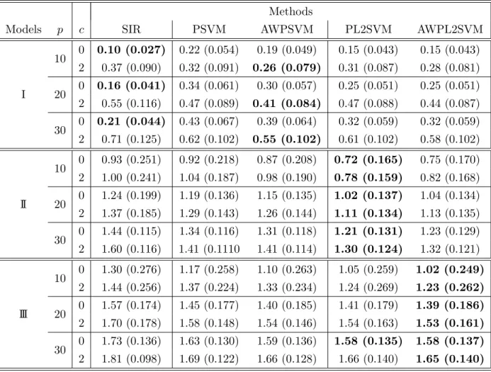
In Table 1 we can see the results of the 4 algorithms (PSVM, PL2SVM and their adaptively weighted versions) for H = 20 and different values of p when there are no outliers (c = 0, where c denotes the number of extreme outliers) and when there are two (c = 2) extreme outliers in the dataset. We also included SIR in our comparisons to compare with the performance of traditional methodology in the presence of extreme outliers. Those extreme outliers are created by taking the two points with the smallest responseY. We force them then to have the largestY in the dataset by changing the sign ofY. This ensures that these two points are constantly outliers in every left vs right (LVR) comparison we apply in the dataset. As we can see there is almost always better performance of the adaptively weighted version of the two algorithms even when there are no outliers (with the exception of the PL2SVM algorithm in model 2 but even in that case the performance is close). We see that the difference between the algorithms diminishes asp gets larger. To help the reader in visualizing the performance of the algorithm, in each scenario we put in bold the algorithm that has the best performance.

6

Real data analysis

We use the airfoil self-noise dataset in the UC Irvine Machine Learning repository (Dua and Karra Taniskidou - 2017). This is a NASA dataset, obtained from a series of aerodynamic and acoustic tests of two and three-dimensional airfoil blade sections conducted in an anechoic wind tunnel and it consists of 1503 observations with 5 predictors (Frequency, Angle of attack, Chord length, Free-stream velocity, Suction side displacement thickness) and one response variable (scaled sound pressure levels). We run PSVM and PL2SVM and the adaptively weighted versions of them, with 5 and 20 slices. The results are similar and therefore we present the ones with 5

Table 1: Mean and standard deviation (in parentheses) of the Frobenius norm for PSVM (Li, Artemiou and Li - 2011), PL2SVM (Artemiou and Dong - 2016) and the adaptively weighted versions of the two algorithms (denoted as AWPSVM and AWPL2SVM for H = 20. The value of c denotes the number of extreme outliers in the 100 points

Methods

Models p c SIR PSVM AWPSVM PL2SVM AWPL2SVM

I 10 0 0.10 (0.027) 0.22 (0.054) 0.19 (0.049) 0.15 (0.043) 0.15 (0.043) 2 0.37 (0.090) 0.32 (0.091) 0.26 (0.079) 0.31 (0.087) 0.28 (0.081) 20 0 0.16 (0.041) 0.34 (0.061) 0.30 (0.057) 0.25 (0.051) 0.25 (0.051) 2 0.55 (0.116) 0.47 (0.089) 0.41 (0.084) 0.47 (0.088) 0.44 (0.087) 30 0 0.21 (0.044) 0.43 (0.067) 0.39 (0.064) 0.32 (0.059) 0.32 (0.059) 2 0.71 (0.125) 0.62 (0.102) 0.55 (0.102) 0.61 (0.102) 0.58 (0.102) II 10 0 0.93 (0.251) 0.92 (0.218) 0.87 (0.208) 0.72 (0.165) 0.75 (0.170) 2 1.00 (0.241) 1.04 (0.187) 0.98 (0.190) 0.78 (0.159) 0.82 (0.168) 20 0 1.24 (0.199) 1.19 (0.136) 1.15 (0.135) 1.02 (0.137) 1.04 (0.134) 2 1.37 (0.185) 1.29 (0.143) 1.26 (0.144) 1.11 (0.134) 1.13 (0.135) 30 0 1.44 (0.115) 1.34 (0.116) 1.31 (0.118) 1.21 (0.131) 1.23 (0.129) 2 1.60 (0.116) 1.41 (0.1110 1.41 (0.114) 1.30 (0.124) 1.32 (0.121) III 10 0 1.30 (0.276) 1.17 (0.258) 1.10 (0.263) 1.05 (0.259) 1.02 (0.249) 2 1.44 (0.256) 1.37 (0.224) 1.33 (0.234) 1.24 (0.269) 1.23 (0.262) 20 0 1.57 (0.174) 1.45 (0.177) 1.40 (0.185) 1.41 (0.179) 1.39 (0.186) 2 1.70 (0.178) 1.58 (0.148) 1.54 (0.146) 1.54 (0.163) 1.53 (0.161) 30 0 1.73 (0.136) 1.63 (0.130) 1.59 (0.136) 1.58 (0.135) 1.58 (0.137) 2 1.81 (0.098) 1.69 (0.122) 1.66 (0.128) 1.66 (0.140) 1.65 (0.140)

Table 2: Mean and standard deviation (in parentheses) of the distance of the direction found when imposing extreme outliers to the airfoil data from the “oracle” direction

Methods

PSVM AWPSVM PL2SVM AWPL2SVM

● ● ● ● ● ● ● ● ● ● ● ● ● ● ● ● ● ● ● ● ● ● ● ● ● ● ● ● ● ● ● ● ● ● ● ● ● ● ● ● ● ● ● ● ● ● ● ● ● ● ● ● ● ● ● ● ● ● ● ● ● ● ● ● ● ● ● ● ● ● ● ● ● ● ● ● ● ● ● ● ● ● ● ● ● ● ● ● ● ● ● ● ● ● ● ● ● ● ● ● ● ● ● ● ● ● ● ● ● ● ● ● ● ● ● ● ● ● ● ● ● ● ● ● ● ● ● ● ● ● ● ● ● ● ● ● ● ● ● ● ● ● ● ● ● ● ● ● ● ● ● ● ● ● ● ● ● ● ● ● ● ● ● ● ● ● ● ● ● ● ● ● ● ● ● ● ● ● ● ● ● ● ● ● ● ● ● ● ● ● ● ● ● ● ● ● ● ● ● ● ● ● ● ● ● ● ● ● ● ● ● ● ● ● ● ● ● ● ● ● ● ● ● ● ● ● ● ● ● ● ● ● ● ● ● ● ● ● ● ● ● ● ● ● ● ● ● ● ● ● ● ● ● ● ● ● ● ● ● ● ● ● ● ● ● ● ● ● ● ● ● ● ● ● ● ● ● ● ● ● ● ● ● ● ● ● ● ● ● ● ● ● ● ● ● ● ● ● ● ● ● ● ● ● ● ● ● ● ● ● ● ● ● ● ● ● ● ● ● ● ● ● ● ● ● ● ● ● ● ● ● ● ● ● ● ● ● ● ● ● ● ● ● ● ● ● ● ● ● ● ● ● ● ● ● ● ● ● ● ● ● ● ● ● ● ● ● ● ● ● ● ● ● ● ● ● ● ● ● ● ● ● ● ● ● ● ● ● ● ● ● ● ● ● ● ● ● ● ● ● ● ● ● ● ● ● ● ● ● ● ● ● ● ● ● ● ● ● ● ● ● ● ● ● ● ● ● ● ● ● ● ● ● ● ● ● ● ● ● ● ● ● ● ● ● ● ● ● ● ● ● ● ● ● ● ● ● ● ● ● ● ● ● ● ● ● ● ● ● ● ● ● ● ● ● ● ● ● ● ● ● ● ● ● ● ● ● ● ● ● ● ● ● ● ● ● ● ● ● ● ● ● ● ● ● ● ● ● ● ● ● ● ● ● ● ● ● ● ● ● ● ● ● ● ● ● ● ● ● ● ● ● ● ● ● ● ● ● ● ● ● ● ● ● ● ● ● ● ● ● ● ● ● ● ● ● ● ● ● ● ● ● ● ● ● ● ● ● ● ● ● ● ● ● ● ● ● ● ● ● ● ● ● ● ● ● ● ● ● ● ● ● ● ● ● ● ● ● ● ● ● ● ● ● ● ● ● ● ● ● ● ● ● ● ● ● ● ● ● ● ● ● ● ● ● ● ● ● ● ● ● ● ● ● ● ● ● ● ● ● ● ● ● ● ● ● ● ● ● ● ● ● ● ● ● ● ● ● ● ● ● ● ● ● ● ● ● ● ● ● ● ● ● ● ● ● ● ● ● ● ● ● ● ● ● ● ● ● ● ● ● ● ● ● ● ● ● ● ● ● ● ● ● ● ● ● ● ● ● ● ● ● ● ● ● ● ● ● ● ● ● ● ● ● ● ● ● ● ● ● ● ● ● ● ● ● ● ● ● ● ● ● ● ● ● ● ● ● ● ● ● ● ● ● ● ● ● ● ● ● ● ● ● ● ● ● ● ● ● ● ● ● ● ● ● ● ● ● ● ● ● ● ● ● ● ● ● ● ● ● ● ● ● ● ● ● ● ● ● ● ● ● ● ● ● ● ● ● ● ● ● ● ● ● ● ● ● ● ● ● ● ● ● ● ● ● ● ● ● ● ● ● ● ● ● ● ● ● ● ● ● ● ● ● ● ● ● ● ● ● ● ● ● ● ● ● ● ● ● ● ● ● ● ● ● ● ● ● ● ● ● ● ● ● ● ● ● ● ● ● ● ● ● ● ● ● ● ● ● ● ● ● ● ● ● ● ● ● ● ● ● ● ● ● ● ● ● ● ● ● ● ● ● ● ● ● ● ● ● ● ● ● ● ● ● ● ● ● ● ● ● ● ● ● ● ● ● ● ● ● ● ● ● ● ● ● ● ● ● ● ● ● ● ● ● ● ● ● ● ● ● ● ● ● ● ● ● ● ● ● ● ● ● ● ● ● ● ● ● ● ● ● ● ● ● ● ● ● ● ● ● ● ● ● ● ● ● ● ● ● ● ● ● ● ● ● ● ● ● ● ● ● ● ● ● ● ● ● ● ● ● ● ● ● ● ● ● ● ● ● ● ● ● ● ● ● ● ● ● ● ● ● ● ● ● ● ● ● ● ● ● ● ● ● ● ● ● ● ● ● ● ● ● ● ● ● ● ● ● ● ● ● ● ● ● ● ● ● ● ● ● ● ● ● ● ● ● ● ● ● ● ● ● ● ● ● ● ● ● ● ● ● ● ● ● ● ● ● ● ● ● ● ● ● ● ● ● ● ● ● ● ● ● ● ● ● ● ● ● ● ● ● ● ● ● ● ● ● ● ● ● ● ● ● ● ● ● ● ● ● ● ● ● ● ● ● ● ● ● ● ● ● ● ● ● ● ● ● ● ● ● ● ● ● ● ● ● ● ● ● ● ● ● ● ● ● ● ● ● ● ● ● ● ● ● ● ● ● ● ● ● ● ● ● ● ● ● ● ● ● ● ● ● ● ● ● ● ● ● ● ● ● ● ● ● ● ● ● ● ● ● ● ● ● ● ● ● ● ● ● ● ● ● ● ● ● ● ● ● ● ● ● ● ● ● ● ● ● ● ● ● ● ● ● ● ● ● ● ● ● ● ● ● ● ● ● ● ● ● ● ● ● ● ● ● ● ● ● ● ● ● ● ● ● ● ● ● ● ● ● ● ● ● ● ● ● ● ● ● ● ● ● ● ● ● ● ● ● ● ● ● ● ● ● ● ● ● ● ● ● ● ● ● ● ● ● ● ● ● ● ● ● ● ● ● ● ● ● ● ● ● ● ● ● ● ● ● ● ● ● ● ● ● ● ● ● ● ● ● ● ● ● ● ● ● ● ● ● ● ● ● ● ● ● ● ● ● ● ● ● ● ● ● ● ● ● ● ● ● ● ● ● ● ● ● ● ● ● ● ● ● ● ● ● ● ● ● ● ● ● ● ● ● ● ● ● ● ● ● ● ● ● ● ● ● ● ● ● ● ● ● ● ● ● ● ● ● ● ● ● ● ● ● ● ● ● ● ● ● ● ● ● ● ● ● ● ● ● ● ● ● ● ● ● ● ● ● ● ● ● ● ● ● ● ● ● ● ● ● ● ● ● ● ● ● ● ● ● ● ● ● ● ● −0.20 −0.10 0.00 110 120 130 140 PSVM[, 1] y ● ● ● ● ● ● ● ● ● ● ● ● ● ● ● ● ● ● ● ● ● ● ● ● ● ● ● ● ● ● ● ● ● ● ● ● ● ● ● ● ● ● ● ● ● ● ● ● ● ● ● ● ● ● ● ● ● ● ● ● ● ● ● ● ● ● ● ● ● ● ● ● ● ● ● ● ● ● ● ● ● ● ● ● ● ● ● ● ● ● ● ● ● ● ● ● ● ● ● ● ● ● ● ● ● ● ● ● ● ● ● ● ● ● ● ● ● ● ● ● ● ● ● ● ● ● ● ● ● ● ● ● ● ● ● ● ● ● ● ● ● ● ● ● ● ● ● ● ● ● ● ● ● ● ● ● ● ● ● ● ● ● ● ● ● ● ● ● ● ● ● ● ● ● ● ● ● ● ● ● ● ● ● ● ● ● ● ● ● ● ● ● ● ● ● ● ● ● ● ● ● ● ● ● ● ● ● ● ● ● ● ● ● ● ● ● ● ● ● ● ● ● ● ● ● ● ● ● ● ● ● ● ● ● ● ● ● ● ● ● ● ● ● ● ● ● ● ● ● ● ● ● ● ● ● ● ● ● ● ● ● ● ● ● ● ● ● ● ● ● ● ● ● ● ● ● ● ● ● ● ● ● ● ● ● ● ● ● ● ● ● ● ● ● ● ● ● ● ● ● ● ● ● ● ● ● ● ● ● ● ● ● ● ● ● ● ● ● ● ● ● ● ● ● ● ● ● ● ● ● ● ● ● ● ● ● ● ● ● ● ● ● ● ● ● ● ● ● ● ● ● ● ● ● ● ● ● ● ● ● ● ● ● ● ● ● ● ● ● ● ● ● ● ● ● ● ● ● ● ● ● ● ● ● ● ● ● ● ● ● ● ● ● ● ● ● ● ● ● ● ● ● ● ● ● ● ● ● ● ● ● ● ● ● ● ● ● ● ● ● ● ● ● ● ● ● ● ● ● ● ● ● ● ● ● ● ● ● ● ● ● ● ● ● ● ● ● ● ● ● ● ● ● ● ● ● ● ● ● ● ● ● ● ● ● ● ● ● ● ● ● ● ● ● ● ● ● ● ● ● ● ● ● ● ● ● ● ● ● ● ● ● ● ● ● ● ● ● ● ● ● ● ● ● ● ● ● ● ● ● ● ● ● ● ● ● ● ● ● ● ● ● ● ● ● ● ● ● ● ● ● ● ● ● ● ● ● ● ● ● ● ● ● ● ● ● ● ● ● ● ● ● ● ● ● ● ● ● ● ● ● ● ● ● ● ● ● ● ● ● ● ● ● ● ● ● ● ● ● ● ● ● ● ● ● ● ● ● ● ● ● ● ● ● ● ● ● ● ● ● ● ● ● ● ● ● ● ● ● ● ● ● ● ● ● ● ● ● ● ● ● ● ● ● ● ● ● ● ● ● ● ● ● ● ● ● ● ● ● ● ● ● ● ● ● ● ● ● ● ● ● ● ● ● ● ● ● ● ● ● ● ● ● ● ● ● ● ● ● ● ● ● ● ● ● ● ● ● ● ● ● ● ● ● ● ● ● ● ● ● ● ● ● ● ● ● ● ● ● ● ● ● ● ● ● ● ● ● ● ● ● ● ● ● ● ● ● ● ● ● ● ● ● ● ● ● ● ● ● ● ● ● ● ● ● ● ● ● ● ● ● ● ● ● ● ● ● ● ● ● ● ● ● ● ● ● ● ● ● ● ● ● ● ● ● ● ● ● ● ● ● ● ● ● ● ● ● ● ● ● ● ● ● ● ● ● ● ● ● ● ● ● ● ● ● ● ● ● ● ● ● ● ● ● ● ● ● ● ● ● ● ● ● ● ● ● ● ● ● ● ● ● ● ● ● ● ● ● ● ● ● ● ● ● ● ● ● ● ● ● ● ● ● ● ● ● ● ● ● ● ● ● ● ● ● ● ● ● ● ● ● ● ● ● ● ● ● ● ● ● ● ● ● ● ● ● ● ● ● ● ● ● ● ● ● ● ● ● ● ● ● ● ● ● ● ● ● ● ● ● ● ● ● ● ● ● ● ● ● ● ● ● ● ● ● ● ● ● ● ● ● ● ● ● ● ● ● ● ● ● ● ● ● ● ● ● ● ● ● ● ● ● ● ● ● ● ● ● ● ● ● ● ● ● ● ● ● ● ● ● ● ● ● ● ● ● ● ● ● ● ● ● ● ● ● ● ● ● ● ● ● ● ● ● ● ● ● ● ● ● ● ● ● ● ● ● ● ● ● ● ● ● ● ● ● ● ● ● ● ● ● ● ● ● ● ● ● ● ● ● ● ● ● ● ● ● ● ● ● ● ● ● ● ● ● ● ● ● ● ● ● ● ● ● ● ● ● ● ● ● ● ● ● ● ● ● ● ● ● ● ● ● ● ● ● ● ● ● ● ● ● ● ● ● ● ● ● ● ● ● ● ● ● ● ● ● ● ● ● ● ● ● ● ● ● ● ● ● ● ● ● ● ● ● ● ● ● ● ● ● ● ● ● ● ● ● ● ● ● ● ● ● ● ● ● ● ● ● ● ● ● ● ● ● ● ● ● ● ● ● ● ● ● ● ● ● ● ● ● ● ● ● ● ● ● ● ● ● ● ● ● ● ● ● ● ● ● ● ● ● ● ● ● ● ● ● ● ● ● ● ● ● ● ● ● ● ● ● ● ● ● ● ● ● ● ● ● ● ● ● ● ● ● ● ● ● ● ● ● ● ● ● ● ● ● ● ● ● ● ● ● ● ● ● ● ● ● ● ● ● ● ● ● ● ● ● ● ● ● ● ● ● ● ● ● ● ● ● ● ● ● ● ● ● ● ● ● ● ● ● ● ● ● ● ● ● ● ● ● ● ● ● ● ● ● ● ● ● ● ● ● ● ● ● ● ● ● ● ● ● ● ● ● ● ● ● ● ● ● ● ● ● ● ● ● ● ● ● ● ● ● ● ● ● ● ● ● ● ● ● ● ● ● ● ● ● ● ● ● ● ● ● ● ● ● ● ● ● ● ● ● ● ● ● ● ● ● ● ● ● ● ● ● ● ● ● ● ● ● ● ● ● ● ● ● ● ● ● ● ● ● ● ● ● ● ● ● ● ● ● ● ● ● ● ● ● ● ● ● ● ● ● ● ● ● ● ● ● ● ● ● ● ● ● ● ● ● ● ● ● ● ● ● ● ● ● ● ● ● ● ● ● ● ● ● ● ● ● ● ● ● ● ● ● ● ● ● ● ● ● ● ● ● ● ● ● ● ● ● ● ● ● ● ● ● ● ● ● ● ● ● ● ● ● ● ● ● ● ● ● ● ● ● ● ● ● ● ● ● ● ● ● ● ● ● ● ● ● ● ● ● ● ● ● ● ● ● ● ● ● ● ● ● −0.20 −0.10 0.00 110 120 130 140 PSVMw[, 1] y

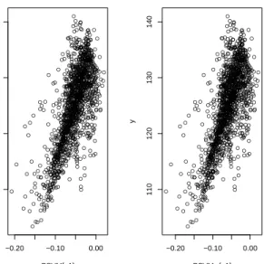
Figure 1: The picture on the left shows the first direction of the PSVM algorithm with the response and the one on the right the first direction of the adaptively weighted PSVM algorithm. ● ● ● ● ● ● ● ● ● ● ● ● ● ● ● ● ● ● ● ● ● ● ● ● ● ● ● ● ● ● ● ● ● ● ● ● ● ● ● ● ● ● ● ● ● ● ● ● ● ● ● ● ● ● ● ● ● ● ● ● ● ● ● ● ● ● ● ● ● ● ● ● ● ● ● ● ● ● ● ● ● ● ● ● ● ● ● ● ● ● ● ● ● ● ● ● ● ● ● ● ● ● ● ● ● ● ● ● ● ● ● ● ● ● ● ● ● ● ● ● ● ● ● ● ● ● ● ● ● ● ● ● ● ● ● ● ● ● ● ● ● ● ● ● ● ● ● ● ● ● ● ● ● ● ● ● ● ● ● ● ● ● ● ● ● ● ● ● ● ● ● ● ● ● ● ● ● ● ● ● ● ● ● ● ● ● ● ● ● ● ● ● ● ● ● ● ● ● ● ● ● ● ● ● ● ● ● ● ● ● ● ● ● ● ● ● ● ● ● ● ● ● ● ● ● ● ● ● ● ● ● ● ● ● ● ● ● ● ● ● ● ● ● ● ● ● ● ● ● ● ● ● ● ● ● ● ● ● ● ● ● ● ● ● ● ● ● ● ● ● ● ● ● ● ● ● ● ● ● ● ● ● ● ● ● ● ● ● ● ● ● ● ● ● ● ● ● ● ● ● ● ● ● ● ● ● ● ● ● ● ● ● ● ● ● ● ● ● ● ● ● ● ● ● ● ● ● ● ● ● ● ● ● ● ● ● ● ● ● ● ● ● ● ● ● ● ● ● ● ● ● ● ● ● ● ● ● ● ● ● ● ● ● ● ● ● ● ● ● ● ● ● ● ● ● ● ● ● ● ● ● ● ● ● ● ● ● ● ● ● ● ● ● ● ● ● ● ● ● ● ● ● ● ● ● ● ● ● ● ● ● ● ● ● ● ● ● ● ● ● ● ● ● ● ● ● ● ● ● ● ● ● ● ● ● ● ● ● ● ● ● ● ● ● ● ● ● ● ● ● ● ● ● ● ● ● ● ● ● ● ● ● ● ● ● ● ● ● ● ● ● ● ● ● ● ● ● ● ● ● ● ● ● ● ● ● ● ● ● ● ● ● ● ● ● ● ● ● ● ● ● ● ● ● ● ● ● ● ● ● ● ● ● ● ● ● ● ● ● ● ● ● ● ● ● ● ● ● ● ● ● ● ● ● ● ● ● ● ● ● ● ● ● ● ● ● ● ● ● ● ● ● ● ● ● ● ● ● ● ● ● ● ● ● ● ● ● ● ● ● ● ● ● ● ● ● ● ● ● ● ● ● ● ● ● ● ● ● ● ● ● ● ● ● ● ● ● ● ● ● ● ● ● ● ● ● ● ● ● ● ● ● ● ● ● ● ● ● ● ● ● ● ● ● ● ● ● ● ● ● ● ● ● ● ● ● ● ● ● ● ● ● ● ● ● ● ● ● ● ● ● ● ● ● ● ● ● ● ● ● ● ● ● ● ● ● ● ● ● ● ● ● ● ● ● ● ● ● ● ● ● ● ● ● ● ● ● ● ● ● ● ● ● ● ● ● ● ● ● ● ● ● ● ● ● ● ● ● ● ● ● ● ● ● ● ● ● ● ● ● ● ● ● ● ● ● ● ● ● ● ● ● ● ● ● ● ● ● ● ● ● ● ● ● ● ● ● ● ● ● ● ● ● ● ● ● ● ● ● ● ● ● ● ● ● ● ● ● ● ● ● ● ● ● ● ● ● ● ● ● ● ● ● ● ● ● ● ● ● ● ● ● ● ● ● ● ● ● ● ● ● ● ● ● ● ● ● ● ● ● ● ● ● ● ● ● ● ● ● ● ● ● ● ● ● ● ● ● ● ● ● ● ● ● ● ● ● ● ● ● ● ● ● ● ● ● ● ● ● ● ● ● ● ● ● ● ● ● ● ● ● ● ● ● ● ● ● ● ● ● ● ● ● ● ● ● ● ● ● ● ● ● ● ● ● ● ● ● ● ● ● ● ● ● ● ● ● ● ● ● ● ● ● ● ● ● ● ● ● ● ● ● ● ● ● ● ● ● ● ● ● ● ● ● ● ● ● ● ● ● ● ● ● ● ● ● ● ● ● ● ● ● ● ● ● ● ● ● ● ● ● ● ● ● ● ● ● ● ● ● ● ● ● ● ● ● ● ● ● ● ● ● ● ● ● ● ● ● ● ● ● ● ● ● ● ● ● ● ● ● ● ● ● ● ● ● ● ● ● ● ● ● ● ● ● ● ● ● ● ● ● ● ● ● ● ● ● ● ● ● ● ● ● ● ● ● ● ● ● ● ● ● ● ● ● ● ● ● ● ● ● ● ● ● ● ● ● ● ● ● ● ● ● ● ● ● ● ● ● ● ● ● ● ● ● ● ● ● ● ● ● ● ● ● ● ● ● ● ● ● ● ● ● ● ● ● ● ● ● ● ● ● ● ● ● ● ● ● ● ● ● ● ● ● ● ● ● ● ● ● ● ● ● ● ● ● ● ● ● ● ● ● ● ● ● ● ● ● ● ● ● ● ● ● ● ● ● ● ● ● ● ● ● ● ● ● ● ● ● ● ● ● ● ● ● ● ● ● ● ● ● ● ● ● ● ● ● ● ● ● ● ● ● ● ● ● ● ● ● ● ● ● ● ● ● ● ● ● ● ● ● ● ● ● ● ● ● ● ● ● ● ● ● ● ● ● ● ● ● ● ● ● ● ● ● ● ● ● ● ● ● ● ● ● ● ● ● ● ● ● ● ● ● ● ● ● ● ● ● ● ● ● ● ● ● ● ● ● ● ● ● ● ● ● ● ● ● ● ● ● ● ● ● ● ● ● ● ● ● ● ● ● ● ● ● ● ● ● ● ● ● ● ● ● ● ● ● ● ● ● ● ● ● ● ● ● ● ● ● ● ● ● ● ● ● ● ● ● ● ● ● ● ● ● ● ● ● ● ● ● ● ● ● ● ● ● ● ● ● ● ● ● ● ● ● ● ● ● ● ● ● ● ● ● ● ● ● ● ● ● ● ● ● ● ● ● ● ● ● ● ● ● ● ● ● ● ● ● ● ● ● ● ● ● ● ● ● ● ● ● ● ● ● ● ● ● ● ● ● ● ● ● ● ● ● ● ● ● ● ● ● ● ● ● ● ● ● ● ● ● ● ● ● ● ● ● ● ● ● ● ● ● ● ● ● ● ● ● ● ● ● ● ● ● ● ● ● ● ● ● ● ● ● ● ● ● ● ● ● ● ● ● ● ● ● ● ● ● ● ● ● ● ● ● ● ● ● ● ● ● ● ● ● ● ● ● ● ● ● ● ● ● ● ● ● ● ● ● ● ● ● ● ● ● ● ● ● ● ● ● ● ● ● −0.20 −0.10 0.00 110 120 130 140 L2[, 1] y ● ● ● ● ● ● ● ● ● ● ● ● ● ● ● ● ● ● ● ● ● ● ● ● ● ● ● ● ● ● ● ● ● ● ● ● ● ● ● ● ● ● ● ● ● ● ● ● ● ● ● ● ● ● ● ● ● ● ● ● ● ● ● ● ● ● ● ● ● ● ● ● ● ● ● ● ● ● ● ● ● ● ● ● ● ● ● ● ● ● ● ● ● ● ● ● ● ● ● ● ● ● ● ● ● ● ● ● ● ● ● ● ● ● ● ● ● ● ● ● ● ● ● ● ● ● ● ● ● ● ● ● ● ● ● ● ● ● ● ● ● ● ● ● ● ● ● ● ● ● ● ● ● ● ● ● ● ● ● ● ● ● ● ● ● ● ● ● ● ● ● ● ● ● ● ● ● ● ● ● ● ● ● ● ● ● ● ● ● ● ● ● ● ● ● ● ● ● ● ● ● ● ● ● ● ● ● ● ● ● ● ● ● ● ● ● ● ● ● ● ● ● ● ● ● ● ● ● ● ● ● ● ● ● ● ● ● ● ● ● ● ● ● ● ● ● ● ● ● ● ● ● ● ● ● ● ● ● ● ● ● ● ● ● ● ● ● ● ● ● ● ● ● ● ● ● ● ● ● ● ● ● ● ● ● ● ● ● ● ● ● ● ● ● ● ● ● ● ● ● ● ● ● ● ● ● ● ● ● ● ● ● ● ● ● ● ● ● ● ● ● ● ● ● ● ● ● ● ● ● ● ● ● ● ● ● ● ● ● ● ● ● ● ● ● ● ● ● ● ● ● ● ● ● ● ● ● ● ● ● ● ● ● ● ● ● ● ● ● ● ● ● ● ● ● ● ● ● ● ● ● ● ● ● ● ● ● ● ● ● ● ● ● ● ● ● ● ● ● ● ● ● ● ● ● ● ● ● ● ● ● ● ● ● ● ● ● ● ● ● ● ● ● ● ● ● ● ● ● ● ● ● ● ● ● ● ● ● ● ● ● ● ● ● ● ● ● ● ● ● ● ● ● ● ● ● ● ● ● ● ● ● ● ● ● ● ● ● ● ● ● ● ● ● ● ● ● ● ● ● ● ● ● ● ● ● ● ● ● ● ● ● ● ● ● ● ● ● ● ● ● ● ● ● ● ● ● ● ● ● ● ● ● ● ● ● ● ● ● ● ● ● ● ● ● ● ● ● ● ● ● ● ● ● ● ● ● ● ● ● ● ● ● ● ● ● ● ● ● ● ● ● ● ● ● ● ● ● ● ● ● ● ● ● ● ● ● ● ● ● ● ● ● ● ● ● ● ● ● ● ● ● ● ● ● ● ● ● ● ● ● ● ● ● ● ● ● ● ● ● ● ● ● ● ● ● ● ● ● ● ● ● ● ● ● ● ● ● ● ● ● ● ● ● ● ● ● ● ● ● ● ● ● ● ● ● ● ● ● ● ● ● ● ● ● ● ● ● ● ● ● ● ● ● ● ● ● ● ● ● ● ● ● ● ● ● ● ● ● ● ● ● ● ● ● ● ● ● ● ● ● ● ● ● ● ● ● ● ● ● ● ● ● ● ● ● ● ● ● ● ● ● ● ● ● ● ● ● ● ● ● ● ● ● ● ● ● ● ● ● ● ● ● ● ● ● ● ● ● ● ● ● ● ● ● ● ● ● ● ● ● ● ● ● ● ● ● ● ● ● ● ● ● ● ● ● ● ● ● ● ● ● ● ● ● ● ● ● ● ● ● ● ● ● ● ● ● ● ● ● ● ● ● ● ● ● ● ● ● ● ● ● ● ● ● ● ● ● ● ● ● ● ● ● ● ● ● ● ● ● ● ● ● ● ● ● ● ● ● ● ● ● ● ● ● ● ● ● ● ● ● ● ● ● ● ● ● ● ● ● ● ● ● ● ● ● ● ● ● ● ● ● ● ● ● ● ● ● ● ● ● ● ● ● ● ● ● ● ● ● ● ● ● ● ● ● ● ● ● ● ● ● ● ● ● ● ● ● ● ● ● ● ● ● ● ● ● ● ● ● ● ● ● ● ● ● ● ● ● ● ● ● ● ● ● ● ● ● ● ● ● ● ● ● ● ● ● ● ● ● ● ● ● ● ● ● ● ● ● ● ● ● ● ● ● ● ● ● ● ● ● ● ● ● ● ● ● ● ● ● ● ● ● ● ● ● ● ● ● ● ● ● ● ● ● ● ● ● ● ● ● ● ● ● ● ● ● ● ● ● ● ● ● ● ● ● ● ● ● ● ● ● ● ● ● ● ● ● ● ● ● ● ● ● ● ● ● ● ● ● ● ● ● ● ● ● ● ● ● ● ● ● ● ● ● ● ● ● ● ● ● ● ● ● ● ● ● ● ● ● ● ● ● ● ● ● ● ● ● ● ● ● ● ● ● ● ● ● ● ● ● ● ● ● ● ● ● ● ● ● ● ● ● ● ● ● ● ● ● ● ● ● ● ● ● ● ● ● ● ● ● ● ● ● ● ● ● ● ● ● ● ● ● ● ● ● ● ● ● ● ● ● ● ● ● ● ● ● ● ● ● ● ● ● ● ● ● ● ● ● ● ● ● ● ● ● ● ● ● ● ● ● ● ● ● ● ● ● ● ● ● ● ● ● ● ● ● ● ● ● ● ● ● ● ● ● ● ● ● ● ● ● ● ● ● ● ● ● ● ● ● ● ● ● ● ● ● ● ● ● ● ● ● ● ● ● ● ● ● ● ● ● ● ● ● ● ● ● ● ● ● ● ● ● ● ● ● ● ● ● ● ● ● ● ● ● ● ● ● ● ● ● ● ● ● ● ● ● ● ● ● ● ● ● ● ● ● ● ● ● ● ● ● ● ● ● ● ● ● ● ● ● ● ● ● ● ● ● ● ● ● ● ● ● ● ● ● ● ● ● ● ● ● ● ● ● ● ● ● ● ● ● ● ● ● ● ● ● ● ● ● ● ● ● ● ● ● ● ● ● ● ● ● ● ● ● ● ● ● ● ● ● ● ● ● ● ● ● ● ● ● ● ● ● ● ● ● ● ● ● ● ● ● ● ● ● ● ● ● ● ● ● ● ● ● ● ● ● ● ● ● ● ● ● ● ● ● ● ● ● ● ● ● ● ● ● ● ● ● ● ● ● ● ● ● ● ● ● ● ● ● ● ● ● ● ● ● ● ● ● ● ● ● ● ● ● ● ● ● ● ● ● ● ● ● ● ● ● ● ● ● ● ● ● ● ● ● ● ● ● ● ● ● ● ● ● ● ● ● ● ● ● ● ● ● ● ● ● ● ● ● ● ● ● ● ● ● ● ● ● ● ● ● ● ● ● ● ● ● ● ● ● ● ● ● ● ● ● ● ● ● ● ● ● ● ● ● ● ● ● ● ● ● −0.20 −0.10 0.00 110 120 130 140 L2w[, 1] y

Figure 2: The picture on the left shows the first direction of the PL2SVM algorithm with the response and the one on the right the first direction of the adaptively weighted PL2SVM algorithm.

slices. All algorithms identify similar directions as is shown in Figure 1 and Figure 2. (If one looks carefully the two Figures they may be able to see that the weighted version have slightly smaller variability). The similarity of the results makes sense as it seems that there are no extreme outliers in the dataset. To demonstrate the effectiveness of the reweighted version we added 3 extreme outliers to our datasets. To create this scenario we randomly chose three out of the 10 smallest responses and change the response so that it becomes the largest. Then we measure the distance between the estimate we get when there are outliers from the true estimate we had without the outliers (essentially assuming that without the outliers we have some type of “oracle” answer). We used the Frobenius norm as with our simulations in the previous section and the results after 50 iterations are summarized in the Table 2 where we can see that there is slightly smaller distance for the adaptively weighted algorithms compared to the respective un-weighted algorithms.

7

Discussion

In this paper we present an adaptively weighted method to robustify SVM-based suffi-cient dimension reduction algorithms at the present of outliers. We apply a reweight-ing method based to the idea of Wu and Liu (2013) on the PSVM and PL2SVM algorithms proposed in Li, Artemiou and Li (2011) and Artemiou and Dong (2016) respectively. For the adaptively weighted PL2SVM we present some asymptotic re-sults while the rere-sults for the adaptively weighted PSVM are similar to the ones presented by Shin et al (2017) and therefore are omitted. We also omitted the dis-cussion of an order determination tests as either of the algorithms presented in Li, Artemiou and Li (2011) and Artemiou and Dong (2016) for order determination can be applied here with similar results.

We didn’t discuss also the nonlinear feature extraction case of the adaptively weighted algorithms. Although one can show the theoretical developments of Li, Artemiou and Li (2011) and Artemiou and Dong (2016) to extend in the nonlinear adaptively weighted algorithms, it is not clear in the SDR framework how to calculate the weights. This has to do with the estimation procedure which calculates the sufficient predictors instead of the nonlinear hyperplane between the two classes. We believe that further investigation is needed in this case.

In the SDR literature there are some efforts to robustify inverse-moment-based dimension reduction techniques (see for example Dong et al - 2015) but to the best of our knowledge this is the first effort to robustify SVM-based sufficient dimension

reduction techniques. There is scope for further investigation of these results as well as further investigation of robust algorithms in the SVM-based framework. For example, in this work we investigate what happens when we apply the weights once after running the initial algorithm with no weights. One natural extension is to apply an iterative process where the weights calculated at step i will be used to robustify the algorithm at stepi+1. Although computationally this seems like a trivial extension, the theoretical developments will be non-trivial to develop. Furthermore, the algorithms we propose in this work reweight only points that are outliers with respect to other points in their class, that is, they are misclassified points. If an outlier is correctly classified, since it does not affect the solution then there is no reweighting. An algorithm to investigate how to robustify the original algorithms against all outliers in the dataset will, also, be interesting to explore. Finally, there is scope to investigate whether one can robustify inverse-moment-based dimension reduction techniques (like SIR (Li 1991)) by adaptively reweighting them.

References

1. Artemiou, A. and Dong, Y. (2016). Sufficient dimension reduction via principal Lq support vector machine. Electronic Journal of Statistics,10, 783–805. 2. Artemiou, A. and Shu, M. (2014). A cost based reweighed scheme of

princi-pal support vector machine. In Topics in Nonparametric Statistics, Springer Proceedings in Mathematics & Statistics,74, 1–12.

3. Bura, E. and Pfeiffer, R. (2008). On the distribution of the left singular vectors of a random matrix and its applications. Statistics and Probability Letters,78, 2275–2280.

4. Cook, R. D. (1998a). Regression Graphics: Ideas for Studying Regressions through Graphics. New York: Wiley.

5. Cook, R. D. (1998b). Principal Hessian directions revisited (with discussion). Journal of the American Statistical Association,93, 84–100.

6. Cook, R. D. and Weisberg, S. (1991). Discussion of “Sliced inverse regression for dimension reduction”. Journal of the American Statistical Association. 86, 316–342.

7. Dong, Y., Yu, Z. and Zhu, L. (2015). Robust inverse regression for dimension reduction. Journal of Multivariate Analysis,134, 71–81.

8. Li, B., Artemiou, A. and Li, L. (2011). Principal support vector machine for linear and nonlinear sufficient dimension reduction. The Annals of Statistics, 39, 3182–3210

9. Li, B. and Wang, S. (2007). On directional regression for dimension reduction. Journal of the American Statistical Association,102, 997–1008.

10. Li, B., Zha, H., and Chiaromonte, F. (2005). Contour regression: a general approach to dimension reduction. The Annals of Statistics,33, 1580–1616. 11. Li, K. C. (1991). Sliced inverse regression for dimension reduction (with

discus-sion). Journal of the American Statistical Association,86, 316–342.

12. Li, K. C. (1992). On principal Hessian directions for data visualization and dimension reduction: another application of Stein’s Lemma. Journal of the American Statistical Association,87, 1025–1039.

13. Lin, Y., Lee, Y. and Wahba, G. (2002). Support vector machines for classifica-tion in nonstandard situaclassifica-tions. Machine Learning,46, 191-202.

14. Shin, S. J., Wu, Y., Zhang, H. H. and Liu, Y. (2014). Probability-enhanced sufficient dimension reduction for binary classification. Biometrics, 70, 546– 555.

15. Shin, S. J., Wu, Y., Zhang, H. H. and Liu, Y. (2017). Principal weighted sup-port vector machines for sufficient dimension reduction in binary classification. Biometrika,104, 67–81.

16. Wu, Y and Liu, Y. (2013). Adaptively weighted large margin classifiers. Journal of Computational and Graphical Statistics,22, 416–432