Benchmarking SQL on MapReduce systems using large
astronomy databases
Amin Mesmoudi, Mohand-Sa¨ıd Hacid, Farouk Toumani
To cite this version:
Amin Mesmoudi, Mohand-Sa¨ıd Hacid, Farouk Toumani. Benchmarking SQL on MapReduce
systems using large astronomy databases. Distributed and Parallel Databases, Springer, 2015,
<
10.1007/s10619-014-7172-8
>
.
<
hal-01221665
>
HAL Id: hal-01221665
https://hal.inria.fr/hal-01221665
Submitted on 28 Oct 2015
HAL
is a multi-disciplinary open access
archive for the deposit and dissemination of
sci-entific research documents, whether they are
pub-lished or not.
The documents may come from
teaching and research institutions in France or
abroad, or from public or private research centers.
L’archive ouverte pluridisciplinaire
HAL
, est
destin´
ee au d´
epˆ
ot et `
a la diffusion de documents
scientifiques de niveau recherche, publi´
es ou non,
´
emanant des ´
etablissements d’enseignement et de
recherche fran¸cais ou ´
etrangers, des laboratoires
publics ou priv´
es.
(will be inserted by the editor)
Benchmarking SQL On MapReduce systems using
large astronomy databases
Amin Mesmoudi · Mohand-Sa¨ıd Hacid · Farouk Toumani
Received: date / Accepted: date
Abstract In the era of bigdata, with a massive set of digital information of un-precedented volumes being collected and/or produced in several application do-mains, it becomes more and more difficult to manage and query large data reposi-tories. In the framework of the PetaSky project (http://com.isima.fr/Petasky), we focus on the problem of managing scientific data in the field of cosmology. The data we consider are those of the LSST project (http://www.lsst.org/). The overall size of the database that will be produced is expected to exceed 60 PB [28]. In order to evaluate the performances of existing SQL On MapReduce data management systems, we conducted extensive experiments by using data and queries from the area of cosmology. The goal of this work is to report on the ability of such systems to support large scale declarative queries. We mainly investigated the impact of data partitioning, indexing and compression on query execution performances.
1 Introduction and Context
In the age of bigdata, a massive set of digital information of unprecedented vol-umes are being collected and/or produced in several application domains, making it increasingly difficult to manage and query large data repositories. While tradi-tional database management systems (DBMS) have gain their reputation thanks to their support of SQL, a declarative, simple and efficient language, they turn out to be less effective when it comes to manage very large data repositories [32]. As a consequence, there has been recently an increasing trend towards using ad hoc This work is partially supported by Centre National de la Recherche Scientifique-CNRS, under the project Petasky-Mastodons (http://com.isima.fr/Petasky)
A. Mesmoudi and M-S Hacid Universit´e de Lyon, CNRS
Universit´e Lyon 1, LIRIS, UMR5205, F-69622, France E-mail:{amin.mesmoudi,mshacid}@liris.cnrs.fr F. Toumani
Blaise Pascal University, CNRS
tools instead of DBMS in several data management applications. Being aware of this fact, database research and development community and DBMS vendors [14] have been conducting intensive efforts towards the development of advanced tools intended to be embodied in the advanced generations of DBMS products in order to support big data management. Several application domains, like social net-works [31], astronomy [28] and Web [13] express a clear need for new approaches for data management and analysis. For instance, Google provided the basis of MapReduce [13], a new computing paradigm designed to enable efficient process-ing of huge amounts of data on a multitude of machines in a cluster.MapReduce provides a simple programming framework that enables harnessing the power of very large data centers, while hiding low level programming details related to par-allelization, fault tolerance, and load balancing. When using such a framework, users have only to specify two functions, namely Map and Reduce, and the sys-tem (e.g., Hadoop-http://hadoop.apache.org/) schedules1 a parallel execution of these functions over the available nodes of a given cluster. The MapReduce ap-proach has been proven particularly efficient to implement one pass algorithms (i.e., algorithms that require only a single scan of data) [19].
As part of the Petasky project (http://com.isima.fr/Petasky), the work pre-sented in this paper addresses several challenges related to performance evalu-ation of MapReduce based systems in the context of a specific application re-lated to analysis and management of scientific data in the field of cosmology. Petasky uses as application context, i.e., data, queries and system requirements, LSST (Large Synoptic Survey Telescope- http://lsst.in2p3.fr/projet-LSST.html), a project which targets the construction of a telescope of a new generation with a light-gathering power among the largest in the world. Data management and analysis is recognized as one of the most challenging aspects of the LSST [28], as more than 30 TB (TeraBytes) of complex data (3.2 Gigapixel images, uncertain data, multi-scale data) must be processed and stored each night to produce the largest non-proprietary data set in the world. The LSST data management group
(http://www.slac.stanford.edu/) recommends the use of an open Source
sys-tem based on a shared nothing architecture. Two main factors motivated such a recommendation: (i) integration of personalized optimization and adhoc features is facilitated, and (ii) support of declarative queries. Taking into account these recommendations, our main objective was to evaluate the capabilities of some systems to manage LSST data, the expected data volume at the end of the acqui-sition process is 60 PB (PetaBytes), using as infrastructure a cluster of hundreds of commodity servers. We focused our study on MapReduce systems for the following reasons:
– the programming model underlying such approaches enables easy development of scalable parallel applications, even for programmers without experience with distributed systems (this because the system hides the details of parallelization, fault-tolerance, locality optimization, and load balancing),
– a large variety of problems can be expressed as MapReduce computations,
– a MapReduce framework is able to scale to large clusters with thousands of nodes.
Previous works (e.g.[25]) on benchmarking have stressed the technological su-periority of parallel DBMS compared to Hadoop, which is mainly due to a lack of
sophisticated optimization mechanisms (e.g., compression, buffering, indexing) in Hadoop. Recently, new systems (e.g.,HadoopDB[9, 12],Hive[33]) have been pro-posed to strenghten MapReduce technologies with a declarative query language, in order to facilitate the expression of repeated complex tasks, as well as with sophisticated optimisation techniques. These systems are based on the idea of generating, from an SQL(-Like) query, a set of MapReduce jobs whose execution and resources management will be supported by a MapReduce framework. In this paper, we specifically report on the capability of two such systems, namelyHive and HadoopDB, to accommodate LSST data management requirements.
To achieve our goal, we designed and set up a benchmark to evaluate the per-formance of SQL On MapReduce data management systems. We used data sets and queries from the area of cosmology, provided by the LSST project. We ex-tensively investigated two systems as use cases:Hive, an HDFS based system and HadoopDB, a Hadoop/PostgreSQL based system. In contrast to existing bench-marks (e.g., TeraSort [4], Pavlo et al. [25], Intel HiBench [17]), our benchmark considers real structured data and real queries which makes evaluation of the sys-tems relevant. We also defined additional queries (e.g., distance join,...) which can be very useful to evaluate other kinds of complex computations over structured data. In this context, we conducted extensive experiments to evaluate the two SQL On MapReduce systems to manage (e.g., storage, loading) LSST data on one hand and their capabilities (i.e., indexing, compression, buffering, and par-titioning) to optimize some categories of queries on the other hand. In contrast to existing experiments we do not consider only execution time but also loading time. We investigated different configurations obtained by varying the values of the parameters we consider:
– Infrastructure: we used different sizes for the clusters, one with 25nodes and another with50nodes.
– Data:we use different datasets with sizes of 250 GB,500 GB,1 TBand 2 TB.
– Partitioning:we used two partitioning schemas and we compared execution time for both schemas.
– Indexing:we run our queries on both indexed and non-indexed data. ForHive, we used different attributes as indexes.
– Selectivity: we considered queries with different selectivities (i.e., the number of records that satisfy the query).
Additional information and technical details about this benchmark are available at: http://com.isima.fr/Petasky/hive-vs-hadoopdb.
The rest of this paper is organized as follows: In Section 2, we briefly review basic notions related toMapReduce based systems and we highlight the need for a new benchmark for SQL on MapReduce solutions. In Section 3, we present the main features of the datasets used in our experiments. In Section 4, we describe the experiments and we discuss the outcomes in Section 5. We conclude in Section 6.
2 Background and Related Work
In this section, we review basic notions underlying aMapReduceframework and its extensions to support SQL queries and we discuss existingMapReducebenchmarks.
We start by introducing a running example that will be used through the paper to illustrate the investigated issues.
2.1 A running example
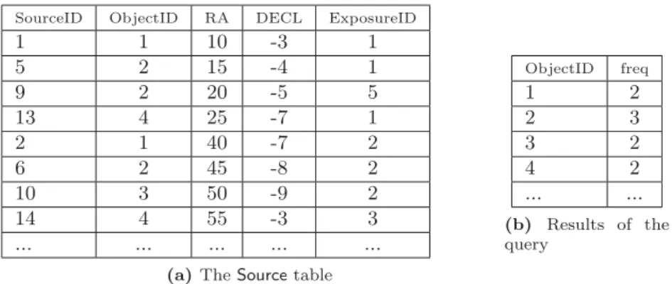
We use an example from the field of astronomical observations [28]. We consider a simple relational database schema which includes two tables. The first table, called Source, is used to store detected astronomical objects extracted from acquired images. This table includes attributes that represent the ID of the observation (SourceID), theIDof the detected object (ObjectID), the world coordinates: Right Ascension (RA) and Declination (Decl) and science exposure ID (ExposureID). As query, we use a slightly adapted query2 from the LSST workload. This query, given below, returns appearance frequency of detected astronomical objects in the database:
SELECT ObjectID,
count(SourceID) as freq (q)
FROM Source GROUP BY objectID
Table1ashows some sample data of the relationSourcewhile table1bshows an extract of the expected results when the previous query is executed over table1a.
SourceID ObjectID RA DECL ExposureID
1 1 10 -3 1 5 2 15 -4 1 9 2 20 -5 5 13 4 25 -7 1 2 1 40 -7 2 6 2 45 -8 2 10 3 50 -9 2 14 4 55 -3 3 ... ... ... ... ...
(a)TheSourcetable
ObjectID freq 1 2 2 3 3 2 4 2 ... ... (b) Results of the query
Table 1:Examples of content of the tableSourceand the result returned by the query (q)
2.2 MapReduce
MapReduceis a new programming model that is intended to be used to facilitate the development of scalable parallel computations on large server clusters [13]. A MapReduce framework enables to perform computations through two simple programming primitives:MapandReducefunctions. AMapfunction takes as input a data set in form of a set of key/value pairs and, for every pair< k, v >of the input
returns zero or more intermediate key-value pairs< k;v>. The map outputs are then processed by a reduce function which implements an application specific business logic. A reduce function takes as input a key-list pair < k;list(v) >, where k is an intermediate key and list(v) is the list of all the intermediate values associated with the key k, and returns as final result zero or more key-value pairs< k, v >. Several instantiations of the map and reduce functions can operate simultaneously on different nodes of the cluster. A Map’s intermediate results are stored in the local file system and sorted by the keys. After all the Maptasks are completed, theMapReduceengine notifies theReducetasks (which are also processes that are referred to as Reducers) to start their execution. The Reducerspull the output files from theMap tasks in parallel and merge-sort the files obtained from theMaptasks to combine the key/value pairs into a set of new key/value pairs< k;list(v)>.
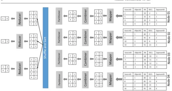
We shall illustrate now aMapReduceprocess using our running example. Fig-ure 1 shows the sequence of data processing steps. First, we assume that data is partitioned over nodes of the cluster. An approach to useMapReduceframework to process our sample query is to defineMap andReducefunctions as follows:
– Map: for each record assigned to aMapper, one generates a (key, value) where key is the value of the attribute ObjectID and the value is 1.
– Reduce: for each received input < Key, list < V alue >>, one applies the addition onlist < value >,i.e.,list < f req >.
The system starts by reading each record in the database and generates a set of
< ObjectID,1>by applying theMapfunction. Combiners perform a grouping on sameObjectIDs on< ObjectID, f req > leading to< ObjectID, list < f req >>. Partitioners are then used to choose aReducerrecipient. By default, a hash function is used. In the Shuffleand Sort phases, a transfer of local key,list < value >to Reducers is done. Finally, each Reducer applies the Reduce function on received pairs< key, List < value >>.
There are several implementations of the MapReduce framework. The most popular one is Hadoop. Indeed, Hadoop uses HDFS [29] to store and partition data on nodes of a cluster. Data is partitioned in chunks (by default each chunk has a size of 64 MB). Each Map task is assigned to a chunk.Hadoop also offers default functions that can be used as combiners and partitionners. These functions could easily be replaced by other functions defined by the user. Other implementa-tions ofMapReduce,e.g., Themis and SailFish, exist. Themis [27] is aMapReduce implementation designed for small clusters where the probability of node failure is much lower. It achieves high efficiency by eliminating task-level fault tolerance. Compared to Hadoop, Sailfish [26] changes the transport layer between Mappers andReducers. The authors in [26] tried to improve the disk subsystem performance for large scaleMapReducecomputations by aggregating intermediate data.
A new version ofHadoop, called YARN [35], enhances the power of aHadoop framework by improving cluster utilization and providing support for workloads other than MapReduce. Tez [8] is another in-progress project which allows to speed up data processing across both small-scale, low-latency and large-scale, high-throughput workloads. This is achieved by eliminating unnecessary tasks, synchronization barriers, and reads from and write to HDFS. Other implementa-tions ofMapReduceon specialized hardware are proposed. For example, Mars [15] is aMapReduceframework on graphics processors.
Fig. 1:Illustration of sample query processing using MapReduce
2.3 Relational operations on top of MapReduce
A lot of recent research work has been devoted to the implementation and op-timization of relational operations using theMapReduce computation model. For example, Select-P roject queries have been initially implemented using a single Map function. However, a drawback of such a solution comes from a need to achieve a full scan of all the data for each query, and this is a very costly task. To overcome such a limitation, main optimization techniques consist in the use of indexing and data compression. Instead of transferring all key/values pairs of chunks to Mappers, a filtering phase is applied to identify only relevant data to be transferred. With respect to data compression, a major proposal lies in the notion of RCFile [16]. In this case, less data is transferred from disk to RAM. Besides
Select-P roject, implementations of other relational operators have been proposed in the literature. Implementation ofGROU P BY (see figure 1) queries is discussed in section 2.2 whileSorting(ORDERBY) will be discussed in section 4.6.4.
The join operation is very expensive if one considers its implementation using the MapReduce model [10]. Indeed, in the case of non constrained inputs, many records that do not contribute to the final results will be transferred toReducers. Some sophisticated implementations have been proposed to overcome the limi-tations of the naive approach. For example, Afrati et al. propose to control the number of Reducersto take advantage of the available resources for simple equi-join [10] and Multi-way equi-equi-join [11].
Another relevant (non classical) operator for the LSST queries is similarity join. Indeed, this operation allows to group together records that have a distance (computed from some attributes) less or equal than a given threshold. Several approaches (e.g.,[30, 24, 23, 20, 18]) have been proposed to compute some kinds of similarity joins using the MapReduce model. For example, if one wants to group
together observations with a distance less than 15 degrees, one can specify the following query:
SELECT S1.objectID, S2.objectID FROM Source as S1,Source as S2 WHERE
AngDist(S1.DECL,S2.DECL,S1.RA,S2.RA) <15
WhereAngDistis the angular distance3 between two observations (sources),i.e.: AngDist(S1.DECL,S2.DECL,S1.RA,S2.RA) =
sin(S1.DECL)sin(S2.DECL)
+ cos(S1.DECL)cos(S2.DECL)cos(S1.RA-S2.RA)
The attributes S.Ra and S.DECL record the right ascension and declination, in degrees, related to a given observationS.
2.4 SQL on MapReduce
Several frameworks have been proposed to extend MapReduce models with SQL capabilities. We distinguish between two types of systems. In the first type, the implementation of theMapReduceframework does not change. For instance,Hive proposes to transform SQL queries into a set ofMapReduceJobs.HadoopDB fol-lows the same principle but it uses an existing RDBMS to store the data in each worker, instead of the HDFS which is used byHive. This allows to exploit indexing, buffering and compression capabilities offered by DBMSs.
The second type of systems requires a substantial change in the MapReduce framework. Essentially, this type of tools is based on the idea of loading all the data into the memory. For example, Shark [36] is based on the Spark[5] framework. Impala [2] is a Hive-compatible SQL engine with its own MPP (Massively Parallel Processing) execution engine. Stinger [6] is another in-progress project based on Tez. Presto [3] is an open source distributed SQL developed by Facebook for interactive queries. Other tools are proposed such as BigSQL [1] which is based onHadoopon one hand and PostgresQL on the other hand.
2.5 MapReduce benchmark
Several benchmarks forMapReduce frameworks exist. Historically, the first one is TeraSort[4] which is devoted to testMapReduceimplementations using a large scale sort application.Hadoopoffers a set of tools to benchmark several implementations of MapReduce frameworks. For example, TestDFSIO[7] is a tool devoted to test I/O capabilities of DFS systems used inMapReduceframeworks. Pavlo etal.[25] proposed a customized benchmark tailored for search engines where a comparison between Hadoop and two parallel DBMS (Vertica and DBMS-X) was proposed. The conclusion of that work highlights the inability of existing implementations (the version of 0.19 ofHadoop has been used ) of theMapReduce model to effec-tively process data. Three tasks have been tested: selection, aggregation and join.
The maximum number of attributes of the tables used in the experiments is nine (9) and the considered join query involves two tables. Authors stressed the tech-nological superiority of parallel DBMS compared to Hadoop, which is mainly due to a lack of sophisticated optimization mechanisms (e.g., compression, buffering, indexing) in Hadoop.
In [9] the same benchmark was used. Authors compared Parallel DBMS, HadoopDB and Hadoop (as an implementation of MapReduce framework). As con-clusion, authors noticed that a hybrid system (i.e., HadoopDB) MapReduce and DBMS could achieve performances of parallel DBMSs. Authors in [12] extended experiments in [9] by comparing Hadapt (commercial version of HadoopDB), Hive and parallel DBMSs. We believe that this comparison is not complete. Indeed, au-thors tried to highlight the advantages of Hadapt compared to Hive and parallel DBMS without considering all cases.
Since then, several extensions have been proposed to optimize the performance ofMapReduceprograms. We review in the sequel the impact of existing techniques on performances. We also explain in details when one of the two tools (Hive, HadoopDB) outperforms the other.
Intel Hibench [17] suite contains nine (9) workloads, including micro bench-marks, HDFS benchbench-marks, web search benchbench-marks, machine learning benchbench-marks, and data analytics benchmarks. Intel Hibench includes a dataset which is used in Pavlo et al. [25] for analytic tasks. In this work, the authors were interested in measuring resources consumption (e.g., RAM, DISK, CPU) for each execu-tion step within aMapReduce program. BigDataBench [37] is a benchmark suite that proposes various datasets and workloads for various applications from in-ternet services domain. The datasets cover Wikipedia Entries, Amazon Movie Reviews, Google Web Graph, Facebook Social Network, E-commerce Transaction Data, ProfSearch Person Resumes, CALDA Data and TPC-DS Web Data. All the considered datasets, but E-commerce transaction data which uses a relational schema, include unstructured or graph data and focus on basic operations (e.g., grep, wordcount, sort) or analytical processing (k-mean, pagerank, ...). We view our benchmark as complementary to existing benchmarks, including Intel Hibench and BigDataBench, for several reasons. First, our benchmark focuses on an appli-cation domain, data management in the field of cosmology, which is not covered by these benchmarks. Datasets and query workloads in this field display some specific features related to the structure of the data, data volumes, complexity of queries (e.g., using specific UDFs) which are not provided by Intel Hibench and Big-DataBench benchmarks. Moreover, both Intel Hibench and BigBig-DataBench target general MapReduce related applications while, in our work, we especially target SQL on MapReduce systems. We are interested in the implementation and the op-timization of SQL operators using MapReduce model. Our datasets and workload allow us to conduct deep analysis on various aspects specifically related to this kind of systems. Indeed, we allow analysis of the behaviour of these systems with respect to selectivity, partitioning, infrastructure and (data volume) scalability. To the best of our knowledge the two benchmarks (i.e., Hibench, BigDataBench) do not allow to investigate in-depth query evaluation and optimization techniques with scalable structured data.
Our benchmark rests on a real case study. We consider structured data from astronomy where a set of SQL queries are already defined. Our experiments target SQL On MapReduce systems. Our objective is to report on the capabilities of
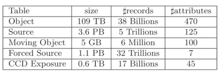
Table size records attributes
Object 109 TB 38 Billions 470
Source 3.6 PB 5 Trillions 125
Moving Object 5 GB 6 Million 100 Forced Source 1.1 PB 32 Trillions 7 CCD Exposure 0.6 TB 17 Billions 45
Table 2:Expected data characteristics
those systems to manage (e.g., storage, loading) LSST data on one hand and their capabilities (i.e., indexing, compression, buffering, and partitioning) to optimize some categories of queries on the other hand. In contrast to existing experiments we do not consider only execution time but also loading time. We consider differ-ent configurations for the differdiffer-ent parameters: Infrastructure, Data, Partitioning, Indexing and Selectivity. Also, our benchmark will serve as a baseline to assess query evaluation and optimization techniques that will be proposed in the context of the Petasky project.
3 Data characteristics
We focus on the issue of data management in the field of cosmology. Data are stored using relational tables where information about exposures, objects and ob-servations can be found. The database is organized in the following four categories (represented as tables):
1. Exposure: describes each exposure, including the start date/time of exposure, the used filter, the position and orientation of the field of view on the sky, and other environmental information.
2. Object: describes attributes of each astrophysical object, including the world coordinates.
3. Source: describes each detected source on each image, including its location (x, y) on the detector, world coordinates (RA, Decl), brightness, size, and shape. 4. Moving Object: describes attributes of moving (solar system) objects, including
orbital elements, brightness, albedo and rotation period.
5. Forced Source: describes measurements computed using source records. Table 2 shows, for some tables, the estimated size of expected data at the end of the observation (which will start in 2020 for a duration of 10 years), the number of attributes as well as the expected final number of tuples. It is worth noting that:(i)the size of the data varies from Gigabytes (e.g., size of the table Moving Object) to a few Petabytes (e.g. size of the tables Source and ForcedSource),(ii) the number of records ranges from few millions (e.g., for the table Moving Object) to trillions (e.g., for the Source table), and (iii) the number of attributes varies from 7, for ForcedSource table, to 450 for the Object table.
In order to evaluate the capacity of existing systems to manage LSST data, the data management group of the LSST project has provided some datasets and a tool to generate other datasets which are compliant with the characteristics of real data. Table3ashows the size of the four datasets PT1.1, PT 1.2, Winter 13 and SDSS
Dataset Size PT 1.1 90 GB PT 1.2 220 GB Winter 13 3 TB SDSS 3 TB (a) Datasets
Table Attributes Records Size
Source 107 162 x 106 118 GB Object 227 4 x 10⁶ 7 GB RefSrcMatch 10 189 x 106 1.7 GB Science Ccd Exposure Metadata 6 41 x 106 16 GB (b)PT 1.2 characteristics
Datasets Source: Source: Object: Object: SourceID ObjectID DECL RA ScienceCcd
Record Size (GB) Record Size (GB) ExposureID
D250GB 325 x 106 236 9 x 10⁶ 14 325 x 106 9 x 10⁶ 325 x 106 162 x 106 84 x 103 D500GB 650 x 106 472 18 x 106 28 650 x 106 18 x 106 650 x 106 162 x 106 84 x 103 D1TB 1.3 x 10⁹ 944 36 x 106 56 1.3 x 10⁹ 36 x 106 1.1 x 10⁹ 162 x 106 84 x 103 D2TB 2.6 x 10⁹ 1888 72 x 106 112 2.6 x 10⁹ 72 x 106 2.3 x 10⁹ 162 x 106 84 x 103
(c)Generated dataset
Table 3:Datasets characteristics
(Sloan Digital Sky Survey, http://www.sdss.org/). Only SDSS dataset is a real dataset collected within the SDSS project. We chose to use for our experiments the dataset PT1.2 whose characteristics are depicted at Table 3b. This dataset contains 22 tables stored as ”CSV” files with a total size of 220 GB. At this stage, we exploited only 4 tables: The Source table that has 107 attributes and contains 180 millions of tuples (for a total size of 139 GB), theObjecttable which has 229 attributes and contains 5 millions of tuples (for a total size of 7 GB), the Science Ccd Exposure Metadatatable which has 6 attributes and contains 41 millions of tuples (for a total size of 16 GB), and theRefSrcMatchtable that has 10 attributes and contains 189 millions of tuples (for a total size of 1.5 GB). To address the scalability issue, we generated4, from PT 1.2 dataset, four (4) new datasets with a total size of 250 GB, 500 GB, 1 TB and 2 TB respectively. New tables are generated only for the tablesSourceandObject. For the other tables, we kept the same records. Table 3c shows the characteristics of the generated data. The four first columns show the number of records and the size of the tablesSource andObjectrespectively. The other columns show the number of distinct values for five attributes of the tableSourceinvolved in our workload.
4 Experiments
4.1 Processing Infrastructure Our experiments are performed over
a distributed system composed of50 nodes. Each node has8 GB of RAM,
300 GB of hard disk storage capacity and 2 cores. Network rate can reach 1
4 generated data comply with the characteristics of real data, we used an algorithm (https:
//dev.lsstcorp.org/trac/wiki/db/Qserv/Duplication) designed by LSST data management group.
GB/s. We set up two clusters of 25 and 50 nodes, respectively. According to hdparm5, the hard disks deliver 113 MB/sec for buffered reads.
Using this distributed architecture, we deployedHadoopDBandHive.
4.2 Hadoop
We used two versions ofHadoop, namely 0.19.1 and 1.1.1., in our experiments. Due to the incompatibility ofHadoopDBwith recent versions ofHadoop,HadoopDBis coupled with Hadoop 0.19.1, whereas Hive is coupled with Hadoop 1.1.1. Both versions run on Java 1.7. We deployed the system by using the configuration mentioned inHadoopDBoriginal paper.6Data inHDFS(Hadoop Distributed File System) is stored using 256 MB data blocks instead of the default 64 MB. Each MapReducejob executor runs with a maximum heap size of 1024 MB.
4.3 Hive
Hiveis based onHadoopopen Source that implements aMapReduce[13] framework. Hive proposes HiveQL, a SQL-like language, to specify analysis tasks. Data is stored using HDFS. From an SQL-like query, Hive enables generating a set of MapReduce tasks and, in addition, it schedules the execution of the generated tasks. In our experiments, we usedHive0.11.
4.4 HadoopDB
HadoopDBis based onHiveand usesHiveQL. Existing DBMS are used to store data in the nodes of the cluster. An execution plan, generated byHive, is processed to push more complex tasks, as for example SQL queries, to nodes in theMapphase. HadoopDBuses an XML file7to store access information to data. In particular, information about chunks and sub-chunks, related to each table, is stored in this file.HadoopDBprocesses queries as follows. First,HadoopDBparses an input query by resorting toHive’s mechanisms. Second, the catalog is parsed and the query is reformulated with respect to chunks and sub chunks information in the catalog. Then, a set ofMapReducejobs are generated together with a predefined execution order. In the Map phase of HadoopDB job, a query is sent to the DBMS and responses are formatted in a<key, value>format. After the execution of theMap and Reduce phases is completed,HadoopDB checks whether there is another job to execute. If any, partial results are stored inHDFS. If there is no additional job to be executed, responses are transferred to the node running aHiveclient. In our work,HadoopDBis coupled with postgresQL in each node of the cluster.
Recently, we conducted experimental studies by using centralized systems [21, 22]: Mysql, PostgreSQL and DBMS-X (a commercialized DBMS). We found that PostgreSQL outperforms Mysql and DBMS-X with respect to LSST data. Also, in [9], the authors noticed that PostgreSQL outperforms Mysql for analytic queries.
5 A tool that gives the average disc speeds (http://en.wikipedia.org/wiki/Hdparm). 6 the same configuration is used in [25], the popularHadoopbenchmark paper.
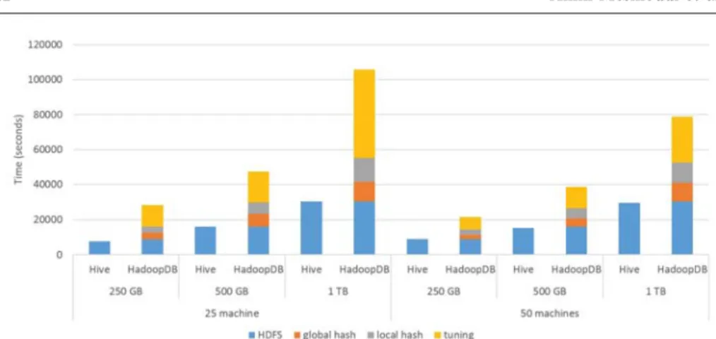
Fig. 2:Data loading: Hive vs. HadoopDB
This is why we believe that HadoopDB coupled with PostgreSQL outperforms HadoopDB coupled with Mysql. Consequently, we choose to discard Mysql and use only PostgreSQL withHadoopDB.
HadoopDB also offers a partitioning tool. This tool is used to minimize the intermediate results of jobs generated byHive. The use of existing DBMS as data storage and access layer allows to exploit existing technologies such as indexing, buffering and compression.
4.5 Data loading and indexing
In this section, we analyze the data loading and indexing techniques of the two selected systems.
4.5.1 Hive
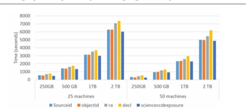
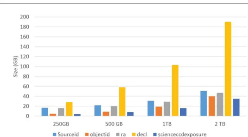
Data loading. The tables are loaded in theHDFSdirectly and stored as text files. Figure 2 shows the time needed to load data in theHDFS for the datasets used in our experiments. One can observe that the time needed for 25 nodes and 50 nodes is the same. The time needed to load datasets for a given cluster (e.g., 50 machines) is linear compared to the size of the dataset. If we have 2X of data8 we need in average 2X of time9 to load data. Indeed, input operations (i.e., reading data from local hard disks) induce the most important part of the loading time. Data indexing. Hive supports only simple indexes with a single attribute. To deal with our query workload, we created 5 indexes: SourceID, ObjectID, RA, DECL and ScienceCCDExposureId. The time overhead due to creation of indexes is shown on figure 3, whereas the space overhead (i.e., size of the indexes) is shown on figure 4. For each attribute, a set of<key, set ofHDFS addresses> is stored in the HDFS. This structure is used to filter relevant records for a given query.
8 In the rest of paper, we use the notation nX of data to denote the size n times. 9 In the rest of paper, we use the notation nX of time to denote the time n times.
Fig. 3:Hive: Data indexing
The creation of the index is linear compared to the size of data. RA and DECL are both of typedouble, whereas SourceID, ObjectID and ScienceCCDExposure are of type BigInt. The Indexing of SourceID requires more time compared to ObjectID. SourceID is used as a primary key for the table Source, where the num-ber of distinct values is bigger than the numnum-ber of distinct values of the attribute ObjectID, which is used as a foreign key. As it can be observed on figure 4, Sour-ceID needs more disk space and consequently more time to store the index. For the dataset with 2 TB, SourceID has 2,601,575,120 distinct values while ObjectID has 72,482,080 distinct values. The same rule applies to ObjectID and ScienceC-CDExposure on one hand and DECL and RA on the other hand. The creation of indexes is achieved in two steps: in the first step, data is loaded in memory, and in the second step values are sorted and index information is stored on the disk. The performances of the first step depends on the size of the data. For example, we need 2X of time to index the attribute ScienceCCDExposure10 of the dataset with 2 TB compared to the indexing of the same attribute in the dataset of 1 TB. The performances of the second step depends on the number of distinct values. For example, we need 2X of time to index the attribute DECL11in the dataset of 2 TB compared to the indexing of the same attribute in the dataset of 1 TB.
Regarding the speed up, we observe a gain of 15% in the indexing time if we use 2X machines.12
4.5.2 HadoopDB
Data loading. HadoopDB enables a user to customize the data partitioning by selecting a partitioning attribute that could be useful to speed up the processing of some queries. To achieve this task,HadoopDBproceeds in five steps:(i)data is loaded to theHDFS,(ii)a global hashing (partitioning) with respect to the number of nodes in the cluster is performed,(iii)each partition is loaded in a target node, (iv)a local hashing (partitioning) of chunks that can fit in memory is performed,
10 the number of distinct values is the same for all the datasets.
11 The number of distinct values double if we double the size of the dataset.
12 In the rest of paper, we use the notation nX machines to denote the number of machines
Fig. 4:Hive: Index size
Fig. 5:Data indexing: Hive vs. HadoopDB
and(v)each chunk is loaded in a separate database. Figure 2 shows the evolution of loading time with respect to the size of datasets and the number of machines. The first step (HDFSloading) is linear with respect to the size of data due to the importance of the time needed to read local data. Global hash, local hash and DBMS tuning tasks can take benefits from parallelism in the usage of resources in the context of a shared nothing architecture.
In the same vein, when we move from a cluster of 25 nodes to a cluster of 50 nodes, time overhead (i.e., loading time) drops by 25%. We also evaluated the cost of loading 2 TB of data, after the global hash and during data loading from the HDFS. As our experiments are performed over a cloud platform (virtual environ-ment), we observed a level of failures. Indeed, reading and writing simultaneously up to 40 GB (in parallel on all nodes) leads to frequent failures in the storage plat-form (ceph13). Compared toHive, where the time needed is equal to data loading in theHDFS, we observed thatHadoopDBneeds up to 300% of the time needed byHivefor 25 nodes and up to 200% for 50 nodes.
Data indexing. Indexes inHadoopDBare managed locally by the DBMS. For each chunk (stored in a separate database) a set of indexes is created. UnlikeHive, which
creates a global index for the data,HadoopDBleaves this task to the DBMS. An index can be used only to speed up query evaluation on local chunks. A compar-ison between time needed for index creation and for total data loading is shown on figure 5. The task of creating indexes takes benefit of parallelization and hence makes a better usage of the available resources. Moreover, we can take advan-tage of hardware resources to accelerate the creation of indexes (50vs 25 nodes). HadoopDBrequires only 6% of the total data loading time and 28% of the data volume.
4.6 Queries
In our experiments, we considered a query workload made of different types of queries: SELECTION, GROUP BY, ORDER BY and JOIN. We executed the queries over the three datasets, respectively, of sizes 250 GB, 500 GB and 1 TB. We used two clusters of different sizes: a cluster with 25 nodes and another cluster with 50 nodes. For each task, we evaluated14queries by considering two configurations: non-indexed data and indexed data.
number of records
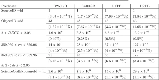
Table 4 shows the selectivity of queries while table 5 shows the selectivity of the predicates used by the queries.
4.6.1 SELECTION Queries
Table 6 shows the set of SELECTION queries used in our experiments. The query
Q1 retrieves information about a given Source (detection of sky objects) while queryQ2selects Sources (detection) and position (given by RA, DECL) of a given object. This query enables identifying moving objects. The query Q3 retrieves Objects and their detection (source) for a given sky area (bounded by RA and DECL). Q4 returns Detections (SourceID) and their positions from a given Sci-enceCDDExposure. The four queries target the Source Table.
Queries over non indexed data. From a SQL query,HiveandHadoopDBgenerate a MapReduce Job. Hive processes data SELECTION and PROJECTION within theMaptask, whereasHadoopDBincorporates, in theMaptask, database queries by using JDBC. A same query is sent to allMappers. TheReducefunction is not needed for the two systems because no additional processing is required after the Maptask.
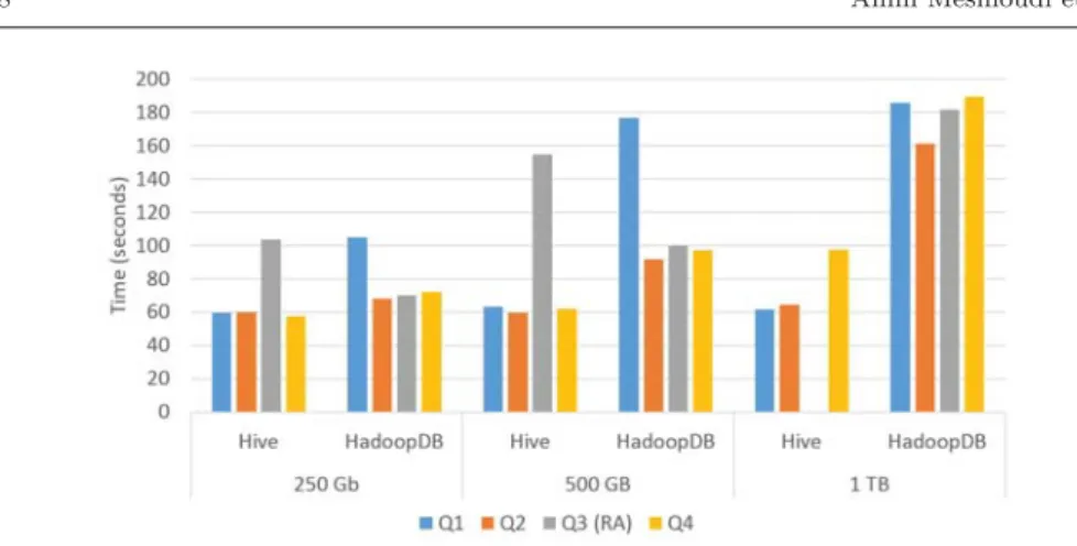
Figure 6 compares the execution time of the two systems (HadoopDBandHive) using three (3) datasets with 250 GB, 500 GB and 1 TB and a configuration of 50 nodes. We first executed the queries on no indexed data.
Regarding the dataset of 250 GB,HiveoutperformsHadoopDB. This is due to a latency of HadoopDB when it accesses to local DBMS using JDBC.Hive does not suffer from the same overhead since it directly accesses the data in theHDFS. However,HadoopDBoutperformsHivefor datasets of 500 GB and 1 TB. Indeed,
14 Additional results can be found in the project WebSite http://com.isima.fr/Petasky/
TASK Query D250GB D500GB D1TB D2TB SELECTION Q1 1 1 1 1 (3∗10−7%) (1.78∗10−7%) (7.69∗10−8%) (3.84∗10−8%) Q2 43 43 43 43 (1.2∗10−5%) (7.67∗10−6%) (3.3∗10−6%) (1.65∗10−6%) Q3 21 43 86 172 (6.6∗10−6%) (7.67∗10−6%) (6.61∗10−6%) (6.61∗10−6%) Q4 3.6 x 10³ 7.3 x 10³ 14.6 x 10³ 29.2 x 10³ (10−3%) (10−3%) (1.1∗10−3%) (1.1∗10−3%) GROUP BY Q5 2 2 4 6 (6.15∗10−7%) (3.57∗10−7%) (3.07∗10−7%) (2.3∗10−7%) Q6 9 x 10⁶ 18 x 106 36 x 106 58 x 106 (2.76%) (3.21%) (2.76%) (2.23%) JOIN Q7 43 43 86 215 (1.32∗10−5%) (7.7∗10−6%) (6.61∗10−6%) (8.26∗10−6%) Q8 28 x 103 28 x 103 57 x 103 127 x 103 (8∗10−3%) (5∗10−3%) (4∗10−3%) (4∗10−3%) Q9 7.7 x 10³ 7.7 x 10³ 7.7 x 10³ 7.7 x 10³ (2∗10−3%) (13∗10−3%) (6∗10−4%) (3∗10−4%) ORDER BY Q10 43 43 86 86 (1.32∗10−5%) (7.67∗10−6%) (6.61∗10−6%) (3.3∗10−6%) Q11 28 x 103 28 x 103 57 x 103 114 x 103 (8∗10−3%) (5∗10−3%) (4∗10−4%) (4∗10−3%)
Table 4:Selectivity of queries: For each query and for each data volume, the first line stands for the number of results and the second line stands for the percentage of results w.r.t the total number of records contained in the database
Predicate D250GB D500GB D1TB D2TB SourceID =id 1 1 1 1 (3.07∗10−7%) (1.7∗10−7%) (7.69∗10−8%) (3.84∗10−8%) ObjectID =id 43 43 43 43 (1.32∗10−2%) (7.67∗10−6%) (3.3∗10−6%) (1.65∗10−6%) 2< DECL <2.05 1.6 x 10⁶ 3.3 x 10⁶ 6.6 x 10⁶ 13.2 x 10⁶ (0.49%) (0.28%) (0.5%) (0.5%) 359.959< ra <359.96 14 x 103 28 x 103 57 x 103 127 x 103 (4∗10−3%) (2.5∗10−3%) (4∗10−3%) (4∗10−3%) 359.959< ra <359.96 21 43 86 172 (6.46∗10−6%) (3.5∗10−6%) (6.6∗10−6%) (3.3∗10−6%) & 2< decl <2.05 ScienceCcdExposureId = id 3.6 x 10³ 7.3 x 10³ 14.6 x 10³ 29.2 x 10³ (1.1∗10−3%) (6.4∗10−3%) (1.1∗10−3%) (1.1∗10−3%)
Table 5:Selectivity of predicates: For each predicates and for each data volume, the first line stands for the number of records satisfying the predicate and the second line stands for the those records w.r.t the total number of records contained in the database
Query SQL syntax
Q1 SELECT * FROM Source WHERE Sourceid=29785473054213321;
Q2 SELECT Sourceid, ra,decl FROM Source WHERE Objectid=402386896042823;
Q3 SELECT Sourceid, Objectid FROM Source WHERE ra >359.959 and ra<359.96 and decl<2.05 and decl>2;
Q4 SELECT Sourceid, ra,decl FROM Source WHERE scienceccdexposureid=454490250461;
Table 6: SELECTION queries
the use of the buffer and data compression (for 1 GB raw data, only 540 MB of disk space is used to store this data) makesHadoopDBmore efficient.
Regarding the scalability issue, we observe that if we double the data volume, the execution time increases in average by 250%. For example, the maximal time to query the dataset of 250 GB is 4 mins, whereas, the execution times observed for the same query over the datasets of 500 GB and 1 TB are respectively, 10 mins and 30 mins.
Queries over indexed data. Hive proceeds by filtering relevant parts of the index with respect to the condition expressed in a query. Only one index can be used to evaluate a query. The filtered part (keys, addresses) is then transferred to all the nodes of the cluster and only relevantHDFS blocks are processed. For example, query Q3 contains two filter conditions, one on the attribute RA and the other on the attribute DECL. We evaluated queryQ3 twice. In the first evaluation, we used the index on RA. Due to its size, which exceeds 1 GB (size of heap memory)
Fig. 7:SELECTION tasks with Index
for all the datasets, the workers choose to not use this index to evaluate queryQ3. In the second evaluation, we used an index on DECL. For the dataset of 1 TB, the size of the filtered part exceeds the size of the Heap memory.
InHadoopDB, indexes are automatically used by the local DBMS optimizer in each chunk.
Figure 7 shows the time needed to evaluate the queries using the indexes. One can observe that there is an improvement up to 70X forHive, whereas, the improvement is only of 9X forHadoopDB.
Regarding data scalability, we need only 1.3X of time if we have 2X of data. For example, the maximal time to query the dataset of 250 GB is 2 mins, whereas, the datasets of 500 GB and 1 TB need 3 mins and 3.5 mins respectively.
Hive outperforms HadoopDBexcept for the query Q3. In most cases, in par-ticular for selective queries, a global index (proposed inHive) leads to better per-formances than a local index (proposed inHadoopDB). However, the limit of this strategy is that when the size of the filtered part becomes larger, the nodes are no longer able to manage the indexes.
4.6.2 Aggregate Queries
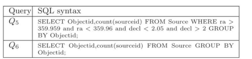
Table 7 shows the two considered aggregate queries. QueryQ5computes the num-ber of observations (sources) of a given bounded area of the sky. Only a few tuples (<10) are expected as a result for this query. The considered area is extended in the query Q6, where the expected number of tuples to be returned by the query ranges from 9 to 58 millions of tuples.
Both Hive and HadoopDB use only one MapReduce Job to implement each of these queries. In the Map step, Hive performs data read, PROJECTION and filtering and as well as a partial GROUP BY. In theReducestep, a global GROUP BY is performed. The number ofMap tasks depends on the number of blocks of data in theHDFS. For example, for the 250 GB dataset, 887Maptasks have been executed, whereas the number of Reduce tasks is determined by Hive using two parameters: the size ofMapInput data and the maximum size of data handled by aReducer(Hive.exec.reducers.bytes.per.reducer). For the dataset with 250 GB, we
Query SQL syntax
Q5 SELECT Objectid,count(sourceid) FROM Source WHERE ra> 359.959 and ra<359.96 and decl<2.05 and decl>2 GROUP BY Objectid;
Q6 SELECT Objectid,count(sourceid) FROM Source GROUP BY Objectid;
Table 7:Aggregation queries
have 236 Reducetasks obtained from the size of the Source table (i.e., 236 GB) and the size of data handled by aReducer(i.e., 1 GB).
ForHadoopDB, within theMapstep, the same query is sent to the local DBMS where PROJECTION, SELECTION and partial GROUP BY are performed. In theReduce step, the global GROUP BY is performed. The number ofMaptasks depends on the number of chunks (and subchunks) created in the data loading phase. For example, for the 250 GB dataset we have 250Maptasks, whereas the number ofReducetasks is set to one (1) byHadoopDB. ForHive, and because of its size, the index ObjectID cannot be used for the queryQ6. For example, for the 250 GB dataset, the size of the ObjectID index is equal to 5 GB. ForQ5, only RA can be used and only for the datasets with the sizes 250 GB and 500 GB. Indeed, the sizes of the filtered part of indexes of DECL and ObjectID exceed the heap memory dedicated to theMapper(>1 GB).
A comparison of the execution time of queriesQ5andQ6 is shown on figure 8. We can observe that, for selective queries (e.g., queryQ5),HadoopDBoutperforms Hivefor both indexed and non indexed data. Indeed, due to the few tuples (<10) transferred fromMappers to Reducers, the time needed to handle theMap tasks represents the most important part of the total time needed to process the whole query. The ability ofHadoopDB, unlikeHive, to process compressed data (e.g., for the dataset with 1 TB, 554 GB of compressed data forHadoopDBand 944 GB of non-compressed data forHive) in theMapphase makesHadoopDBmore efficient. The difference in performances of HadoopDB compared to Hive can reach up to 15X, with a maximum of 35 mins of processing time forHive and 12.5 mins for HadoopDB.
Due to the size of data transferred fromMapperstoReducers(e.g., 9 GB trans-ferred in the case of the dataset of 1 TB), the time needed to handle theReduce tasks impacts the global time needed to perform the whole query. Indeed, for non-selective queries (e.g., queryQ6),Hiveparallelizes the processing of GROUP BY in theReducephase by using all the nodes of the cluster asReducers, whereas, for HadoopDBonly one node is used as aReducer. In the case of non-indexed data, Hive is significantly better than HadoopDB (with and without indexes). Indexes are useless in this case because all the records must be accessed (full scan). The difference in performances of Hive compared to HadoopDB can reach up to 2X, with a maximum of 36 mins forHiveand 1 hour 10 mins forHadoopDB.
Regarding data scalability, we need in average only 2X of time if we have 2X of data. For example, the maximum time to query the dataset of 250 GB is 20 mins, whereas, the datasets with 500 GB and 1 TB need 40 mins and 1 hour 10 mins respectively.
In the case of non selective queries, the use of only one Reducer represents a bottleneck for HadoopDB. To optimize this kind of queries, HadoopDBproposes
Fig. 8:GROUP BY tasks: Hive vs. HadoopDB
Fig. 9:GROUP BY optimization within HadoopDB vs. Hive
to modify the partitioning attribute. Indeed, our results were obtained while the Source table is partitioned using the SourceID attribute. When we change the partitioning attribute to ObjectID, we observe an improvement over the previous results, which can reach up to 5X. The results are shown in figure 9. The modi-fication of the partitioning attribute allows:(i)to minimize the number of <key, value> transferred from Mappers to the Reducer and therefore the size of data to be processed by the Reducer, and (ii) to avoid the global GROUP BY in the Reducerside which was already done by theMappers.
4.6.3 JOIN Queries
Table 8 shows the considered JOIN queries. QueriesQ7 and Q5 express a JOIN between the tablesSourceandObject. The two queries retrieve information about objects and their observations (sources). In queryQ7, the sky area is constrained
Query SQL syntax
Q7 SELECT * FROM Source JOIN Object on (source.objectid=object.objectid) WHERE ra > 359.959 and ra<359.96 and decl<2.05 and decl>2;
Q8 SELECT * FROM Source JOIN Object on (source.objectid=object.objectid) WHERE ra > 359.959 and ra<359.96;
Q9 SELECT s.psfFlux, s.psfFluxSigma, sce.exposureType FROM Source s JOIN RefSrcMatch rsm ON (s.sourceId = rsm.sourceId) JOIN Science Ccd Exposure Metadata sce ON (s.scienceCcdExposureId = sce.scienceCcdExposureId) WHERE s.ra>359.959 and s.ra <359.96 and s.decl< 2.05 and s.decl>2 and s.filterId = 2 and rsm.refObjectId is not NULL;
Table 8: JOIN queries
Fig. 10:JOIN tasks
by RA and DECL, whereas in queryQ8, the sky area is constrained only by RA. The sky area of query Q7 is included in the sky area of query Q8. Query Q9 expresses a JOIN between three tables: Source, Science Ccd Exposure Metadata and RefSrcMatch. This query retrieves the Sources, from a given sky area, and their related metadata obtained from Science Ccd Exposure Metadata and RefS-rcMatch.
HadoopDBdoes not support queries with Joins involving more than two tables, therefore the queryQ9 is not considered.
The number ofMapReduce Jobs generated byHivedepends on the number of Joins in the query. For each JOIN, Hivecreates a Job. Therefore, for queries Q7 and Q8,Hivegenerates only one (1) job while it generates two (2) jobs for query
Q9. In the case of two Joins or more, the result of each JOIN is used as an input for the next JOIN.Hivestores the partial results in theHDFS.
In theMapstep,Hiveperforms data read, PROJECTION, filtering and tuples hashing (to group together tuples with same values of the JOIN key), while in the
Query SQL syntax
10 SELECT Objectid,sourceid FROM Source WHERE ra> 359.959 and ra<359.96 and decl< 2.05 and decl>2 ORDER BY Objectid;
11 SELECT Objectid,sourceid FROM Source WHERE ra> 359.959 and ra<359.96 ORDER BY Objectid;
Table 9:ORDER BY queries
Reducestep, a join is performed. The number ofMaptasks depends on the number of blocks of data in the HDFS(e.g., for the 250 GB dataset and queries Q7 and
Q8, we have 938 Map tasks) whereas the number ofReduce tasks is set byHive (e.g., for the 250 GB dataset and queriesQ7 andQ8, we have 252Reducetasks)
For HadoopDB, within the Map phase, the same Query is sent to the local DBMS where PROJECTION and SELECTION are performed. In the Reduce step, the JOIN is performed. The number ofMaptasks depends on the number of chunks (and subchunks) created in the data loading phase (e.g., for the 250 GB dataset we have 250Maptasks) whereas the number ofReducetasks is set to one (1) byHadoopDB.
Figure 10 shows the execution time of the considered join queries. Hive out-performs HadoopDB for both queries Q7 and Q8. Indeed, for the query Q7 the difference of performance can reach 1.7X, whereas for the queryQ8, the difference can exceed 12X.
As noticed for the GROUP BY queries, when the size of the result returned by theMappersis large, the one-Reducestrategy adopted byHadoopDBbecomes problematic and represents a bottleneck.
4.6.4 ORDER BY Queries
Table 9 shows our queries for the ORDER BY task. These queries retrieve objects and their detections (sources) ordered by ObjectID. Query Q10, considers a sky area bounded by RA and DECL, whereas query Q11 considers a larger sky area bounded only by RA. BothHadoopDBandHivegenerate only oneMapReduceJob from these queries. In the Map step, Hive performs data READ, SELECTION, PROJECTION operations and a partial ORDER BY, whereasHadoopDBsends the same query to all local DBMSs. The number of Map tasks depends on the number of data blocs in the HDFS (e.g., for the dataset with 250 GB, we have 887Maptasks). WithHadoopDB, the number of tasks depends on the number of chunks created in the data loading stage. In theReducestep, a global ORDER BY is performed by both systems using only oneReducer.
Due to their sizes,Hivecan use indexes only for the datasets with 250 GB and 500 GB. For the 1 TB dataset, the size of the filtered part exceeds the size of heap memory used by theMapper.
Figure 11 shows the evolution of execution time forHadoopDBand Hiveover non indexed and indexed datasets. We observe that HadoopDB is significantly better thanHivewith and without indexes.
With the index, a gain of 7X is reported forHiveand a gain of 11X is reported for HadoopDB. Furthermore, HadoopDBoutperformsHivewith a factor that can exceed 2X.
Fig. 11:ORDER BY tasks
5 Discussion
In this section, we first summarize the query evaluation mechanisms for SQL On MapReduce systems and the impact of different proposed optimization techniques on query evaluation. Then, we analyze the limits of these techniques with respect to LSST needs. We also make some proposals that could contribute to the design of a system able of meeting the LSST requirements in terms of data management. In the LSST project, data is collected and exploited progressively. Indeed, an amount of 15 TB is expected to be collected each night. This data must be inte-grated with the already available one. In the sequel, we call such a data integration process: anintegration iteration. Roughly speaking, to perform anintegration it-eration there is a need to process (index, compress, partition) the new data and integrate it with already available data.
We first start by analyzing the loading time. With respect to LSST data, both approaches proposed byHiveand HadoopDBare compatible with new data integration. HoweverHadoopDB, is not efficient with respect to all kinds of queries, because when data is partitioned using a given attribute (e.g., objectID), in the next integration iteration, there is no guarantee that all the records with the same partitioning key are in the same local database. A partitioning is efficient with respect to new data but not for all the data stored in the database (old and new data). Therefore, it is questionable whether it is really worth to have a customized data partitioning strategy when data is collected and integrated progressively. The only method that enables to guarantee the optimality of query processing, is a redistribution (i.e., repartitioning) of all the available data each night. This solution is clearly not feasible due to induced time overhead: data loading time increases exponentially with respect to data volume. Indeed, more than 200-300% of the time is spent in partitioning data for a final result which is not necessarily very relevant.
Regarding indexing strategies, and with respect to data integration iteration, the strategy of HadoopDBremains very consistent. If we assume that partition-ing does not trigger any particular problem, the data indexpartition-ing strategy becomes even more interesting. Indeed, indexes are created at chunk level. When an index
is created, the existing indexes are not impacted and hence there is no need to recalculate them. In contrast, the strategy of creating indexes inHiveis not com-patible with integration constraints. Indeed, to ensure that an index will be used, it is necessary to recalculate it. Moreover,Hiveis not stable in using indexes. The indexing mechanism ofHiveshould be revisited with respect to these constraints and extended with additional functionalities such as: multiple index (with multi-ple attributes), automatic selection of indexes, integration of indexes in additional operators (currently only the selection operator supports the use of indexes).
The index size is exponential with respect to the number of distinct values. We have to study new compressed structures. Indeed, 10% of space overhead for storing one index is not a realistic solution in particular in the case of tables with hundreds of attributes and which require several indexes. The size of indexes in HadoopDBis however very acceptable (3.2% of the overall size of a raw chunk). Moreover,HadoopDBsupports multiple indexes, but the usage of indexes is how-ever still limited to selection queries. The benefit of indexing inHiveis to provide a global view about data location with however a price to pay in terms of sizes of indexes and maintenance since there is a need to recalculate an index at each inte-gration iteration step. Indexes proposed inHadoopDBdo not require a large size and are calculated quickly which is compatible with integration iteration steps. Nevertheless,HadoopDBindexes do not provide a global view of the data.
We believe that a hierarchical indexing, with several levels, may offer a good compromise. Such an index structure can take advantages from the global view of data offered byHiveand the ease of use offered byHadoopDB.
Before comparing the execution time of the considered systems, we will first introduce some cost metrics which will be used to analyze the various query eval-uation and optimization strategies ofHiveand HadoopDB.
First of all, as mentioned previously, an SQL query is mapped to a set of MapReduce jobs. In each MapReduce job, we have five steps: (i) Data is read and transferred toMappersas key/value pairs. We denote by CostRead Data, the cost of this step.(ii) A Map function is applied on the data read and key/value pairs received by the Mapper. We denote this cost by Cost Map. (iii)A network synchronization by sending key/value pairs generated by the mappers toReducers. We denote by Cost network, the cost of this step. (iv) The reduce function is applied. We denote this cost by Cost reduce.(v)Partial results are written in the HDFS, these results will be, if necessary, used as input for the next job. We denote this cost by Cost WriteHDFS. These five steps are not required for all the queries. Indeed, for JOIN queries, we need all the steps, while for SELECTION queries only steps (i) and (ii) are required.
The overall cost of a job is obtained by summing these five costs. We denote this cost by Cost Job. Finally, we define the cost related to query processing as the sum of all costs of all jobs associated with the query. In the rest of this paper, we discuss the impact of each cost with respect to query types.
In the case of selection queries, and without considering indexes, only one job is generated both in the case of Hive and HadoopDB. In this case, the cost of a query is the same as the cost of its associated job. In the implementation of such a job, the two systems read data and applies the filtering associated with predicates in the query. Consequently the cost of such a job is: CostRead Data + Cost Map. The CostRead Data, inHadoopDB, is given by the time necessary to read data from DBMS using JDBC. For Hive, this cost is related to chunks reading from
the HDFS. As data in the DBMS is compressed, the CostRead Data related to HadoopDB job is less than CostRead Data related to Hive in most cases. The only different case is when CostRead Data, forHadoopDB, is dominated by JDBC latencies.
Both tools propose to use indexes to minimize CostRead Data. Indeed, in HadoopDB, indexes are used within the DBMS which allow to only access rel-evant disk pages by the DBMS. ForHive, we use an additional data structure that allows to locate only relevant HDFS chunks. In this vein, a filtering phase is used before applying the Map function. The Cost CostRead Data is minimized using the index. We have seen that whenHivedecides to use an index, the result is better becauseHive has a global view of the data which enables to locate relevant data more efficiently compared toHadoopDB.
The drawback of Hiveis when the filter part has an important size. Indeed, when reading data,Hiveextracts relevant chunks and sub-chunks, from index, that satisfy predicates in the query. If the filtered part cannot fit into the memory of Mappers,Hiveis not able to use indexes. To conclude, we need a more sophisticated optimizer that can decide when a usage of an index is relevant and which index to use. In addition, Hive indexing mechanism must be extended to enable complex indexes with multiple attributes.
Another important point, for LSST project, is the choice of attributes to index. As some queries are known, it will be very interesting to have an index recommen-dation system for a large number of attributes.
With respect to GROUP BY queries, both Hive and HaddopDB read data, apply the filter related to predicates in a query and then apply partial GROUP BY, in theMapside. They send then the data to theReducer(s)where a global GROUP BY is applied. Only one job is used, therefore the cost of a query is equivalent to the cost of the associated job. The cost of such a job is then: CostRead Data + Cost Map + Cost network + Cost reduce. For selective queries, only a few (<10) tuples are transferred fromMappers to Reducers. Therefore, CostRead Data and Cost Map dominate the Job cost. By compressing data HadoopDB outperforms Hive.
With respect to non-selective queries, the data transferred from Mappers to Reducersimpacts the performance of the generated jobs. As HadoopDBuses one Reducer to perform the global GROUP BY and Hive uses several Reducers, we have observed that even when an index is used in HadoopDB, Hive outperforms HadoopDBfor non-selective queries. Indeed, Cost reduce is shared between several machines, whereas for HadoopDB, due to the use of a single Reducer, this cost dominates the query processing cost and constitutes a bottleneck.
HadoopDBproposes to modify the partitioning attribute to deal with GROUP BY queries. Indeed, by changing the partitioning attribute, we are sure that most records having the same GROUP BY key are in the same node and hence there is no need to perform a global GROUP BY for the concerned records. In this case, the number of key/values transferred fromMapperstoReducersis minimized. We have observed a very significant gain in this case. The cost of network transfer and reduce phases are minimized using this technique. The drawback of this strategy comes from the fact that it requires to identifya priorithe adequate partitioning attribute.
Determining a good partitioning strategy for LSST data is very challenging knowing that in LSST, several attributes are used as grouping attributes. It will
be interesting to study the problem of partitioning data starting from a set of predefined queries. Another issue is related to the identification of the adequate number ofReducersto use for each query. In current state of affairs,Hiveleaves this choice to the user. Extending such a system in order to be able to automatically determine the optimal number ofReducersto use during query execution is indeed an interesting research issue.
Regarding JOIN queries,Hivegenerates, for each JOIN, aMapReducejob. HadoopDB does not support joins of more than two tables and do not allow multiple Reducersto perform the reduce function. Indeed, for JOIN queries and to the best of our knowledge, there is no optimization technique implemented in the open source release ofHadoopDB. Also indexes are not used to perform joins. The cost of JOIN queries is obtained by the sum of costs of the associated jobs. Intermediate results are stored in the HDFS. In this case, the order of joining the relations has an important impact on query performances. To the best of our knowledge, no relevant techniques for finding the best order of joining tables is proposed so far. We believe that the optimizer of Hive should be revisited to incorporate sophisticated scheduling technique based on statistics. Indeed, the order of evaluation of joins will significantly impact query performance. In the TEZ system, Beta-version ofHadoop,MapReducetasks can be pipelined without going through the store in the HDFS.
Regarding ORDER BY queries, both approaches propose to handle these queries in one job.HadoopDBoutperformsHive becauseHadoopDBtakes advan-tages of compression and indexing, handled by the DBMS and minimizes the cost of CostRead Data. The ORDER BY in theMap phase is not mandatory because it can be performed by the DBMS when it reads the data. We believe that the MapReducemodel is not suitable for handling JOIN and ORDER BY queries. We believe that this model is efficient for queries that need only one pass on the data (e.g., Selection and GROUP BY).
Another issue is the optimization of UDF (User Defined Functions). Indeed, UDF are very frequently used in astrophysics applications. Optimization within theMapReduceframework is not an easy task. WithinHive, we implemented some UDFs and we successfully executed those queries in a declarative manner. Hive offers several kinds of UDF: UDFs that can be evaluated in theMapphase, in the Reducephase and as a separated job. For HadoopDB, the integration of UDFs is achieved manually as a separateMapReduceJob.HadoopDBlacks mechanisms for evaluating queries declaratively.
With respect to query frequency, in LSST we expect a half million of queries per day. At any time, we expect that the system should handle 50 simple queries (that need a few seconds to be evaluated) and 20 complex query (that could require hours or days to be evaluated). The versions ofHadoopused in our experiments are not able to support execution of multi-jobs. Actually, another version ofHadoop, called Yarn, provides this ability. Therefore, it will be interesting to investigate global execution and optimization of sets of queries in aMapReduceframework.
6 Conclusion
We designed and set up a benchmark for structured data from astronomy where a set of SQL queries are already defined. Our experiments targeted two