Regularization in Matrix Relevance Learning
Petra Schneider, Kerstin Bunte, Han Stiekema, Barbara Hammer, Thomas Villmann and Michael Biehl
Abstract—We present a regularization technique to extend
recently proposed matrix learning schemes in learning vector quantization (LVQ). These learning algorithms extend the con-cept of adaptive distance measures in LVQ to the use of relevance matrices. In general, metric learning can display a tendency towards over-simplification in the course of training. An overly pronounced elimination of dimensions in feature space can have negative effects on the performance and may lead to instabilities in the training. We focus on matrix learning in Generalized LVQ. Extending the cost function by an appropriate regularization term prevents the unfavorable behavior and can help to improve the generalization ability. The approach is first tested and illustrated in terms of artificial model data. Furthermore, we apply the scheme to benchmark classification data sets from the UCI Repository of machine learning. We demonstrate the usefulness of regularization also in the case of rank limited relevance matrices, i.e. matrix learning with an implicit, low dimensional representation of the data.
Index Terms—Learning Vector Quantization, metric
adapta-tion, cost funcadapta-tion, regularization
I. INTRODUCTION
Learning Vector Quantization (LVQ) as introduced by Ko-honen is a particularly intuitive and simple though powerful classification scheme [1]. A set of so-called prototype vectors approximate the classes of a given data set. The prototypes parameterize a distance-based classification scheme, i.e. data is assigned to the class represented by the closest prototype. Unlike many alternative classification schemes, such as feed-forward networks or the Support Vector Machine (SVM) [2], LVQ systems are straightforward to interpret. Since the basic algorithm was introduce in 1986 [1], a huge number of modifications and extensions has been proposed, see e.g. [3], [4], [5], [6]. The methods have been used in a variety of academic and commercial applications such as image analysis, bioinformatics, medicine, etc. [7], [8].
Metric learning is a valuable technique to improve the basic LVQ approach of nearest prototype classification: a parameterized distance measure is adapted to the data to optimize the metric for the specific application. Relevance learning allows to weight the input features according to their importance for the classification task [5], [9]. Especially in case of high dimensional, heterogeneous real life data this approach turned out particularly suitable, since it accounts for irrelevant or inadequately scaled dimensions; see [10], [11] for applications. Matrix learning additionally accounts for
P. Schneider, K. Bunte, H. Stiekema and M. Biehl are with the Johann Bernoulli Institute for Mathematics and Computer Science, University of Groningen, P.O. Box 407, 9700 AK Groningen, The Netherlands
B. Hammer is with the University of Bielefeld, Faculty of Technology, CITEC, 33594 Bielefeld, Germany
T. Villmann is with the Department of Mathematics/Physics/Computer Science, University of Applied Sciences Mittweida, Technikum Platz 17, 09648 Mittweida, Germany
pairwise correlations of features [6], [12]; hence, very flexible distance measures can be derived.
However, metric adaptation techniques may be subject to over-simplification of the classifier as the algorithms possibly eliminate too many dimensions. A theoretical investigation for this behavior can be found in [13].
In this work, we present a regularization scheme for metric adaptation methods in LVQ to prevent the algorithms from over-simplifying the distance measure. We demonstrate the behavior of the method by means of an artificial data set and real world applications. It is also applied in the context of rank limited relevance matrices, which realize an implicit low-dimensional representation of the data.
II. MATRIX LEARNING INLVQ
LVQ aims at parameterizing a distance-based classifica-tion scheme in terms of prototypes. Assume training data
{ξi, yi}li=1∈Rn× {1, . . . , C}are given,ndenoting the data
dimension andC the number of different classes. An LVQ
network consists of a number of prototypes which are char-acterized by their location in the feature space wi ∈Rn and
their class labelc(wi)∈ {1, . . . , C}. Classification takes place
by a winner takes all scheme. For this purpose, a (possibly parameterized) distance measure d is defined in Rn. Often, the squared Euclidean metric d(w, ξ) = (ξ−w)T(ξ−w)
is chosen. A data pointξ∈Rn is mapped to the class label c(ξ) =c(wi)of the prototypeifor whichd(wi, ξ)≤d(wj, ξ)
holds for everyj6=i(breaking ties arbitrarily). Learning aims at determining weight locations for the prototypes such that the given training data are mapped to their corresponding class labels.
Training of the prototype positions in feature space is often guided by heuristic update rules, e.g. in LVQ1 and LVQ2.1 [1]. Alternatively, researchers have proposed variants of LVQ which can be derived from an underlying cost function. Generalized LVQ (GLVQ) [3] e.g., is based on a heuristic cost function which can be related to a maximization of the hypothesis margin of the classifier. Mathematically well-founded alternatives were proposed in [4] and [14]: the cost functions of Soft LVQ and Robust Soft LVQ are based on a statistical modelling of the data distribution by a mixture of Gaussians, and training aims at optimizing the likelihood.
However, all these methods rely on a fixed distance, e.g. the standard Euclidean distance which may be inappropriate if the data does not display a Euclidean characteristic. The squared weighted Euclidean metricdλ(
w, ξ) =Piλi(ξi−wi)2 with
λi≥0andPiλi = 1allows to use prototype based learning also in the presence of high dimensional data with features of different, yet a priori unknown, relevance. Extensions of LVQ1 and GLVQ with respect to this metric were proposed
in [5], [9], called Relevance LVQ (RLVQ) and Generalized Relevance LVQ (GRLVQ).
Matrix learning in LVQ schemes was introduced in [6], [12]. Here, the Euclidean distance is generalized by a full matrixΛ
of adaptive relevances. The new metric reads
dΛ(w, ξ) = (ξ−w)TΛ (ξ−w), (1)
whereΛis ann×nmatrix. The above dissimilarity measure
only corresponds to a meaningful distance, if Λ is positive
semi-definite. This can be achieved by substitutingΛ = ΩTΩ,
whereΩ∈Rm×n withm≤nis an arbitrary matrix. Hence,
the distance measure reads dΛ( w, ξ) = n X i,j m X k (ξi−wi)ΩkiΩkj(ξj−wj). (2)
Note, that Ω realizes a coordinate transformation to a new
feature space of dimensionality m ≤ n. The metric dΛ
corresponds to the squared Euclidean distance in this new coordinate system. This can be seen by rewriting Eq. (1) as follows:
dΛ(
w, ξ) =(ξ−w)TΩT Ω(ξ−w).
Using this distance measure, the LVQ classifier is not restricted to the original set of features any more to classify the data. The system is able to detect alternative directions in feature space which provide more discriminative power to separate the classes. Choosingm < nimplies that the classifier is restricted to a reduced number of features compared to the original input dimensionality of the data. Consequently, rank(Λ)≤m
and at least (n−m) eigenvalues of Λ are equal to zero.
In many applications, the intrinsic dimensionality of the data is smaller than the original number of features. Hence, this approach does not necessarily constrict the performance of the classifier extensively. In addition, it can be used to derive low-dimensional representations of high-low-dimensional data [15].
Moreover, it is possible to work with local matrices attached to the individual prototypes. In this case, the squared distance of data pointξfrom the prototypewjreadsdΛj(wj, ξ) = (ξ− wj)Λj(ξ−wj). Localized matrices have the potential to take
into account correlations which can vary between different classes or regions in feature space.
LVQ schemes which optimize a cost function can easily be extended with respect to the new distance measure. To obtain the update rules for the training algorithms, the derivatives of
(1) with respect to wandΩhave to be computed. We obtain
∂dΛ(w, ξ) ∂w =−2 Λ (ξ− w) =−2 ΩTΩ (ξ−w), (3) ∂dΛ( w, ξ) ∂Ωlm = 2X i (ξi−wi)Ωli(ξm−wm). (4) Note however that Eq. (4) only holds for an unstructured matrix Ω. In the special case of quadratic, symmetricΩ, the off-diagonal elements cannot be varied independently. In con-sequence, diagonal and off-diagonal elements yield different derivatives. However, this special case is not considered in this study. In the following, we always refer to the most general case of arbitrary Ω∈Rm×n.
Additionally, in the course of training,Λhas to be normal-ized after every update step to prevent the learning algorithm
from degeneration. Possible approaches are to set P
iΛii or
det(Λ)to a fixed value, hence, either the sum of eigenvalues or the product of eigenvalues is constant.
In this paper, we focus on matrix learning in Generalized LVQ. In the following, we shortly derive the learning rules.
A. Matrix learning in Generalized LVQ
Matrix learning in GLVQ is derived as a minimization of the cost function E= l X i=1 φ dΛ J(ξi)−dΛK(ξi) dΛ J(ξi) +dΛK(ξi) , (5)
whereφis a monotonic function, e.g. the logistic function or the identity, dΛ
J(ξ) = d
Λ(w
J, ξ)is the distance of data point
ξ from the closest prototype wJ with the same class label
y, and dΛ
K(ξ) = d
Λ(w
K, ξ) is the distance from the closest prototype wK with any class label different from y. Taking
the derivatives with respect to the prototypes and the metric parameters yields a gradient based adaptation scheme. Using Eq. (3), we get the following update rule for the prototypes
wJ andwK ∆wJ = +α1·φ′(µ(ξ))·µ+(ξ)·Λ·(ξ−wJ), (6) ∆wK = −α1·φ′(µ(ξ))·µ−(ξ)·Λ·(ξ−wK), (7) withµ(ξ) = (dΛ J −dΛK)/(dΛJ +dΛK), µ+(ξ) = 4·dΛK/(dΛJ + dΛ K)2, and µ − (ξ) = 4·dΛ J/(dΛJ +dΛK)2; α1 is the learning rate for the prototypes. Throughout the following, we use the identity function φ(x) = x which implies φ′
(x) = 1. The update rule for non-structuredΩresults in
∆Ωlm=− α2·φ′(µ(ξ))· (8) µ+(ξ)·(ξ m−wJ,m)[Ω(ξ−wJ)]l −µ− (ξ)·(ξm−wK,m)[Ω(ξ−wK)]l ! , whereα2 is the learning rate for the metric parameters. Each update is followed by a normalization step to prevent the algorithm from degeneration. We call the extension of GLVQ defined by Eq.s (6), (7) and (8) Generalized Matrix LVQ (GMLVQ) [6].
In our experiments, we also apply local matrix learning in GLVQ with individual matricesΛjattached to each prototype; again, the training is based on non-structuredΩj. In this case, the learning rules for the metric parameters yield
∆ΩJ,lm=−α2·φ ′ (µ(ξ))· µ+(ξ)·(ξm−wJ,m)[ΩJ(ξ−wJ)]l , (9) ∆ΩK,lm= +α2·φ′(µ(ξ))· µ− (ξ)·(ξm−wK,m)[ΩK(ξ−wK)]l . (10) Using this approach, the update rules for the prototypes also include the local matrices. We refer to this method as localized GMLVQ (LGMLVQ) [6].
III. MOTIVATION
The standard motivation for regularization is to prevent a learn-ing system from over-fittlearn-ing, i.e. the overly specific adaptation to the given training set. In previous applications of matrix learning in LVQ we observed only weak over-fitting effects. Nevertheless, restricting the adaptation of relevance matrices can help to improve generalization ability in some cases.
A more important reasoning behind the suggested regular-ization is the following: in previous experiments with different metric adaptation schemes in Learning Vector Quantization it has been observed, that the algorithms show a tendency to over-simplify the classifier [16], [6], i.e. the computation of the distance values is finally based on a strongly reduced number of features compared to the original input dimensionality of the data. In case of matrix learning in LVQ1, this conver-gence behavior can be derived analytically under simplifying assumptions [13]. The elaboration of these considerations is ongoing work and will be topic of further forthcoming publica-tions. Certainly, the observations described above indicate that the arguments are still valid under more general conditions. Frequently, there is only one linear combination of features remaining at the end of training. Depending on the adaptation of a relevance vector or a relevance matrix, this results in a single non-zero relevance factor or eigenvalue, respectively. Observing the evolution of the relevances or eigenvalues in such a situation shows that the classification error either remains constant while the metric still adapts to the data, or the over-simplification causes a degrading classification perfor-mance on training and test set. Note that these observations do not reflect over-fitting, since training and test error increase concurrently. In case of the cost-function based algorithms this effect could be explained by the fact that a minimum of the cost function does not necessarily coincide with an optimum in matters of classification performance. Note that the numerator in Eq. (5) is smaller than 0 iff the classification of the data point is correct. The smaller the numerator, the greater the security of classification, i.e. the difference of the distances to the closest correct and wrong prototype. While this effect is desirable to achieve a large separation margin, it has unwanted effects when combined with metric adaptation: it causes the risk of a complete deletion of dimensions if they contribute only minor parts to the classification. This way, the classification accuracy might be severely reduced in exchange for sparse, ’over-simplified’ models. But over-simplification is also observed in training with heuristic algorithms [16]. Training of relevance vectors seems to be more sensitive to this effect than matrix adaptation. The determination of a new direction in feature space allows more freedom than the restriction to one of the original input features. Nevertheless, degrading classification performance can also be expected for matrix adaptation. Thus, it may be reasonable to improve the learning behavior of matrix adaptation algorithms by preventing strong decays in the eigenvalue profile of Λ.
In addition, extreme eigenvalue settings can invoke numer-ical instabilities in case of GMLVQ. An example scenario, which involves an artificial data set, will be presented in the Sec. V-A. Our regularization scheme prevents the matrix
Λ from becoming singular. As we will demonstrate, it thus
overcomes the above mentioned instability problem.
IV. REGULARIZEDCOSTFUNCTION
In order to derive relevance matrices with more uniform eigen-value profiles, we make use of the fact that maximizing the determinant of an arbitrary, quadratic matrixA∈Rn×n with eigenvalues ν1, . . . , νn suppresses large differences between the νi. Note that det(A) = Qiνi which is maximized by
νi= 1/n,∀iunder the constraintPiνi = 1. Hence, maximiz-ingdet(Λ)seems to be an appropriate strategy to manipulate the eigenvalues ofΛthe desired way, whenΛis non-singular.
However, since det(Λ) = 0 holds for Ω ∈ Rm×n with
m < n, this approach cannot be applied, if the computation of Λ is based on a rectangular matrix Ω. However, the first
m eigenvalues of Λ = ΩTΩ are equal to the eigenvalues
of ΩΩT ∈ Rm×m. Hence, maximizing det(ΩΩT) imposes
a tendency of the firstm eigenvalues ofΛ to reach the value
1/m. Since det(Λ) = det(ΩTΩ) = det(ΩΩT) holds for
m = n, we propose the following regularization term θ in
order to obtain a relevance matrixΛwith balanced eigenvalues close to 1/nor1/mrespectively:
θ= ln det ΩΩT
. (11)
The approach can easily be applied to any LVQ algorithm
with an underlying cost function E. Note that θ has to be
added or subtracted depending on the character of E. The
derivative with respect toΩyields ∂θ ∂Ω = ∂ln(det(ΩΩT)) ∂det(ΩΩT) ∂det(ΩΩT) ∂ΩΩT ∂ΩΩT ∂Ω = 2·(Ω+)T,
where Ω+ denotes the Moore-Penrose pseudo-inverse of Ω.
For the proof of this derivative we refer to [17]. Sinceθ only depends on the metric parameters, the update rules for the prototypes are not affected.
In case of GMLVQ, the extended cost function reads
˜
E =E−η
2 ·ln det ΩΩ
T
. (12)
The regularization parameter η adjusts the importance of the different goals covered by E˜. Consequently, the update rule for the metric parameters given in Eq. (8) is extended by
∆Ωθ,lm= +α2·η·Ω+ml. (13) The regularization parameter has to be optimized by means of a validation procedure.
The concept can easily be transfered to relevance LVQ with exclusively diagonal relevance factors [5], [9]: in this case, the
regularization term readsθ = ln(Q
iλi), because the weight factors λi in the scaled Euclidean metric correspond to the eigenvalues ofΛ. In the experimental section, we also examine regularization in GRLVQ.
Sinceθis only defined in terms of the metric parameters, it can be expected that the number of prototypes does not have significant influence on the application of the regularization technique. This claim will be verified by means of a real life classification problem in Sec. V-B3.
−5 0 5 −10 −5 0 5 Class 1 Class 2 (a) −5 0 5 −10 −5 0 5 Class 1 Class 2 (b) −5 0 5 −10 −5 0 5 Class 1 Class 2 (c) −5 0 5 −10 −5 0 5 Class 1 Class 2 (d) −5 0 5 −10 −5 0 5 Class 1 Class 2 (e) −5 0 5 −10 −5 0 5 Class 1 Class 2 (f) −5 0 5 −10 −5 0 5 Class 1 Class 2 (g) −5 0 5 −10 −5 0 5 Class 1 Class 2 (h) −5 0 5 −10 −5 0 5 Class 1 Class 2 (i) −5 0 5 −10 −5 0 5 Class 1 Class 2 (j)
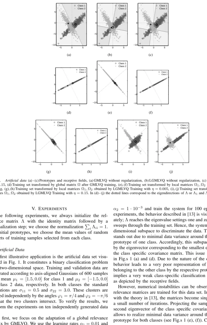
Fig. 1. Artificial data (a) - (c) Prototypes and receptive fields, (a) GMLVQ without regularization, (b) LGMLVQ without regularization, (c) LGMLVQ with η= 0.15, (d) Training set transformed by global matrixΩafter GMLVQ training, (e), (f) Training set transformed by local matricesΩ1,Ω2 after LGMLVQ
training, (g), (h) Training set transformed by local matricesΩ1,Ω2 obtained by LGMLVQ Training withη= 0.005, (i), (j) Training set transformed by local
matricesΩ1,Ω2obtained by LGMLVQ Training withη= 0.15. In (d) - (j) the dotted lines correspond to the eigendirections ofΛorΛ1andΛ2, respectively.
V. EXPERIMENTS
In the following experiments, we always initialize the
rel-evance matrix Λ with the identity matrix followed by a
normalization step; we choose the normalizationP
iΛii= 1. As initial prototypes, we choose the mean values of random subsets of training samples selected from each class.
A. Artificial Data
Our first illustrative application is the artificial data set visu-alized in Fig. 1. It constitutes a binary classification problem in a two-dimensional space. Training and validation data are generated according to axis-aligned Gaussians of 600 samples with mean µ1 = [1.5,0.0]for class 1 and µ2 = [−1.5,0.0]
for class 2 data, respectively. In both classes the standard deviations are σ11 = 0.5 and σ22 = 3.0. These clusters are rotated independently by the anglesϕ1=π/4andϕ2=−π/6
so that the two clusters intersect. To verify the results, we perform the experiments on ten independently generated data sets.
At first, we focus on the adaptation of a global relevance
matrix by GMLVQ. We use the learning rates α1= 0.01and
α2 = 1·10−3 and train the system for 100 epochs. In all
experiments, the behavior described in [13] is visible immedi-ately;Λreaches the eigenvalue settings one and zero within 10 sweeps through the training set. Hence, the system uses a one-dimensional subspace to discriminate the data. This subspace stands out due to minimal data variance around the respective prototype of one class. Accordingly, this subspace is defined by the eigenvector corresponding to the smallest eigenvalue of the class specific covariance matrix. This issue is illustrated in Fig.s 1 (a) and (d). Due to the nature of the data set, this behavior leads to a very poor representation of the samples belonging to the other class by the respective prototype which implies a very weak class-specific classification performance as depicted by the receptive fields.
However, numerical instabilities can be observed, if local relevance matrices are trained for this data set. In accordance with the theory in [13], the matrices become singular in only a small number of iterations. Projecting the samples onto the second eigenvector of the class specific covariance matrices allows to realize minimal data variance around the respective prototype for both classes (see Fig.s 1 (e), (f)). Consequently,
the great majority of data points obtains very small valuesdJ
and comparably large values dK. But samples lying in the
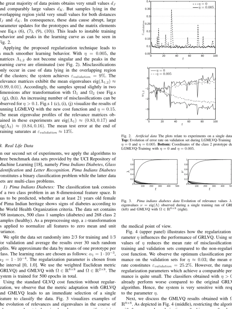
overlapping region yield very small values for both distances dJ and dK. In consequence, these data cause abrupt, large parameter updates for the prototypes and the matrix elements (see Eq.s (6), (7), (9), (10)). This leads to instable training behavior and peaks in the learning curve as can be seen in Fig. 2.
Applying the proposed regularization technique leads to
a much smoother learning behavior. With η = 0.005, the
matrices Λ1,2 do not become singular and the peaks in the learning curve are eliminated (see Fig. 2). Misclassifications only occur in case of data lying in the overlapping region of the clusters; the system achieves εvalidation = 9%. The relevance matrices exhibit the mean eigenvalues eig(Λ1,2)≈ (0.99,0.01). Accordingly, the samples spread slightly in two
dimensions after transformation with Ω1 and Ω2 (see Fig.s
1 (g), (h)). An increasing number of misclassifications can be observed forη >0.1. Fig.s 1 (c), (i), (j) visualize the results of
running LGMLVQ with the new cost function and η = 0.15.
The mean eigenvalue profiles of the relevance matrices ob-tained in these experiments are eig(Λ1) ≈ (0.83,0.17) and eig(Λ2) ≈ (0.84,0.16). The mean test error at the end of training saturates at εvalidation≈13%.
B. Real Life Data
In our second set of experiments, we apply the algorithms to three benchmark data sets provided by the UCI Repository of Machine Learning [18], namely Pima Indians Diabetes, Glass
Identification and Letter Recognition. Pima Indians Diabetes
constitutes a binary classification problem while the latter data sets are multi-class problems.
1) Pima Indians Diabetes: The classification task consists
of a two class problem in an 8-dimensional feature space. It has to be predicted, whether an at least 21 years old female of Pima Indian heritage shows signs of diabetes according to the World Health Organization criteria. The data set contains 768 instances, 500 class 1 samples (diabetes) and 268 class 2 samples (healthy). As a preprocessing step, az-transformation is applied to normalize all features to zero mean and unit variance.
We split the data set randomly into 2/3 for training and 1/3 for validation and average the results over 30 such random splits. We approximate the data by means of one prototype per class. The learning rates are chosen as follows:α1= 1·10−3, α2 = 1·10−4. The regularization parameter is chosen from the interval [0, 1.0]. We use the weighted Euclidean metric
(GRLVQ) and GMLVQ with Ω∈R8×8 and Ω∈R2×8. The
system is trained for 500 epochs in total.
Using the standard GLVQ cost function without regular-ization, we observe that the metric adaptation with GRLVQ and GMLVQ leads to an immediate selection of a single feature to classify the data. Fig. 3 visualizes examples of the evolution of relevances and eigenvalues in the course of relevance and matrix learning based on one specific training set. GRLVQ bases the classification on feature 2: plasma glucose concentration, which is also a plausible result from
0 20 40 60 80 100 0.05 0.1 0.15 0.2 0.25 0.3 0.35 0.4 t εv a li d a ti o n η= 0 η= 0.005 0 20 40 60 80 100 −4 −3 −2 −1 0 1 t w1 , 2 η= 0 η= 0.005
Fig. 2. Artificial data The plots relate to experiments on a single data set.
Top: Evolution of error rate on validation set during LGMLVQ-Training with η= 0andη= 0.005. Bottom: Coordinates of the class 2 prototype during LGMLVQ-Training withη= 0andη= 0.005.
100 200 300 400 500 0 0.2 0.4 0.6 0.8 1 t λ 100 200 300 400 500 0 0.2 0.4 0.6 0.8 1 t ν
Fig. 3. Pima indians diabetes data Evolution of relevance values λand eigenvalues ν =eig(Λ) observed during a single training run of GRLVQ (left) and GMLVQ withΩ∈R8×8
(right).
the medical point of view.
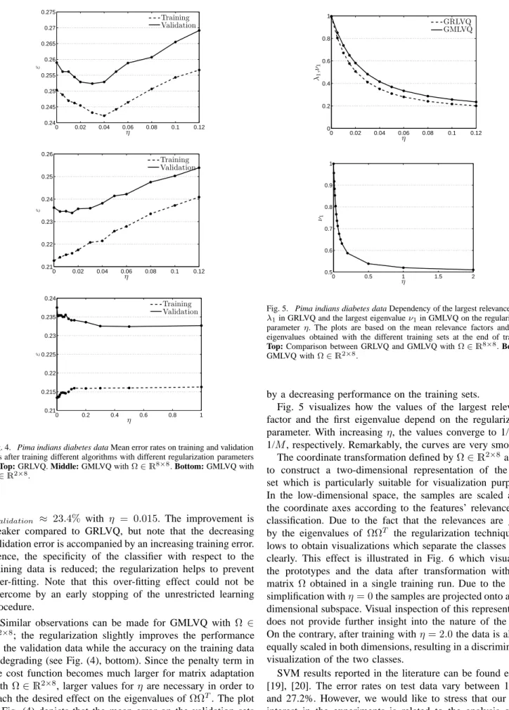
Fig. 4 (upper panel) illustrates how the regularization
pa-rameterηinfluences the performance of GRLVQ. Using small
values of η reduces the mean rate of misclassification on
training and validation sets compared to the non-regularized cost function. We observe the optimum classification perfor-mance on the validation sets for η ≈ 0.03; the mean error rate constitutes εvalidation = 25.2%. However, the range of regularization parameters which achieve a comparable perfor-mance is quite small. The classifiers obtained withη >0.06
already perform worse compared to the original GRLVQ-algorithm. Hence, the system is very sensitive with respect to the parameterη.
Next, we discuss the GMLVQ results obtained with Ω ∈
R8×8. As depicted in Fig. 4 (middle), restricting the algorithm with the proposed regularization method improves the classifi-cation of the validation data slightly; the mean performance on the validation sets increases for small values ofηand reaches
0 0.02 0.04 0.06 0.08 0.1 0.12 0.24 0.245 0.25 0.255 0.26 0.265 0.27 0.275 η ε Training Validation 0 0.02 0.04 0.06 0.08 0.1 0.12 0.21 0.22 0.23 0.24 0.25 0.26 η ε Training Validation 0 0.2 0.4 0.6 0.8 1 0.21 0.215 0.22 0.225 0.23 0.235 0.24 η ε Training Validation
Fig. 4. Pima indians diabetes data Mean error rates on training and validation sets after training different algorithms with different regularization parameters
η. Top: GRLVQ. Middle: GMLVQ withΩ∈R8×8
. Bottom: GMLVQ with
Ω∈R2×8.
εvalidation ≈ 23.4% with η = 0.015. The improvement is
weaker compared to GRLVQ, but note that the decreasing validation error is accompanied by an increasing training error. Hence, the specificity of the classifier with respect to the training data is reduced; the regularization helps to prevent over-fitting. Note that this over-fitting effect could not be overcome by an early stopping of the unrestricted learning procedure.
Similar observations can be made for GMLVQ with Ω ∈
R2×8; the regularization slightly improves the performance on the validation data while the accuracy on the training data is degrading (see Fig. (4), bottom). Since the penalty term in the cost function becomes much larger for matrix adaptation withΩ∈R2×8, larger values forη are necessary in order to reach the desired effect on the eigenvalues ofΩΩT. The plot in Fig. (4) depicts that the mean error on the validation sets reaches a stable optimum for η > 0.3; εvalidation = 23.3%. The increasing validation set performance is also accompanied
0 0.02 0.04 0.06 0.08 0.1 0.12 0 0.2 0.4 0.6 0.8 1 η λ1 , ν1 GRLVQ GMLVQ 0 0.5 1 1.5 2 0.5 0.6 0.7 0.8 0.9 1 η ν1
Fig. 5. Pima indians diabetes data Dependency of the largest relevance value
λ1in GRLVQ and the largest eigenvalueν1in GMLVQ on the regularization parameter η. The plots are based on the mean relevance factors and mean eigenvalues obtained with the different training sets at the end of training.
Top: Comparison between GRLVQ and GMLVQ withΩ∈R8×8
. Bottom: GMLVQ withΩ∈R2×8
.
by a decreasing performance on the training sets.
Fig. 5 visualizes how the values of the largest relevance factor and the first eigenvalue depend on the regularization parameter. With increasing η, the values converge to 1/N or 1/M, respectively. Remarkably, the curves are very smooth.
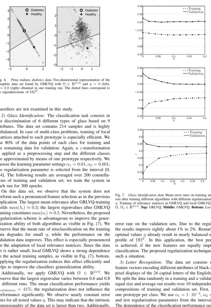
The coordinate transformation defined byΩ∈R2×8allows to construct a two-dimensional representation of the data set which is particularly suitable for visualization purposes. In the low-dimensional space, the samples are scaled along the coordinate axes according to the features’ relevances for classification. Due to the fact that the relevances are given
by the eigenvalues of ΩΩT the regularization technique
al-lows to obtain visualizations which separate the classes more clearly. This effect is illustrated in Fig. 6 which visualizes the prototypes and the data after transformation with one matrix Ω obtained in a single training run. Due to the over-simplification withη= 0the samples are projected onto a one-dimensional subspace. Visual inspection of this representation does not provide further insight into the nature of the data. On the contrary, after training withη= 2.0the data is almost equally scaled in both dimensions, resulting in a discriminative visualization of the two classes.
SVM results reported in the literature can be found e.g. in [19], [20]. The error rates on test data vary between 19.3% and 27.2%. However, we would like to stress that our main interest in the experiments is related to the analysis of the regularization approach in comparison to original GMLVQ. For this reason, further validation procedures to optimize the
−2 0 2 −3 −2 −1 0 1 2 3 Diabetes Healthy −2 −1 0 1 −3 −2 −1 0 1 2 Diabetes Healthy
Fig. 6. Pima indians diabetes data Two-dimensional representation of the
complete data set found by GMLVQ with Ω ∈ R2×8
and η = 0(left),
η= 2.0(right) obtained in one training run. The dotted lines correspond to the eigendirections ofΩΩT.
classifiers are not examined in this study.
2) Glass Identification: The classification task consists in
the discrimination of 6 different types of glass based on 9 attributes. The data set contains 214 samples and is highly unbalanced. In case of multi-class problems, training of local matrices attached to each prototype is especially efficient. We use 80% of the data points of each class for training and the remaining data for validation. Again, a z-transformation is applied as a preprocessing step and the different classes are approximated by means of one prototype respectively. We choose the learning parameter settingsα1= 0.01,α2= 0.001; the regularization parameter is selected from the interval [0, 0.4]. The following results are averaged over 200 constella-tions of training and validation set; we train the system in each run for 300 epochs.
On this data set, we observe that the system does not perform such a pronounced feature selection as in the previous application. The largest mean relevance after GRLVQ-training yields max(λi)≈0.3; the largest eigenvalues after GMLVQ training constitutesmax(νi)≈0.5. Nevertheless, the proposed regularization scheme is advantageous to improve the gener-alization ability of both algorithms as visible in Fig. (7). We observe that the mean rate of misclassification on the training
data degrades for small η, while the performance on the
validation data improves. This effect is especially pronounced for the adaptation of local relevance matrices. Since the data set is rather small, local GMLVQ shows a strong dependence on the actual training samples, as visible in Fig. (7), bottom. Applying the regularization reduces this effect efficiently and helps to improve the classifiers generalization ability.
Additionally, we apply GMLVQ with Ω ∈ R2×9. We
observe that the largest eigenvalue varies between 0.6 and 0.8 in different runs. The mean classification performance yields
εvalidation = 41%; the regularization does not influence the
performance significantly. We observe nearly constant error rates for all tested valuesη. This may indicate that the intrinsic dimensionality of the data set is larger than two. Additionally,
we ran the algorithm withM = 3andM = 4. WithM = 3we
achieve εvalidation ≈38.1%, M = 4 results in 37.2% mean
0 0.05 0.1 0.15 0.2 0.26 0.28 0.3 0.32 0.34 0.36 0.38 η ε Training Validation 0 0.05 0.1 0.15 0.2 0.26 0.28 0.3 0.32 0.34 0.36 0.38 η ε Training Validation 0 0.05 0.1 0.15 0.2 0.25 0.3 0.1 0.15 0.2 0.25 0.3 0.35 0.4 0.45 η ε Training Validation
Fig. 7. Glass identification data Mean error rates on training and validation
sets after training different algorithms with different regularization parameters
η. Training of relevance matrices in GMLVQ and local GMLVQ is based on
Ω,Ωj∈R9×9. Top: GRLVQ. Middle: GMLVQ. Bottom: Local GMLVQ.
error rate on the validation sets. Due to the regularization, the results improve sightly about 1% to 2%. Remarkably, the optimal valuesη already result in nearly balanced eigenvalue
profile of ΩΩT. In this application, the best performance
is achieved, if the new features are equally important for classification. The proposed regularization technique indicates such a situation.
3) Letter Recognition: The data set consists of 20 000
feature vectors encoding different attributes of black-and-white pixel displays of the 26 capital letters of the English alphabet. We split the data randomly in a training and a validation set of equal size and average our results over 10 independent random compositions of training and validation set. First, we adapt one prototype per class. We useα1= 1·10−3,α2= 1·10−4 and test regularization parameters from the interval [0, 0.1]. The dependence of the classification performance on the value of the regularization parameter for our GRLVQ and GMLVQ experiments are depicted in Fig. (8). It is clearly visible that
0 0.02 0.04 0.06 0.08 0.1 0.26 0.27 0.28 0.29 0.3 0.31 0.32 0.33 0.34 η ε Training Validation 0 0.02 0.04 0.06 0.08 0.1 0.26 0.27 0.28 0.29 0.3 0.31 0.32 0.33 0.34 η ε Training Validation 0 0.02 0.04 0.06 0.08 0.1 0.18 0.19 0.2 0.21 0.22 0.23 0.24 0.25 0.26 η ε Training Validation
Fig. 8. Letter recognition data set Mean error rates on training and validation sets after training different algorithms with different regularization parameters
η. Top: GRLVQ. Middle: GMLVQ withΩ ∈R16×16
. Bottom: GMLVQ withΩ ∈R16×16
and three prototypes per class.
the regularization improves the performance for small values ofη compared to the experiments with η= 0.
Compared to global GMLVQ, the adaptation of local rel-evance matrices improves the classification accuracy signifi-cantly; we obtainεvalidation ≈12%. Since no over-fitting or over-simplification effects are present in this application, the regularization does not achieve further improvements anymore. Additionally, we perform GMLVQ training with three pro-totypes per class. Slightly larger learning ratesα1= 5·10−3 andα2= 5·10−4 are used for these experiments in order to increase the speed of convergence; the system is trained for 500 epochs. Concerning the metric learning, the algorithm’s behavior resembles the previous experiments with only one prototype per class. This is depicted in Fig.s 8 and 9. Already small valuesη effect a significant reduction of the mean rate
of misclassification. Here, the optimal value η is the same
for both model settings. With η = 0.05, the classification
performance improves about≈2% compared to training with
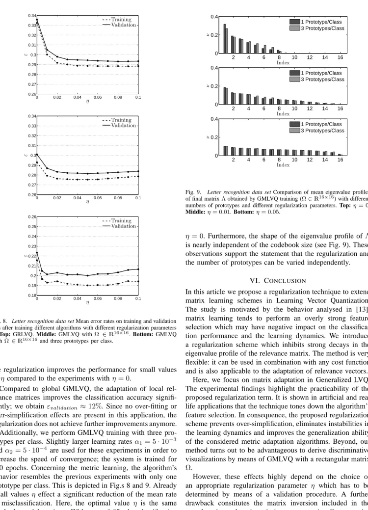
2 4 6 8 10 12 14 16 0 0.2 0.4 Index ν 1 Prototype/Class 3 Prototypes/Class 2 4 6 8 10 12 14 16 0 0.2 0.4 Index ν 1 Prototype/Class 3 Prototypes/Class 2 4 6 8 10 12 14 16 0 0.2 0.4 Index ν 1 Prototype/Class 3 Prototypes/Class
Fig. 9. Letter recognition data set Comparison of mean eigenvalue profiles
of final matrixΛobtained by GMLVQ training (Ω∈R16×16
) with different numbers of prototypes and different regularization parameters. Top:η= 0.
Middle:η= 0.01. Bottom:η= 0.05.
η = 0. Furthermore, the shape of the eigenvalue profile of Λ
is nearly independent of the codebook size (see Fig. 9). These observations support the statement that the regularization and the number of prototypes can be varied independently.
VI. CONCLUSION
In this article we propose a regularization technique to extend matrix learning schemes in Learning Vector Quantization. The study is motivated by the behavior analysed in [13]: matrix learning tends to perform an overly strong feature selection which may have negative impact on the classifica-tion performance and the learning dynamics. We introduce a regularization scheme which inhibits strong decays in the eigenvalue profile of the relevance matrix. The method is very flexible: it can be used in combination with any cost function and is also applicable to the adaptation of relevance vectors.
Here, we focus on matrix adaptation in Generalized LVQ. The experimental findings highlight the practicability of the proposed regularization term. It is shown in artificial and real life applications that the technique tones down the algorithm’s feature selection. In consequence, the proposed regularization scheme prevents over-simplification, eliminates instabilities in the learning dynamics and improves the generalization ability of the considered metric adaptation algorithms. Beyond, our method turns out to be advantageous to derive discriminative visualizations by means of GMLVQ with a rectangular matrix
Ω.
However, these effects highly depend on the choice of
an appropriate regularization parameter η which has to be
determined by means of a validation procedure. A further drawback constitutes the matrix inversion included in the new learning rules since it is a computationally expensive operation. Future projects will concern the application of the
regularization method on very high dimensional data. There, the computational costs of the matrix inversion can become problematic. However, efficient techniques for the iteration of an approximate pseudo-inverse can be developed which make the method also applicable for classification problems in high dimensional spaces.
REFERENCES
[1] T. Kohonen, Self-Organizing Maps, 2nd ed. Berlin, Heidelberg: Springer, 1997.
[2] V. Vapnik, The Nature of Statistical Learning Theory. New York, NY, USA: Springer, 1995.
[3] A. Sato and K. Yamada, “Generalized learning vector quantization,” in Advances in Neural Information Processing Systems 8. Proceedings
of the 1995 Conference, D. S. Touretzky, M. C. Mozer, and M. E.
Hasselmo, Eds. Cambridge, MA, USA: MIT Press, 1996, pp. 423– 9.
[4] S. Seo, M. Bode, and K. Obermayer, “Soft nearest prototype classifi-cation,” IEEE Transactions on Neural Networks, vol. 14, pp. 390–398, 2003.
[5] T. Bojer, B. Hammer, D. Schunk, and K. T. von Toschanowitz, “Rel-evance determination in learning vector quantization,” in European
Symposium on Artificial Neural Networks, M. Verleysen, Ed., Bruges,
Belgium, 2001, pp. 271–276.
[6] P. Schneider, M. Biehl, and B. Hammer, “Adaptive relevance matrices in learning vector quantization,” Neural Computation, vol. 21, no. 12, pp. 3532–3561, 2009.
[7] “Bibliography on the Self-Organizing Map (SOM) and Learning Vector
Quantization (LVQ),” Neural Networks Research Centre, Helskinki
University of Technology, 2002.
[8] A. Drimbarean and P. F. Whelan, “Experiments in colour texture analysis,” Pattern Recognition Letters, vol. 22, no. 10, pp. 1161–1167, 2001.
[9] B. Hammer and T. Villmann, “Generalized relevance learning vector quantization,” Neural Networks, vol. 15, no. 8-9, pp. 1059–1068, 2002. [10] M. Mendenhall and E. Mereyni, “Generalized relevance learning vector quantization for classification driven feature extraction from hyperspec-tral data,” in in Proc. ASPRS 2006 Annual Conference and Technology
Exhibition, 2006, p. 8.
[11] T. C. Kietzmann, S. Lange, and M. Riedmiller, “Incremental grlvq: Learning relevant features for 3d object recognition,” Neurocomputing, vol. 71, no. 13-15, pp. 2868–2879, 2008.
[12] P. Schneider, M. Biehl, and B. Hammer, “Distance learning in discrim-inative vector quantization,” Neural Computation, vol. 21, no. 10, pp. 2942–2969, 2009.
[13] M. Biehl, B. Hammer, F.-M. Schleif, P. Schneider, and T. Villmann, “Stationarity of relevance matrix learning vector quantization,” Univer-sity of Leipzig, Tech. Rep., 2009.
[14] S. Seo and K. Obermayer, “Soft learning vector quantization,” Neural
Computation, vol. 15, no. 7, pp. 1589–1604, 2003.
[15] K. Bunte, P. Schneider, B. Hammer, F.-M. Schleif, T. Villmann, and M. Biehl, “Limited rank matrix learning and discriminative visualiza-tion,” University of Leipzig, Tech. Rep. 03/2008, 2008.
[16] M. Biehl, R. Breitling, and Y. Li, “Analysis of tiling microarray data by learning vector quantization and relevance learning,” in International
Conference on Intelligent Data Engineering and Automated Learning.
Birmingham, UK: Springer LNCS, December 2007.
[17] K. B. Petersen and M. S. Pedersen, “The matrix cookbook,”
http://matrixcookbook.com, 2008.
[18] D. J. Newman, S. Hettich, C. L. Blake, and C. J. Merz, “Uci repository of machine learning databases,”
http://archive.ics.uci.edu/ml/, 1998.
[19] C. Ong, A. A. Smola, and R. Williamson, “Learning the kernel with hyperkernels,” Journal of Machine Learning Research, vol. 6, pp. 1043– 1071, 07 2005.
[20] H. Tamura and K. Tanno, “Midpoint-validation method for support vector machine classification,” IEICE - Trans. Inf. Syst., vol. E91-D, no. 7, pp. 2095–2098, 2008.