The Ramsey Steady State under Optimal Monetary
and Fiscal Policy for Small Open Economies
Angelo Marsiglia Fasolo
July, 2014
ISSN 1518-3548 CGC 00.038.166/0001-05
Working Paper Series
Edited by Research Department (Depep) – E-mail: workingpaper@bcb.gov.br
Editor: Francisco Marcos Rodrigues Figueiredo – E-mail: francisco-marcos.figueiredo@bcb.gov.br Editorial Assistant: Jane Sofia Moita – E-mail: jane.sofia@bcb.gov.br
Head of Research Department: Eduardo José Araújo Lima – E-mail: eduardo.lima@bcb.gov.br The Banco Central do Brasil Working Papers are all evaluated in double blind referee process. Reproduction is permitted only if source is stated as follows: Working Paper n. 357.
Authorized by Carlos Hamilton Vasconcelos Araújo, Deputy Governor for Economic Policy.
General Control of Publications
Banco Central do Brasil Comun/Dipiv/Coivi
SBS – Quadra 3 – Bloco B – Edifício-Sede – 14º andar Caixa Postal 8.670
70074-900 Brasília – DF – Brazil
Phones: +55 (61) 3414-3710 and 3414-3565 Fax: +55 (61) 3414-1898
E-mail: editor@bcb.gov.br
The views expressed in this work are those of the authors and do not necessarily reflect those of the Banco Central or its members.
Although these Working Papers often represent preliminary work, citation of source is required when used or reproduced.
As opiniões expressas neste trabalho são exclusivamente do(s) autor(es) e não refletem, necessariamente, a visão do Banco Central do Brasil.
Ainda que este artigo represente trabalho preliminar, é requerida a citação da fonte, mesmo quando reproduzido parcialmente.
Citizen Service Division
Banco Central do Brasil Deati/Diate
SBS – Quadra 3 – Bloco B – Edifício-Sede – 2º subsolo 70074-900 Brasília – DF – Brazil
Toll Free: 0800 9792345 Fax: +55 (61) 3414-2553
The Ramsey Steady State under Optimal Monetary and Fiscal
Policy for Small Open Economies
Angelo Marsiglia Fasolo
∗The Working Papers should not be reported as representing
the views of the Banco Central do Brasil. The views expressed in
the papers are those of the author and do not necessarily
reflect those of the Banco Central do Brasil.
Abstract
This paper describes the steady state allocations and prices for small open economies under optimal monetary and fiscal policy in a medium-scale DSGE model. The model encompasses the most common nominal and real rigidities normally found in the literature in a single framework. The Ramsey solution for the optimal monetary and fiscal policy is computed for a large space of the parameter set and for different combinations of fiscal policy instruments. Results show that, despite the large number of frictions in the model, optimal fiscal policy follows the usual results in the literature, with high taxes over labor income and low taxes (subsidies) on capital income. On the other hand, the choice of fiscal policy instruments is critical to characterize optimal monetary policy. Frictions associated with the small open economy framework do not play a critical role in characterizing the Ramsey planner’s policy choices.
JEL Codes: E52, E61, E63, F41, F42, F44
Keywords: Ramsey Policy; DSGE models; Small Open Economies; Monetary and Fiscal Policy
∗Research Department, Banco Central do Brasil. This paper is based on the dissertation written as a requirement to
a PhD degree at Duke University. The author would like to thank all the participants of seminars at Duke University and the Banco Central do Brasil and the Fulbright Commission and CAPES for financial support during the PhD pro-gram. This paper, however, does not necessarily represent the views and opinions of Banco Central do Brasil. E-mail: angelo.fasolo@bcb.gov.br
1
Introduction
What is the optimal combination of monetary and fiscal policy instruments for a small open economy? How does optimal policy changes when structural parameters characterize an emerging economy, in-stead of a developed economy? How do allocations and prices under optimal policy differ in a small open economy if the instrument set available for the benevolent planner changes? A lot of effort has been devoted to characterize optimal policy for developed small open economies, without discussing if the associated welfare ranking of policy recommendations is still the same for more volatile, less devel-oped economies. The high volatility observed in emerging economies usually translates in medium-scale dynamic stochastic general equilibrium (DSGE) models to parameter values far from those estimated to developed economies. This paper describes the allocations under optimal policy of a conventional medium-scale model for small open economies. In this paper, the main differences between Emerging Economies (EMEs, henceforth) and developed, Small Open Economies (SOEs, henceforth) will be re-stricted to structural parameters characterizing each economy. The exercise here focus on the description of the Ramsey policy steady state, clarifying the trade-offs faced by a benevolent central planner.
The development of DSGE models for closed economies1, comprising a large set of nominal and real
rigidities, changed research on optimal monetary and fiscal policies, not only because of the departure from analytically solving Ramsey’s (1927)[33] problem in tractable models, but also from a theoretical point of view. Models with such large number of frictions demand an equally large number of non-distortionary instruments in order to recover the first-best allocation as the equilibrium outcome of the optimal policy. In a framework constrained by the lack of such large set of instruments, the literature focused on the numerical characterization of the optimal policy’s outcome in models where the steady state is distorted as a consequence of the nominal and real rigidities. In these simulations, the government chooses values for a set of instruments in order to maximize (minimize) an utility (loss) function.
Few authors in the literature provide a comprehensive discussion about the properties of the steady state under the Ramsey policy. Woodford (2003)[43] provides a complete description of the steady state policy of the basic New Keynesian model for closed economies. The author explores differences in the Ramsey policy outcome when imposing additional restrictions like those included here, as the “timeless perspective” of the optimal policy problem. Still in the closed economy framework, but now dealing with variations of models similar in structure to Christiano, Eichenbaum and Evans (CEE, henceforth) (2005)[11], Schmitt-Groh´e and Uribe (SGU, henceforth) (2005, 2006, 2007)[36] [37] [38] explore the properties of the steady state under Ramsey optimal monetary and fiscal policies. These medium-scale models do not have a closed form solution, like the basic structures described in Woodford (2003)[43]. Therefore, the only way to understand and describe optimal policy is by means of numerical simulations. The results in terms of steady state of prices usually point out for price stability as the main outcome of the Ramsey planner, with small variations depending on the number of nominal and real rigidities included in the model.
Despite the adoption of medium-scale models for monetary policy analysis in some Central Banks, the research on optimal policy for SOEs in these models is still very incipient. The main focus of the literature is on the evaluation of optimal monetary policy in models with small departures from the basic sticky price framework proposed in Gal´ı and Monacelli (2005)[20] and Monacelli (2005)[32]. Extensions try to deal with specific features of open economies: deviations from the Law of One Price (Kollmann (2002)[25], Ambler, Dib and Rebei (2004)[5]); incomplete foreign asset markets (Ambler, Dib and Rebei (2004)[5], Justiniano and Preston (2009)[24]); fiscal policy dimension of the open economy framework (Benigno and De Paoli (2009)[8]). In the literature, no distinctions are made between SOEs
1The models are usually some variation of the framework in Christiano, Eichenbaum and Evans (2005)[11]. See
and EMEs, resulting in the same policy recommendations for both types of countries despite large differences documented in the literature between their structural parameters2.
The literature on EMEs focus on the description of these economies, adding structure over a basic model in order to capture distinctive aspects of data. The higher volatility in data, when compared with SOEs3, brings attention to topics like: foreign currency demand (Felices and Tuesta (2007)[19]);
investment financed by foreign currency and “balance sheet effects” (Devereux, Lane and Xu (2006)[17] and Elekdag and Tchakarov (2007)[18], Batini, Levine and Pearlman (2009)[7]); a commodity sector, in order to highlight the importance of natural resources (Laxton and Pesenti (2003)[26], Batini, Levine and Pearlman (2009)[7]); households heterogeneity in credit market access (Batini, Levine and Pearlman (2009)[7]). Most of these papers focus on the computation of optimal monetary policy rules, with little focus on fiscal policy or the structural parameters4, or, sometimes, assuming a steady state that might be different from the Ramsey optimal solution. Among the papers in this non-exhaustive list, Batini, Levine and Pearlman (2009)[7] is the closest reference in terms of the theoretical framework adopted here, as they compute optimal monetary and fiscal policy rules in a model with several nominal and real rigidities. However, the flexible price allocation can always be recovered as an optimal outcome of the policy due to the assumption of a lump sum taxation as one of the fiscal policy instruments.
From a theoretical perspective, the model here departs from the literature as it does not consider a set of lump sum mechanisms in order to eliminate the distortions caused by nominal rigidities: the Ramsey planner has access to distortionary consumption, capital and labor income taxes, besides the control of money supply and debt to balance the budget. As a consequence, the optimal policy allocations are not necessarily equivalent to those under flexible prices, just like the case for closed economies described in SGU (2005 and 2006)[36][37]. The computation of optimal policy is based on the solution for the Ramsey problem, where a planner tries to maximize the discounted expected utility of the representative household. This approach differs from other studies where optimal policy is derived from the minimization of an arbitrary loss function as a measure of welfare5. The steady state under optimal policy here is characterized under the same theoretical model, but fully exploring changes in parameter space, fiscal policy framework and nominal rigidities – in this case, rigidities located not only in domestic markets, but also in the price-setting mechanism of imported and exported goods.
One might ask about the importance of generalizing result on optimal policy under commitment for EMEs, given the high volatility and structural changes characterizing these economies. In reality, most of fiscal and monetary policy settings in EMEs are characterized by some type of commitment. The adoption of controlled exchange rate regimes in the early 90’s is an explicit commitment to keep exchange rate fluctuations under constraint. In the early 2000’s, several EMEs adopted a combination of high fiscal surpluses and inflation targeting regimes, while showing signs that little interference will be made in the exchange rate markets – again, a new form of commitment. Even in abnormal periods, like “sudden stops” episodes, governments usually sign “letters of intentions” to institutions like the IMF, committing to a new macroeconomic arrangement in order to guarantee emergency loans. Thus, the policy problem of EMEs can be viewed as setting the right commitment for these economies, instead of a proposition between commitment versus “discretionary policies”.
In terms of results, price stability seems to be the main goal of the Ramsey planner, given parameters
2Silveira (2006)[15] estimated the basic Gal´ı and Monacelli (2005)[20] model using Brazilian data. The posterior values
for the elasticity of the labor supply and the elasticity of substitution between imported and domestically produced consumption goods are outside the boundaries found in the literature. Another example is Elekdag, Justiniano and Tchakarov (2005)[41], with discrepancies in the values for the intertemporal elasticity of substitution and on the elasticity of the labor supply, when compared to the calibration used for closed economies.
3See Aguiar and Gopinath (2007)[3].
4There is an effort to put these models in an estimated framework. As an example, Elekdag, Justiniano and Tchakarov
(2005)[41] present an estimation of the model published later in Elekdag and Tchakarov (2007)[18].
5Some examples of the loss function approach are found in Svensson (2000)[40], Levin and Williams (2003)[27], Laxton
used in calibration. However, the number of available taxes for the government plays a key role in setting the optimal taxes and interest rates under different assumptions on nominal and real rigidities. To be more specific, the inclusion of consumption taxes as one of the taxes available in the model usually results in price stability as the optimal outcome, eliminating almost all trade-offs related to the combination of nominal and real rigidities. This result confirms, for a model designed for small open economies, the propositions in Correia, Nicolini and Teles (2008)[14] regarding the role of a tax over the final good of the economy, vis-a-vis a tax over intermediate inputs. The classical result from Judd (2002)[23], of a high subsidy to capital relative to the returns of labor, is robust for fiscal policy, irrespective to the set of instruments available to the benevolent government.
This paper is organized as follows. Chapter 2 presents the DSGE model, with focus on the equations characterizing the equilibrium and the connections between the structural frictions and the literature on DSGE models, finishing with the definitions of the competitive and the Ramsey equilibria. Chapter 3 shows the baseline calibration of the model. Chapter 4 presents a detailed analysis of the steady state of the model, assuming structural parameters normally observed in the literature. Chapter 5 concludes.
2
A Medium-Scale Model for Small Open Economies
In this section, a brief description of the model is provided with the characterization of the household and the firms’ problem, the policy rules for the government in a competitive equilibrium, the foreign sector and aggregation6. After that, the definitions of both a competitive and Ramsey equilibria are presented.
The model is an extension for a small open economy of the closed economy model for monetary policy analysis proposed in CEE (2005)[11] and Altig, Christiano, Eichenbaun and Lind´e (2005)[4]. Similar models are used in Adolfson, Lase´en, Lind´e and Villani (2007)[2] and in Christiano, Trabandt and Walentin (2007)[12]. These models combine the sticky price framework of Gal´ı and Monacelli (2005)[20] and Monacelli (2005)[32] to add nominal and real frictions based in CEE (2005)[11].
From the households’ perspective, the model presents external habit persistence in consumption, adjustment costs for investment, portfolio and capital utilization. Households’ objective is to maximize the discounted value of expected utility. They own capital, demand money to buy consumption goods and set wages after observing the demand for his specific type of labor. Households in each period buy both domestically produced and imported goods for consumption, sell labor to satisfy the demand by firms after the acceptance of the proposed wage and set the rate of capital utilization. In order to transfer wealth across periods, households trade bonds domestically and in international markets and accumulate capital built from both domestically produced and imported goods. They also face a cash-in-advance constraint, requiring domestic currency to buy a share of total consumption goods.
Firms in the tradable and non-tradable sectors of the domestic economy rent capital and labor from households to produce goods. They set prices in a Calvo style, with an exogenous probability of optimizing prices in period t.Firms from the tradable sector have to compete with imported goods retailers. These retail firms buy goods produced abroad and sell them domestically, also adjusting prices in domestic currency in a Calvo style. Also, firms from the tradable sector can sell goods for the exported goods retailers. These firms buy domestically produced goods and sell them abroad, setting price in foreign currency in a Calvo style – thus, local currency pricing in both domestic and foreign markets justifies pricing-to-market discrimination, as commonly seen in the literature7. A demand for
foreign currency is justified by a working capital constraint for imported goods retailers, with those firms selling bonds to obtain foreign currency to finance the acquisition of foreign inputs.
6Appendix A lists the final set of equilibrium conditions.
7Some models with at least partial local currency pricing are Kollmann (2002)[25], Ambler, Dib and Rebei (2004)[5],
The government in a competitive equilibrium sets nominal interest rates according to a Taylor rule based on current inflation, in order to match an exogenous, time-varying inflation target. In terms of fiscal policy, the government has three instruments available to finance an exogenous stream of consumption: money, bonds sold domestically, and distortionary taxes. The government might tax in different rates consumption and the income from capital, labor and profits. In the competitive equilibrium, taxes on labor are set according to a simple policy rule based on total government liabilities. Taxes on consumption, capital and on profits, as well as government spending, are exogenous.
The foreign sector is described by a VAR including the foreign currency supply, output, inflation, interest rates and the risk premium. The model has 16 shocks, with five from the foreign sector, plus the following: one on the price of imported goods in foreign currency; two stationary sectorial productiv-ity shocks; a non-stationary aggregate productivproductiv-ity shock; a non-stationary, investment-specific shock; government spending; three tax shocks; monetary policy shock and a inflation target shock.
2.1
Households
There is a continuum of infinitely-lived householdsi(i∈[0,1]) populating the domestic economy, each of them with an endowment of labor typei, ht(i). There is no population growth and labor can not be sold for firms in the rest of the world. In the intertemporal problem, households maximize discounted utility choosing consumption, capital utilization and investment for each sector, wages, hours worked and setting the money demand, next period’s foreign and domestic bond holdings and physical capital stock. The general intertemporal household problem, given the non-Ponzi games constraints, is:
maxE0 ∞ X t=0 βt[(1−γ) log (Ct(i)−ζCt−1) +γlog (1−ht(i))] s.t.: Pt(1 +τtc)Ct(i) + Υ−t1Pt Ix,td (i) +I d n,t(i) +PtMt(i) +Rt−1Bh,t(i) +StRft−1IBt(i) +Wtφ2w W t(i) πχwt Wt−1(i)−µ I2+ψ1 2 Yt B h,t+1(i) Yt − Bh Y 2 +ψ2 2Yt S tIBt+1(i) PtYt − rer IB Y 2 =Pt−1Mt−1(i) + 1−τth Wt(i)ht(i) +1−τtφPtΦt(i) + 1−τtk Pt Rn,tk µn,t−Υ−t1a(µn,t) Kn,t(i) + Rkx,tµx,t−Υ−t1a(µx,t) Kx,t(i) +Bh,t+1(i) +StIBt+1(i) Kj,t+1(i) = (1−δ)Kj,t(i) +Ij,td (i) 1− ℵ Id j,t(i) Id j,t−1(i) !! a(µj,t) =θ1(µj,t−1) + θ2 2 (µj,t−1) 2 Kj,t=µj,tKj,t ℵ Id i,t Id i,t−1 = φi 2 Id i,t Id i,t−1 −µI 2 j={x, n} Υt+1 Υt =µΥt+1= (1−ρΥ)µΥ+ρΥµΥt + Υ t+1; Υ t ∼N(0, σΥ) ht(i) = Wt(i) Wt −$ ht Mt(i)≥νm(1 +τtc)Ct(i)
In this problem,β is the intertemporal discount factor of the utility function. The utility function is log-separable in terms of consumption and labor, with consumption adjusted by external habit persistence8.
The degree of habit persistence is defined by the parameterζ∈[0,1).
Households accumulate physical capital,Kj,t, forj={x, n}representing the sectors of the economy, buying from the firms investment goods that depreciate at a rateδ. Define Υ−t1 as the non-stationary inverse of the relative price of investment in terms of consumption goods. The relative price of investment goods can also be interpreted as a technology shock affecting the linear production function available to households to transform consumption goods in investment goods9. Investment is subject to an adjustment
costℵ(.),in the same fashion as in CEE (2005)[11] and Altig, Christiano, Eichenbaun and Linde (2005)[4] such thatℵ(1) = 0,ℵ0(1) = 0,ℵ00(1)>0.10The functional form follows SGU (2006)[37], withµIdefining the steady state growth of investment. Households rent capital for firms after setting the rate of capital utilization for each sector (µj,t), paying a cost given by a(µj,t) to change the utilization level in each period and in each sector. The after-tax private return of capital in each sector is defined, thus, as
1−τk t
Pt Rkj,tµj,t−Υt−1a(µj,t)Kj,t(i).
The supply of labor is decided by each household taking as given the aggregate wage and demand for labor of the economy, Wt andht,and the adjustment cost for wages. As a monopolist of a specific type of labor, household chooses the nominal wageW(i) and supplies all the demanded laborht(i) given the acceptance ofW(i).The elasticity of substitution across different types of labor is given by $ >1. The nominal wage adjustment cost function allows for partial indexation based on current inflation, determined byχw(χw∈[0,1]). The presence of sticky wages results in an additional distortion, defined bymcwt, which is the markup imposed over real wages as households supply a specific type of labor. The quadratic adjustment cost11is consistent with the absence of lump sum instruments to correct for wealth
dispersion across households. Wage-setting processes based on Calvo model create dispersion in wage income across households, with the representative household recovered by lump sum subsidy schemes or an asset market structure capable of insuring households against wage dispersion. Both instruments would be controversial with the evaluation of optimal policy assuming that government does access lump sum schemes to support agents. Another alternative is to assume a centralized union coordinating the supply of labor, as in SGU (2006)[37]. The assumption of a labor union with such market power, however, does not seem reasonable for developed small open economies outside a few European countries12.
Still in the budget constraint, households allocate wealth over time buying one-period, non-state contingent nominal bonds from the government,Bh,t+1(i), or from the rest of the world,IBt+1(i).In the
later case, bonds are priced in foreign currency, andSt is the nominal exchange rate. In order to adjust portfolio, and to induce stationarity in the model, households incurs in costs based on the variance of the stock of bonds as a proportion of the GDP13. Households also receive dividends from firms Φ
t(i). Finally, following SGU (2007)[38], households demand money, Mt(i) in order to pay for a share νm≥0 of consumption. The sequence of events in each period is the same as in CEE (2005)[11], with the households first deciding consumption and capital allocation, then deciding, in sequence, the financial portfolio, wages and the labor supply, and the final composition of portfolio between bonds and money.
8In terms of notation, the general variablex
t(i) represents the choice of householdion periodtaboutx.The variable
xtis the aggregate value ofxt(i) for the economy.
9See Greenwood, Hercowitz and Krusell (2000)[22] and SGU (2006)[37].
10Adjustment costs and the structure of shocks, despite not affecting the deterministic steady state of the model, are
kept in the description of the model for the sake of completeness. It is left, also, as a suggested structure for reference in order to study the dynamic properties of the Ramsey equilibrium.
11See, for instance, Chugh (2006)[13] and Garc´ıa-Cicco (2009)[21].
12According to data from OECD (2004), only Denmark, Sweden, Finland, Iceland and Belgium presented a steady
increase in trade-union density from 1960 to 2000. In Latin American economies, the trade-union density is not only lower, compared to Scandinavian countries, but also declining since the 1990’s – see Visser Martin Tergeist, 2008[42].
13See SGU (2003b)[35]. The use of the ratio to GDP in the functional form adopted here makes it easier to obtain the
Thus, domestic currency is expressed as an end-of-period aggregate. Defineλet/Pt,eλtqej,t, λmt eλtand e λt 1−τth Wt
/(Ptmcwt) the Lagrange multipliers on the budget constraint, on the capital accumulation equations, on the cash-in-advance constraint and on the labor demand function, respectively. Noting that, in the symmetric equilibrium,Ct(i) =Ctand Wt(i) =Wt, the final set of equilibrium conditions of the intertemporal problem of households is given by:
1−τh t f Wt (1 +τc t) (Ct−ζCt−1) = γ (1−γ) mcwt 1 +νmRet−1 e Rt (1−ht) (1) (1−γ) Ct−ζCt−1 = (1 +τtc)eλt 1 +νm Rt−1 Rt (2) e λt 1−ψ1 B h,t+1 Yt −Bh Y =βRtEt e λt+1 πt+1 ! (3) e λt 1−ψ2 S tIBt+1 PtYt −rer IB Y =βRftEt S t+1 St Pt Pt+1 e λt+1 (4) e λtqex,t=βEt n e λt+1 1−τtk+1 Rx,tk +1µx,t+1−Υt−+11a(µx,t+1) +qex,t+1(1−δ) o (5) e λtqen,t=βEt n e λt+1 1−τtk+1 Rn,tk +1µn,t+1−Υt−+11a(µn,t+1) +qen,t+1(1−δ) o (6) Kn,t =µn,tKn,t (7) Kx,t=µx,tKx,t (8) θ1+θ2(µn,t−1) = Rk n,t Υ−t1 (9) θ1+θ2(µx,t−1) = Rkx,t Υ−t1 (10) Rt= 1 rt,t+1 (11) e Rt=Rt 1−ψ1 B h,t+1 Yt −Bh Y −1 (12) e λtΥ−t1 = eλtqex,t " 1−Ψ I d x,t Id x,t−1 ! − I d x,t Id x,t−1 ! Ψ0 I d x,t Id x,t−1 !# +βEt eλt+1qex,t+1 Id x,t+1 Id x,t !2 Ψ0 I d x,t+1 Id x,t ! (13) e λtΥ−t1 = eλtqen,t " 1−Ψ I d n,t Id n,t−1 ! − I d n,t Id n,t−1 ! Ψ0 I d n,t Id n,t−1 !# +βEt eλt+1eqn,t+1 In,td +1 Id n,t !2 Ψ0 I d n,t+1 Id n,t ! (14) Kx,t+1(i) = (1−δ)Kx,t(i) +Ix,td (i) 1− ℵ Id x,t(i) Id x,t−1(i) !! (15) Kn,t+1(i) = (1−δ)Kn,t(i) +In,td (i) 1− ℵ In,td (i) Id n,t−1(i) !! (16)
1−$ $ + 1 mcwt $ht 1−τth =− φw πχw−1 t f Wt f Wt−1 ! f Wt πχw−1 t Wft−1 −µI ! +βEt e λt+1φw e λtπ χw−1 t+1 f Wt+1 f Wt !2 f Wt+1 πχw−1 t+1 Wft −µI ! (17)
From the first order conditions, notice that the uncovered interest parity (UIP) condition between domestic and foreign interest rates can be recovered after linearizing equations 3 and 4. The UIP condition holds in its strict sense only in the steady state, since the non-linear dynamics is also influenced by the presence of domestic and foreign portfolio adjustment costs. This is a departure from other studies, like Adolfson, Lase´en, Lind´e and Villani (2007)[2], where the only source of discrepancy between the domestic and foreign interest rates from the UIP condition is the debt-elastic foreign interest rate. As the description of the foreign block of the model will make clear, the UIP condition combines the debt-elastic foreign interest rate and the portfolio adjustment cost proposed in SGU (2003b)[35].
The household also solves a sequence of minimization problems constrained by the CES function in order to choose the composition of the consumption and investment goods. Expressing first the consumption problem, households decide between imported and domestically produced goods in the tradable goods basket, and then chooses the optimal composition of tradable and non-tradable goods. For simplicity, assume that portfolio adjustment costs are paid with a share of the consumption goods acquired by the households. As a consequence, the cost minimization problem is given by:
min Cn,t,Ct,t,Cm,t,Cx,t Pn,tCn,t+Pt,tCt,t Ct+P ACb,t+P ACib,t= h (1−ω)1εC ε−1 ε n,t +ω 1 εC ε−1 ε t,t iε−ε1 (18) Ct,t= (1−κ) 1 %C %−1 % x,t +κ 1 %C %−1 % m,t %−%1 (19) P ACb,t= ψ1 2 Yt Bh,t+1 Yt −Bh Y 2 P ACib,t= ψ2 2 Yt S tIBt+1 PtYt −IB Y 2
Combine the first order conditions to obtain the demand for each type of tradable good:
Cm,t=κ P m,t Pt,t −% Ct,t (20) Cx,t= (1−κ) P x,t Pt,t −% Ct,t (21)
By analogy, the optimal decision between tradable and non-tradable goods is given by:
Ct,t=ω P t,t Pt −ε (Ct+P ACb,t+P ACib,t) (22) Cn,t = (1−ω) P n,t Pt −ε (Ct+P ACb,t+P ACib,t) (23)
Households solve a similar problem setting the investment good in each sector. For simplicity, assume that the weights and the elasticities of substitution among different investment goods are the same as those for consumption goods. Adjustment costs in capital utilization are paid in terms of
aggregate investment. The demand for home produced and imported investment goods become: Υ−t1It= Υ−t1 In,td +a(µn,t)Kn,t+Ix,td +a(µx,t)Kx,t (24) Im,t=κ P m,t Pt,t −% It,t (25) Ix,t= (1−κ) Px,t Pt,t −% It,t (26) It,t=ω Pt,t Pt −ε Υ−t1It (27) In,t = (1−ω) P n,t Pt −ε Υ−t1It (28)
2.2
Firms
There are four sectors in the economy, each sector composed by a continuum of firms in a monopolistic competitive framework. Firms in non-tradable (n) and tradable (x) sectors demand labor and capital to produce. Firms in the imported (exported) goods sector, m (xp), buy the final good and sell it in the domestic economy (rest of the world). Firms chooses the amount of input and set prices based on a probability αi, i={n, x, m, xp}, that is independent across sectors and firms. Firms not allowed to optimize prices in period t change prices according to an indexation rule based on past inflation. Imported goods’ firms must finance input acquisition using foreign currency. There is no firm entry into or exit out of sectori.Equations describing price dynamics would result, in a log-linearized model around price stability, in equations like the New Keynesian Phillips curve. However, since price stability might not be optimal for Ramsey planner, the recursive formulation for the first order condition in terms of prices described in SGU (2006)[37] is adopted.
2.2.1 Domestic non-tradable goods’ producers problem:
Firms in the non-tradable sector produce goods used for consumption, investment and spent by the government. Setting real profits as Φn,t(in), the problem of producers of typein product (in∈[0,1]) is to maximize the expected discounted stream of profits, subject to the demand for goodin,the production technology and the aggregate demand for non-tradable goods. Firms choose in each period the demand for labor, capital and, with probability 1−αn, they optimize prices. The problem is given by:
maxE0 ∞ X t=0 r0,tPn,t P n,t(in) Pn,t Dn,t(in)− Wt Pn,t hn,t(in)− Pt Pn,t Rkn,tKn,t(in) s.t.: Dn,t(in) = P n,t(in) Pn,t −ηn Yn,t Yn,t =Cn,t+Gn,t+ Υ−t1 Pt Pn,tIn,t an,tKn,t(in) θ (zthn,t(in)) 1−θ −zt∗χn≥Dn,t(in) Υ θ 1−θ t = z∗t zt zt+1 zt =µ z t+1= (1−ρz)µz+ρzµzt+tz+1; ρz∈[0,1) ; zt ∼N(0, σz) logan,t+1=ρnlogan,t+nt+1; ρn∈[0,1) ; nt ∼N(0, σn)
non-stationary technology shock, affecting firms using labor as input. In order to guarantee zero profits in the steady state,z∗tχn introduces a fixed cost proportional to the evolution of the non-stationary shock, following CEE (2005)[11] and SGU (2005, 2006)[36][37]. Parameter ηn is the elasticity of substitution across varieties of non-tradable goods.
From the first order conditions in terms of hn,t(in) and Kn,t(in), it is possible to prove that the capital-labor ratio and the marginal cost are the same across firms in the non-tradable sector. Setting mcn,t as the Lagrange multiplier on the firm’s demand constraint, the equilibrium conditions are:
f Wt Pt Pn,t =mcn,t(1−θ)an,tzt Kn,t zthn,t θ (29) Rkn,t Pt Pn,t =mcn,tθan,t K n,t zthn,t θ−1 (30)
Prices are formed in a Calvo style with indexation, whereαn is the probability that firm in is not allowed to optimally adjust its price in periodt.In the case firms are not allowed to optimize prices, they follow the rulePn,t(in) =πn,tκn−1Pn,t−1(in),for 0≤κn≤1 andπn,t+1=
Pn,t+1
Pn,t .Setting the Lagrangean
of the problem, considering only the relevant terms for price determination:
Ln =Et ∞ X s=0 αsnrt,t+sPn,t+s e Pn,t(in) Pn,t+s !1−ηn s Y k=1 πκn n,t+k−1 πn,t+k 1−ηn Yn,t+s −mcn,t+s e Pn,t(in) Pn,t+s !−ηn s Y k=1 πκn n,t+k−1 πn,t+k −ηn Yn,t+s
In this problem,rt,t+s is the stochastic discount factor between periodstandt+s, andPen,t(in) is the new price set by firms allowed to adjust prices in periodt. The first order condition for firms is:
Et ∞ X s=0 αsnrt,t+sYn,t+sPn,t+s e Pn,t(in) Pn,t+s !−ηn s Y k=1 πκn n,t+k−1 πn,t+k −ηn × (ηn−1) ηn e Pn,t(in) Pn,t+s s Y k=1 πκn n,t+k−1 πn,t+k −mcn,t+s ! = 0
Since markup over prices is the same across firms, the symmetric equilibrium is characterized by all firms in sector nallowed to adjust prices in period t setting the same price:Pen,t(in) =Pen,t. Following SGU (2006)[37], split the first order condition in two parts,X1
t andXt2, and definepen,t=
e Pn,t
Pn,t in order
to obtain a recursive solution for the price-setting problem:
Xt1=Yn,tpe −1−ηn n,t mcn,t+αnrt,t+1Et e pn,t e pn,t+1 −1−ηn πκn n,t π(1+ηn)/ηn n,t+1 !−ηn Xt1+1 (31) Xt2=Yn,tpe −ηn n,t (ηn−1) ηn +αnrt,t+1Et e pn,t e pn,t+1 −ηn πκn n,t πηn/(ηn−1) n,t+1 !1−ηn Xt2+1 (32) Xt1=Xt2 (33)
2.2.2 Tradable goods’ producers problem:
A tradable goods producerix(ix∈[0,1]) solves the same problem as the non-tradable producer, using labor and capital as production inputs. The production of the tradable good is divided between domestic
absorption (consumption, investment and government spending) and the demand of a continuum ofixp exporting firms (Dxp,t). The tradable goods’ firm problem is given by:
maxE0 ∞ X t=0 r0,tPx,t Px,t(ix) Px,t Dx,t(ix)− f Wt Px,t hx,t(ix)− Pt Px,t Rkx,tKx,t(ix) ! s.t.: Dx,t(ix) = P x,t(ix) Px,t −ηx Yx,t Yx,t=Cx,t+Gt,t+ Υ−t1 Pt Px,tIx,t+Dxp,t ax,tKx,t(ix) θ (zthx,t(ix)) 1−θ −z∗tχx≥Dx,t(itr) Υ θ 1−θ t = z∗t zt zt+1 zt =µ z t+1= (1−ρz)µz+ρzµzt+tz+1; ρz∈[0,1) ; zt ∼N(0, σz) logax,t+1=ρxlogax,t+xt+1; ρx∈[0,1) ; xt ∼N(0, σx)
χxis a fixed cost related to the non-stationary shock ensuring zero profits in steady state. Parameter ηxis the elasticity of substitution across types of tradable goods. Settingmcx,tas the Lagrange multiplier, the cost minimization problem, noting that capital-labor ratio is the same across firms, implies:
f Wt Pt Px,t =mcx,t(1−θ)ax,tzt K x,t zthx,t θ (34) Rkx,t Pt Px,t =mcx,tθax,t K x,t zthx,t θ−1 (35)
Similar to the non-tradable sector, price adjustment is based on a Calvo mechanism with indexation, with 0≤κx≤1 defining the degree of indexation in the tradable sector. Taking the first order conditions in terms ofPex,t(ix), and defining πx,t+1 =
Px,t+1
Px,t , the optimal price set by each firm solves a recursive
problem that can be split in two equations forZt1, Zt2,such thatZt1=Zt2, andpex,t=
e Px,t Px,t : Zt1=pe−1−ηx x,t Yx,tmcx,t+αxrt,t+1Et e px,t e px,t+1 −1−ηx πκx x,t π(1+ηx)/ηx x,t+1 !−ηx Zt1+1 (36) Zt2=pe−ηx x,t Yx,t (ηx−1) ηx +αxrt,t+1Et e px,t e px,t+1 −ηx πκx x,t πηx/(ηx−1) x,t+1 !1−ηx Zt2+1 (37) Zt1=Zt2 (38)
2.2.3 Imported goods’ firms problem:
Following Lubik and Schorfheide (2006)[29], deviations from the Law of One price arises as a consequence of price stickiness in imported and exported goods. An imported goods’ firm im (im ∈ [0,1]) buys a bundle of the international homogeneous good14 and label it as an imported good type im. In order to buy input from the rest of the world, the firm needs to pay using foreign currency. The firm sells intraperiod bonds in foreign markets in order to get foreign currency, but it does not transfer financial
14In the model, one country buys a combination of final goods from different countries, generating a gap between the
wealth over time. As a consequence, firms face only an increase in the marginal cost of production. As a timing convention, traded bonds do not reflect in the end of period balance of payments. The same framework is adopted in Christiano, Trabandt and Walentin (2007)[12] and Mendoza and Yue (2008)[31]. The budget constraint of the importing firmim,expressed in terms of domestic prices, is given by:
StPt∗ Pt Mm,t∗ (im) + St Pt B∗m,t+1(im) = St Pt Pt∗−1Mm,t∗ −1(im) + St Pt Rtf−1Bm,t∗ (im) + P m,t(im)−StPm,t∗ Pt Dm,t(im)−zt∗χm−Φm,t(im)
where χm is a fixed cost associated with the non-stationary shock in order to guarantee zero profits in steady state. Following assumptions that firms do not keep any financial wealth across periods and that all profits are distributed to the households, obtain the expression for real profits:
P∗ tMm,t∗ (im) +R f tBm,t∗ +1(im) = 0, ∀t =⇒Φm,t(im) = P m,t(im)−StPm,t∗ Pt Dm,t(im)−zt∗χm− StPt∗ Pt Rft −1 Rtf ! Mm,t∗ (im)
The imported goods’ firm problem becomes:
max e Pm,t(im) E0 ∞ X t=0 r0,t " Pm,t(im)−StPm,t∗ Pt Dm,t(im)−zt∗χm− StPm,t∗ Pt Rft −1 Rft ! Pt∗ Pm,t∗ M ∗ m,t(im) # s.t.:Dm,t(im) = P m,t(im) Pm,t −ηm Cm,t+ Υ−t1 Pt Pm,t Im,t Mm,t(im)≥ Pm,t∗ Pt∗ Dm,t(im)
wherePm,t∗ is the price of the imported good bought by the domestic economy, quoted in foreign prices. Defineηmas the elasticity of substitution across varieties of imported goods,αmas the probability that firm im is not allowed to adjust prices in period t, πm,t+1 =
Pm,t+1
Pm,t and 0 ≤ κm ≤ 1 the degree of
indexation in the imported goods’ sector. Taking the first order conditions in terms of Pem,t(im), and as a consequence of the same mark-up over prices across firms (given by the real exchange rate based on the import price level), the symmetric equilibrium is characterized byPem,t(im) =Pem,t. The recursive solution for the problem is obtained after definingY1
t andYt2 such thatYt1=Yt2, and epm,t=
e Pm,t Pm,t : Yt1=ep−1−ηm m,t Cm,t+ Υ−t1Pt Pm,t Im,t S tPm,t∗ Pm,t 1 + R f t −1 Rft ! +αmrt,t+1Et e pm,t e pm,t+1 −1−ηm πκm m,t π(1+ηm)/ηm m,t+1 !−ηm Yt1+1 (39) Yt2=ep−ηm m,t Cm,t+ Υ−t1Pt Pm,t Im,t (η m−1) ηm +αmrt,t+1Et e pm,t e pm,t+1 −ηm πκm m,t πηm/(ηm−1) m,t+1 !1−ηm Yt2+1 (40) Yt1=Yt2 (41)
2.2.4 Exported goods’ firms problem:
An exported goods’ firmixp(ixp∈[0,1]) buys a share of the final tradable good in the domestic economy and sell it to the rest of the world, setting prices in foreign currency in a Calvo style – thus, prices are
sticky in foreign currency. The firm problem is given by: max e P∗ x,t(ixp) E0 ∞ X t=0 r0,t " StPex,t∗ (ixp)−Px,t Pt ! Dxp,t(ixp)− R t−1 Rt Mxp,t(ixp)−zt∗χxp # s.t.:Dxp,t(ixp) = P∗ x,t(ixp) Px,t∗ −ηxp Xt
where χxp is a fixed cost associated with the non-stationary shock in order to guarantee zero profits in steady state. Define ηxp as the foreign elasticity of substitution across varieties of domestic exported goods,π∗x,t+1=
Px,t∗ +1 P∗
x,t , 0≤κxp≤1 as the degree of indexation in the exported goods’ sector,αxpas the
probability that firmixis not allowed to optimize prices in periodt,andPx,t∗ as the price of the tradable good quoted in foreign currency. Taking first order conditions in terms ofPex,t∗ (ixp), and given that the symmetric equilibrium is characterized byPex,t∗ (ix) =Pex,t∗ ,the recursive solution for the pricing problem
of the exporting firms is obtained after properly definingU1
t andUt2 andpe ∗ x,t= e P∗ x,t P∗ x,t : Ut1= pe ∗ x,t −1−ηxp Xt Px,t StPx,t∗ +αxprt,t+1Et e p∗x,t e p∗x,t+1 !−1−ηxp π∗x,tκxp π∗x,t+1 (1+ηxp) ηxp −ηxp Ut1+1 (42) Ut2= pe ∗ x,t −ηxp Xt (ηxp−1) ηxp +αxprt,t+1Et e p∗x,t e p∗x,t+1 !−ηxp π∗x,tκxp π∗ x,t+1 (ηxpηxp−1) 1−ηxp Ut2+1 (43) Ut1=Ut2 (44)
2.3
Government
In a competitive equilibrium, the government follows simple rules to set monetary and fiscal policy. For the sake of this paper, as the steady state of the model is not affected by interest rate rules, assume that the government follows a standard Taylor rule, based on the deviations of inflation from an exogenous, autocorrelated inflation target and an autoregressive component15:
log R t+1 R =ρRlog R t R +απlog π t+1 πo t+1 +Rt+1; Rt ∼N(0, σR) (45) πot+1= (1−ρπo)πo+ρπoπot+π o t+1; πo t ∼N(0, σπo) (46)
The government, in order to finance its exogenous expenditures,Gt, collects distortionary taxes on consumption, labor, capital and profits income (τc
t, τth, τtk and τ φ
t), sells bonds domestically, Bg,t and controls the money supply,Mt. The government budget constraint is given by:
PtGt+Rt−1Bg,t=PtTt+PtMt+Bg,t+1−Pt−1Mt−1 Gt=zt∗gt gt= (1−ρg)g+ρggt−1+ g t; g t ∼N(0, σg) (47) Tt=τtcCt+τthWftht+τ φ tΦt+τtk Rkn,tµn,t−Υ−t1a(µn,t) Kn,t+ Rkx,tµx,t−Υ−t1a(µx,t) Kx,t (48) Rewriting the government budget constraint as a function of total real government liabilities (Lt):
Lt−1≡Mt−1+
Rt−1
Pt−1
Bg,t (49)
15To be more specific, any Taylor rule that ensures a non-zero, stationary inflation around the steady state satisfy the
=⇒Lt= Rt
πt
Lt−1+Rt(Gt−Tt)−(Rt−1)Mt (50) To close the dynamics of fiscal policy, assume that government follows a policy rule for labor income taxation based on real liabilities as a function of GDP and the output gap. Taxes on capital and profits are exogenous. The assumption of a policy rule for labor income taxes is an arbitrary choice that does not affect the steady state of the model. For simplicity, assume also that taxation on profits is constant over time. Notice that taxes on profits are lump sum transfers from households to the government. In this sense, it does not interfere with dynamics under the competitive equilibrium, where profits are zero.
τth−τh=ψli L t Yt − l y +ψy(yt−y) +τ ht ; τ h t ∼N(0, στ h) (51) τtk = (1−ρτ k)τk+ρτ kτtk−1+ τ k t ; τ k t ∼N(0, στ k) (52) τtφ=τφ (53) τtc= (1−ρc)τc+ρcτtc−1+ τ c t ; τ c t ∼N(0, σc) (54)
Additionally, the government solves the same problem as households to determine the consumption of tradable and non-tradable goods. By assumption, the government does not consume imported goods16:
Gn,t= (1−ω) P n,t Pt −ε Gt (55) Gt,t=ω Pt,t Pt −ε Gt (56)
2.4
International Financial Markets and World’s Economy
The transmission of shocks from international financial markets assumes a market capable of pricing country-specific risk on bonds traded outside domestic economy. A mechanism to induce stationarity as in SGU (2003b)[35] is used to determine the risk premium of bonds as a function of the net foreign position of the economy. The international interest rate is given by:
Rft =R∗t(1 +ξt) κ1 StIBt+1 PtYt /IB Y κ2 (57)
In this equation,R∗t is the nominal interest rate on a risk-free bond;ξtis an exogenous shock with expected value equal to the long run risk premium of the domestic economy,ξ∗; the last term is the gap of external debt as a proportion of GDP.
The world’s economy is set as a stationary VAR with output, y∗t, inflation,π∗t, interest rates,R∗t, growth of money supply, ∆Mt∗, and the risk premium,ξt, providing five shocks for the model. As the VAR does not influence the steady state, it is not necessary to be more specific with respect to additional structure. In the system,Ais a 5 by 5 matrix of coefficients, P
is a 5 by 5 covariance matrix of shocks.
∆Mt∗ ∆M∗ ξt ξ∗ R∗t R∗ πt∗ π∗ y∗ t y∗ =A ∆Mt∗−1 ∆M∗ ξt−1 ξ∗ Rt∗−1 R∗ πt∗−1 π∗ y∗ t−1 y∗ + m∗ t ξt R∗ t π∗ t yt∗ m∗ t ξt R∗ t π∗ t yt∗ iid ∼(0,P) (58)
Two assumptions close the link between prices and quantities of goods between the domestic econ-omy and the rest of world. First, assume that foreign households solve an expenditure minimization
problem to set the demand for home produced tradable goods. The solution of this problem is given by: Xt= P∗ x,t Pt∗ −η∗ z∗ty∗t (59)
Finally, the terms of trade are defined as the ratio between the exported goods and the imported goods price levels, both in foreign currency. The dynamics of the price of imported goods is given by an error-correction model that ensure the terms of trade becomes stationary, as in Garc´ıa-Cicco (2009)[21]:
tott= πx,t∗ π∗ m,t tott−1 (60) πtm∗ πm∗ =υ1 πm∗ t−1 πm∗ +υ2tottott−1 +§Xt∗−1+πmt πmt ∼N(0, σπm) (61) withXt∗=h ∆Mt∗ ∆M∗ ξt ξ∗ Rft R∗ π∗t π∗ y∗t y∗ i .
2.5
Aggregation and Relative Prices
In order to find an expression for the aggregate constraint of the economy, start from the demand faced by a non-tradable producer firm and integrate it over allinfirms, noting thathn,t =
R1
0 hn,t(in)din, and
that capital-labor ratio is constant across all the firms. Definesn,t =
R1 0 P n,t(in) Pn,t −ηn,t din to obtain: an,tKn,tθ (zthn,t)1−θ−zt∗χn=sn,t Cn,t+Gn,t+ Υ−t1 Pt Pn,t In,t (62)
Obtain the recursive form of sn,t:
sn,t = Z 1 0 P n,t(in) Pn,t −ηn di=⇒sn,t= (1−αn)pe −ηn n,t +αn πn,t πκn n,t−1 !ηn sn,t−1 (63)
Also, from the definition of the non-tradable goods price index:
Pn,t= Z 1 0 Pn,t(in) 1−ηndi 1−1ηn =⇒1 = (1−αn)pe 1−ηn n,t +αn πκn n,t−1 πn,t 1−ηn (64)
Similar expressions can be written for resource constraint, price dispersion and price index of im-ported and domestically produced tradable goods and the prices of exim-ported goods in foreign currency:
Dm,t−zt∗χm=sm,t Cm,t+ Υ−t1 Pt Pm,t Im,t (65) sm,t= (1−αm)ep−m,tηm+αm πm,t πκm m,t−1 !ηm sm,t−1 (66) 1 = (1−αm)pe1m,t−ηm+αm πκm m,t−1 πm,t 1−ηm (67) ax,tKx,tθ (zthx,t)1−θ−zt∗χx=sx,t Cx,t+Gt,t+ Υ−t1 Pt Px,t Ix,t+Dxp,t (68) sx,t= (1−αx)pe −ηx x,t +αx πx,t πκx x,t−1 !ηx sx,t−1 (69) 1 = (1−αx)ep1x,t−ηx+αx πκx x,t−1 πx,t 1−ηx (70)
Dxp,t−z∗tχxp=sxp,tXt (71) sxp,t= (1−αxp) ep∗x,t −ηxp +αxp π∗ xp,t π∗xp,t−1κxp !ηxp sxp,t−1 (72) 1 = (1−αxp)pe 1−ηxp xp,t +αxp πx,t∗ −1κxp π∗x,t !1−ηxp (73)
The total amount of work hours supplied by the domestic households is given by:
hx,t+hn,t=ht (74)
The external equilibrium assumes that net foreign position of domestic households is proportional to trade balance in steady state. Again, notice that the external equilibrium in bond markets does not include bonds issued by imported goods’ firms, as they are negotiated and liquidated inside each period:
Px,tXt−Pm,tDm,t " 1 + R f t −1 Rft !# =StR f t−1Pt∗IBt−StPt∗+1IBt+1 (75)
In order to set the market clearing conditions for domestic bonds and money market, assume that foreign households and domestic firms do not demand home government bonds. As a consequence:
Bg,t+Bh,t= 0 (76)
Finally, the gross domestic product and aggregate profits are given by:
Yt=Ct+ ψ1 2 Yt B t+1 Yt −B Y 2 +ψ2 2 Yt S tIBt+1 PtYt −rer IB Y 2 + Υ−t1It+Gt+ Px,t Pt Xt− Pm,t Pt Dm,t " 1 + R f t −1 Rft !# (77) Φt=Yt−fWtht−Rn,tk µn,tKn,t−Rkx,tµx,tKx,t (78)
2.6
Relative prices
The complete set of relative prices in the model is given by:
ptt = Pt,t Pt =πt,t πt Pt,t−1 Pt−1 (79) pnt = Pn,t Pt =πn,t πt Pn,t−1 Pt−1 (80) pxt = Px,t Pt,t =πx,t πt,t Px,t−1 Pt,t−1 (81) pmt = Pm,t Pt,t =πm,t πt,t Pm,t−1 Pt,t−1 (82) pm∗t = P ∗ m,t P∗ t =π ∗ m,t π∗ t Pm,t∗ −1 P∗ t−1 (83) rert = StPt∗ Pt (84)
2.7
Stationary Form and Equilibrium
The objective of this section is to characterize the stationary competitive and Ramsey Equilibria. Define stationary allocations such that, for a generic variableXtand the appropriate trend ˇZt, the stationary variable is given byxt≡Xt/Zˇt.The model in stationary form is described by the following variables:
• prices: πt, πn,t, πx,t, πt,t, πm,t, wt, rx,tk , rn,tk , rt,t+1, mcwt, mcn,t, mcx,t, rert, π∗t, πx,t∗ , πtm∗,epn,t,pex,t, e pm,t,pe ∗ x,t, ptt, pnt, pxt, pmt, pm∗t, tott; • interest rates: Rt,Ret, R∗t, R f t; • allocations: ct, ct,t, cn,t, cm,t, cx,t, it, it,t, in,t, im,t, ix,t, xt, dm,t, dxp,t, µx,t, µn,t, ix,td , idn,t, yt, kx,t, kn,t, kx,t, kn,t, ht, hn,t, hx,t, x1t, x2t, zt1, zt2, yt1, yt2, ut1, u2t, ibt, bh,t, ξt,∆Mt∗, yt∗, sn,t, sm,t, sx,t, sxp,t, λt, qx,t, qn,t, gt,t, gn,t, mt, φt; • government policies: τh t, lt, tt, bg,t; • domestic shocks: gt, τtk, τtc, τ φ t, ax,t, an,t, µzt, µΥt, πto.
The equations describing the law of motion of the variables are given by a set of equilibrium con-ditions for the household (equations 1-28), firms responsible for domestic production (equations 29-38), exporting and importing firms (equations 39-44), government (equations 45-56), foreign sector (equa-tions 57-61), aggregation and price indexes (equa(equa-tions 62-78) and relative prices (equa(equa-tions 79-84). Ad-ditionally, there are 4 exogenous processes for sectorial productivity and aggregate productivity growth (ax,t, an,t, µzt, µΥt). Alternatively, there are 83 equations for endogenous variables17 and 9 domestic ex-ogenous stochastic processes for a total of 92 variables in the model.
Prices and shocks are stationary, but allocations must be normalized in order to ensure stationar-ity. The set of variables given by
Kn,t+1, Kn,t+1, Kx,t+1, Kx,t+1, It, It,t, In,t, Im,t, Ix,t, Ix,td , In,td must be normalized by z∗tΥt, while the set given by{Yt, Ct, Ct,t, Cn,t, Cm,t, Cx,t, Wt, Xt, Dm,t, Dxp,t, Bh,t+1,
Bg,t+1, IBt+1, Mt, Xt1, Xt2, Zt1, Zt2, Yt1, Yt2, Ut1, Ut2, Gt, Gt,t, Gn,t, Lt, Tt must be adjusted byzt∗. Finally, rental rate of capital Rkx,t, Rkn,t and the shadow prices of investment {qex,t,qen,t} are divided by Υ
−1
t , while the Lagrange multiplier of consumption,eλt,is normalized by (z∗t)
−1
to obtainλt.
2.7.1 Competitive Equilibrium
Definition 1: Given exogenous paths for shocks ngt, τtk, τ φ
t, τtc, ax,t, an,t, µzt, µΥt, πto
o
, foreign sector variables {∆Mt∗, ξt, Rt∗, π∗t, y∗t, π∗m,t , policy processes for interest rates
n
Rt,Ret, Rft
o
and taxes τth, and initial values for prices {π−1, πn,−1, πx,−1, πt,−1, πm,−1, w−1, pt−1, pn−1, px−1, pm−1, pm∗−1, tot−1
and allocations {c−1, idx,−1, idn,−1, kx,0, kn,0, bh,−1, bg,−1, ib−1, sn,−1, sm,−1, sx,−1, sxp,−1, l−1 , a
station-ary competitive equilibrium is a set of processes for pricesπt, πn,t, πx,t, πt,t, πm,t, wt, rx,tk , rn,tk , rt,t+1, mcwt, mcn,t, mcx,t, rert, πx,t∗ ,epn,t,pex,t,pem,t,pe
∗
x,t, ptt, pnt, pxt, pmt, pm∗t, tott and allocations {ct, ct,t, cn,t, cm,t, cx,t, it, it,t, in,t, im,t, ix,t, xt, dm,t, dxp,t, µx,t, µn,t, idx,t, idn,t, yt, kx,t, kn,t, kx,t, kn,t, ht, hn,t, hx,t, x1t, x2t, zt1, zt2, yt1, yt2, u1t, ut2, ibt, bh,t, bg,t, sn,t, sm,t, sx,t, sxp,t, λt, mt, qx,t, qn,t, gt,t, gn,t, tt, lt, φt such that, after station-ary transformations of the respective equations: a) households maximize utility; b) firms maximize profits; c) government balances its budget; d) markets clear.
2.7.2 Ramsey Equilibrium
The Ramsey equilibrium is evaluated from the “timeless perspective” described in Woodford (2003)[43], where the government can not change its policy from the time when the Ramsey policy is implemented
to the next periods. Given that capital is a predetermined variable in the model, the Ramsey planner, without this constraint, could maximize its revenues att= 0 by setting a very high value forτk
t and run an alternative policy fort= 1,2,3... In this sense, this constraint eliminates changes in policy resulting from the initial state of the economy. As a consequence, the economy fluctuates around its optimal policy steady state in every period fromt= 0.
Definition 2: Given exogenous paths for shocks ngt, τtk, τ φ
t, τtc, ax,t, an,t, µzt, µΥt, πto
o
and foreign sector variables {∆Mt∗, ξt, Rt∗, π∗t, y∗t, π∗m,t , previously defined, and a set of initial values for Lagrange mul-tipliers, a Ramsey equilibrium in a “timeless perspective” is a set of processes for prices and allocations maximizing E0 ∞ X t=0 βt[(1−γ) log (Ct(i)−ζCt−1) +γlog (1−ht(i))]
subject to the equilibrium conditions of the competitive stationary equilibrium andRt≥1.
The Ramsey equilibrium for a small open economy must explicitly include an extra non-Ponzi game condition for the evolution of government liabilities. As explained in SGU (2003)[34], the absence of an explicit non-Ponzi game condition for liabilities allows the government to run explosive schemes against the rest of the world, using its own stock of liabilities to absorb all the shocks. Even with the government not trading international bonds, the optimal fiscal policy still could result in non-stationary behavior, as the government sets domestic interest rates low enough to induce households to allocate resources across time using foreign bonds. The presence of portfolio adjustment costs, both in the domestic and in the international financial markets, combined with the risk premium function on foreign interest rates, ensures that the Ramsey problem is stationary. To be more specific, the presence of portfolio adjustment costs in domestic financial markets imposes a discipline for the domestic household when setting its portfolio, forcing the optimal debt policy to have the same restriction.
3
Calibration
The steady state of the model is analytically calculated using a sequential computation of allocations and prices, starting from parameters and “big ratios” listed in table 3.118. These parameters and ratios are drawn from the literature on medium-scale DSGE models, assuming time is set to quarterly frequency. In the baseline calibration under the competitive equilibrium, assume that, in steady state, the growth rate of productivity is set at 2% per year, while the growth in investment-specific technological shock is set at zero. Households spend 20% of their time endowment at work (h= 0.2), following the calibration proposed in SGU (2006)[37]. Other values are standard in the literature, like a depreciation rate of capital at 10% per year (δ= 0.025), capital share representing 30% of output and the discount factorβ targeting an annualized real interest rate of 4% in the balanced growth path.
In terms of prices, the domestic economy and the rest of the world stabilize the price level in all sectors in the baseline calibration. This assumption implies that there is no welfare loss due to price dispersion across firms in steady state. Assume also that the price elasticity of demand for each sector in the economy,ηi, i={n, x, m, xp}, is the same, despite empirical evidence claiming that firms trading in foreign markets, especially exporting firms, present higher markups when compared to firms trading only in the domestic goods market – see De Loecker and Warzynski, 2009[28]. Parametersηi are calibrated such that the firm markup is set at 25%19. The same reasoning is used to set, in the standard calibration,
the Calvo parameter assigning the probability of a firm not optimizing its prices. Following the estimation of CEE (2005)[11],αi,i={n, x, m, xp},is set to 0.6.
18The sequence presented in appendix B defines the outcome of the model under the competitive equilibrium. 19See Basu and Fernald (1997)[6], and SGU (2007)[38].
Table 3.1: Calibration for Steady State.
Parameter Description Value Source
δ Depreciation rate 0.025
θ Capital share 0.3
β Discount factor 0.9952 ω Share of tradable goods 0.55
κ Share of imports in tradable 0.36364
ηn=ηx Price elasticity demand domestic goods 5.0 SGU (2007)[38] ηm Price elasticity demand imported goods 5.0
ηxp Price elasticity demand exported goods 5.0
αn=αx Calvo parameter domestic goods 0.6 CEE (2005)[11] αm Calvo parameter imported goods 0.6
αxp Calvo parameter exported goods 0.6
ζ Habit persistence 0.55 SW (2003)[39]
$ Elast. subst. across labor types 21 CEE (2005)[11]
κ1 Elast. Rft to exogenous risk premium 1.0 κ2 Elast. Rft to net foreign position 1.0 η∗ Elast. subst. domestic exports to ROW 1.0
θ2/θ1 Adjustment of capacity utilization 2.02 SGU (2006)[37] “Big Ratios”, Allocations and Taxes in Competitive Equilibrium
G/Y Government spending-output ratio 0.17
M/Y Money supply-output ratio 0.1695
Bg/Y Net public debt-output ratio 0.42
τk Taxes on capital 0.395 Carey and Rabesona (2003)[9] τn Taxes on labor 0.234 Carey and Rabesona (2003)[9] τc Taxes on consumption 0.064 Carey and Rabesona (2003)[9]
h Hours worked by households 0.20 SGU (2006)[37]
µz Productivity growth 1.005 π=π∗ Domestic and foreign inflation 1.0
The elasticity of substitution across different labor types,$,is usually calibrated in the literature. For emerging economies, Garc´ıa-Cicco (2009)[21] sets a value where the markup of wages over the marginal rate of substitution between labor and leisure equals 100% ($ = 2). This is the same value calibrated in Smets and Wouters (2003)[39]. The estimation of CEE (2005)[11] is the baseline for the calibration used in Altig, Christiano, Eichenbaun and Lind´e (2005)[4], SGU (2005, 2006)[36][37] and Adolfson, Lase´en, Lind´e and Villani (2007)[2]. The estimation implies a markup of only 5% ($= 21). The baseline scenario assumes a small markup, leaving the analysis on the effects of different degrees of wage stickiness for the next sections.20
Estimates of the habit persistence parameter in consumption are very unstable, with severe impli-cation for the other parameters of the model. Justiniano and Preston (2009)[24] report, for different datasets and assumptions on the structural model, values in the range of [0.05,0.82]. A similar range is found for Mexican data in Garc´ıa-Cicco (2009)[21]. Given the wide range in the literature, assume a baseline scenario where the habit persistence parameter,ζ, is set at 0.55, following Smets and Wouters (2003)[39] in a model for the Euro Area.
Given the functional form describing the cost of adjusting the capital utilization, and the hypothesis that, in the steady state of the competitive equilibrium, the economy operates at full capacity (µn = µn= 1), the parameter set demands a value for the ratioθ2/θ1.The value used for the simulations follows
SGU (2006)[37], based on Altig, Christiano, Eichenbaun and Lind´e (2005)[4]. Despite the fact that this
20Notice, however, that there is an equivalence in terms of results in the steady state depending on the combination of
ratio is irrelevant for the steady state under the competitive equilibrium, the possibility of different levels of capacity utilization under the Ramsey policy forces an assumption regarding this value.
Describing the open economy framework, notice that, due to the absence of empirical estimates for an average share of tradable goods in the GDP, these goods represent around 55% of the consumption basket. The share of imported goods in the aggregate consumption is set at 20%. The price elasticity of demand from the rest of the world for the domestic good,η∗,is set at unity, just like the elasticity of the domestic bonds traded in foreign markets to the world’s risk premium and the domestic economy’s net foreign asset position (κ1andκ2). These last parameters are used only to determine the level of foreign
variables, without any influence over the domestic economy’s steady state. Closing the foreign sector, assume that the risk premium is set to zero and the trade balance is in equilibrium.
When describing the government operations, the calibration relies on standard numbers for the United States, with the ratios with respect to GDP of government spending, money supply and net public debt set at 17%, 16.95% and 42%, respectively, following SGU (2005b)[37]. The competitive equilibrium value for taxes in the US between 1990 and 2000 are taken from Carey and Rabesona (2003)[9], following an updated methodology derived from Mendoza, Razin and Tesar (1994)[30]. Taxes on capital (τk), labor (τh) and consumption (τc) are set at 39.5%, 23.4% and 6.4%.
4
Optimal Policy: The Ramsey Steady State
The main objective of this section is to evaluate the Ramsey steady state based on the model calibration described in the previous section. The simulations do not target matching specific moments of data. Instead, the main goal is to understand the trade-offs presented in the planner’s problem and the optimal responses given the restrictions imposed by parametric assumptions and by the number of instruments available for the planner. In other words, this section tries to clearly state, for a wide range of structural parameters, the long run priorities of the Ramsey planner when defining the optimal policy. The sequence presented in appendix C defines the outcome of optimal policy under the Ramsey equilibrium.
In order to understand the policy traoffs faced by the central planner, this section starts de-scribing the choices of taxes and interest rates for the case where the Ramsey planner have all policy instruments available. Next, the analysis proceeds with two special cases: first, the classical Ramsey’s (1927)[33] problem of choosing the optimal taxation between capital and labor is approached in a model where the government has no access to consumption taxes; next, the case where the government can not discriminate between production inputs using taxes, in a model where the government sets taxation using only income and consumption taxes. For a limiting case, this section finishes with a description of the optimal policy when the government has access only to an income tax.
4.1
An overview: The case of a complete set of instruments
Consider the case where the government has access to all the fiscal policy instruments described in the model: taxes on consumption (τc), labor income (τh), capital income (τk), profits (τφ), the control of money supply (m) and debt (bg). Despite providing several degrees of freedom for the Ramsey planner to optimize the objective function, this exercise provides a benchmark for results presented ahead. The combination of income and consumption taxes has been explored in simple monetary models usually without capital. Examples in a flexible price environment for closed economies can be found in Chari, Christiano and Kehoe (1996)[10] and De Fiore and Teles (2003)[16], while models with sticky prices are presented in Correia, Nicolini and Teles (2008)[14]. The main focus of these papers is establishing conditions under which the Friedman rule can be sustained as the optimal monetary policy framework. In the open economy framework, Adao, Correia and Teles (2009)[1] show, in a model without capital,
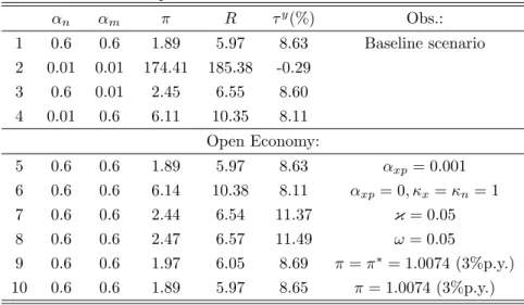
Table 4.1: Optimal inflation and taxes. αn αm π R τk(%) τh(%) τc(%) Obs.: 1 0.6 0.6 0.00 4.00 -15.35 100 -100 Baseline scenario 2 0 0 -3.85 0.00 -15.35 100 -100 3 0.6 0 0.00 4.00 -15.35 100 -100 4 0 0.6 0.00 4.00 -15.35 100 -100 Indexation: 5 0.6 0.6 -3.85 0.00 -15.35 100 -100 κx=κn =κm=κxp= 1 6 0.6 0.6 0.00 4.00 -15.35 100 -100 κx=κn = 1 7 0 0 -3.85 0.00 -15.35 100 -100 κx=κn = 1 8 0.6 0 -3.85 0.00 -15.35 100 -100 κx=κn = 1 9 0 0.6 0.00 4.00 -15.35 100 -100 κx=κn = 1 Open Economy: 10 0.6 0.6 0.00 4.00 -15.35 100 -100 αxp= 0 11 0.6 0.6 -3.85 0.00 -15.35 100 -100 αxp= 0, κx=κn=κm=κxp= 1 12 0.6 0.6 0.00 4.00 -15.35 100 -100 αxp= 0, κx=κn= 1 13 0.6 0.6 0.00 4.00 -13.13 100 -100 κ= 0.01 14 0.6 0.6 0.00 4.00 -13.11 100 -100 ω= 0.01 15 0.6 0.6 0.10 4.10 -15.27 100 -100 π=π∗= 1.0074 (3%p.y.) 16 0.6 0.6 0.00 4.00 -15.35 100 -100 π= 1.0074 (3%p.y.) Profit Taxation: 17 0.6 0.6 0.00 4.00 -15.35 100 -100 τφ= 0 18 0.6 0.6 0.00 4.00 -15.35 100 -100 τφ= 1
that if each country in a single currency area can tax domestic consumption and labor income, the real exchange rate is completely irrelevant to characterize the optimal allocations and welfare.
Table 4.1 describes the optimal choices of nominal interest rates and taxes on capital, labor and consumption under different assumptions regarding nominal rigidities, indexation, parameters charac-terizing the open economy and taxation on profits. Results in the first line are based on the standard calibration described in the previous section. The baseline scenario assumes that taxes on profits are set at the same rate as the tax on capital (τφ=τk) and that there is no price indexation.
There are two striking results in the first panel of table 4.1. First, the degree of nominal rigidity does not affect the optimal policy in terms of nominal interest rates, as there are only two possible outcomes regarding monetary policy: the Friedman rule or price stability. The Friedman rule is the optimal monetary policy under price flexibility or under conditions where the output loss due to sticky prices is removed, like some cases of indexation described below. For every other combination of parameters associated to price rigidities, price stability is the optimal policy outcome. Second, also irrespective of the main parameters of the model, taxation on labor is set at 100%, while the tax on consumption is, actually, a subsidy of 100%. As a matter of fact, the two results are connected. De Fiore and Teles (2003)[16] and Correia, Nicolini and Teles (2008)[14] show that, if the conditions for uniform taxation on consumption goods are satisfied21 and the Friedman rule is the optimal policy, than consumption
must be fully subsidized and labor income fully taxed. One of the reasons for this result is that the number of policy instruments is enough to eliminate distortions generated from frictions affecting the steady state of households and firms allocations in the competitive equilibrium. If this is the case, money becomes nonessential, in the sense that any level of money holdings satisfies the households’ equilibrium conditions, and the Ramsey planner eliminates the cost of shopping by fully subsidizing consumption.
There are three reasons to believe that results described in De Fiore and Teles (2003)[16] and
Correia, Nicolini and Teles (2008)[14] also applies in this framework for small open economies. First, the log-separable utility function in consumption and labor satisfies the implementation conditions for uniform taxation in consumption. Second, the robustness of results in terms of the taxes in consumption and labor even under different parameterization of the model. Third, as presented in lines 17 and 18, is the fact that the Ramsey policy remained exactly the same as in the baseline calibration under different assumptions for taxation on profits. As discussed in SGU (2006)[37], profits are a lump sum transfer from firms to the households. If allowed to set it optimally, the Ramsey planner chooses to confiscate all income from profits to finance its spending with minimum distortion of the households and firms allocations, settingτφ= 1.In the model here, given the large number of policy instruments, the Ramsey planner is indifferent to the inclusion of a lump sum instrument.
The second panel of table 4.1 shows alternative scenarios regarding indexation. Three possible combinations of scenarios can generate the Friedman rule as an outcome for monetary policy. In line 5, with the economy under full indexation, the output loss due to price dispersion across firms is eliminated, generating, in steady state, a similar framework to complete price flexibility. However, as line 6 shows, full indexation is necessary for both production and retail firms, since the policy with indexation present only on production firms is very similar to the baseline scenario in line 1. Lines 7, 8 and 9 show that the Friedman rule might return as a policy outcome with indexation in domestic production firms if prices for imported goods firms are flexible. Thus, the Friedman rule under the current tax system emerges as a solution under a restrict set of conditions: price flexibility; full indexation in prices of domestic firms and retailers; full indexation in prices of domestic firms with price flexibility of imported goods’ retailers. When structural parameters are changed, the tax instrument affected is capital taxation, which is, under the baseline calibration, a subsidy. The intuition for the subsidy in capital was developed in Judd (2002)[23], where the presence of imperfect competition in product markets creates a distortion proportional to the price markup resulting from imperfect competition on the household’s intertemporal substitution of consumption. SGU (2006)[37] explore the properties of the subsidy for the case with depreciation and time-varying capital utilization in a closed economy. Lines 13 and 14 in the table show that parameters related to the open economy framework affect the size of the subsidy, as it declines with a reduction for the demand of imported goods. In order to understand the result, note that the steady state of capital taxes and the return on capital are given by:
τk = 1− rkiµi−a(µi) −1 µz µΥ1−1θ β −1 +δ rik=mciθ ki µz(µΥ)1−1θh i !θ−1
Asκandωapproach zero, the share of total investment based on domestic production increases, as
the total demand of imported goods (cm andim) decreases22. Without the imported good, the demand for domestic goods increases, increasing the marginal return on capital (rk
i) and reducing the subsidy necessary to reduce the distortions from the price markup. Figure 1 shows the subsidy on capital, the capital-labor ratio, the rate of capital utilization and the marginal return of capital net of adjustment costs (rk
iµi−a(µi)) as a function of the share of imported goods in the tradable goods basketκ.
Finally, the only difference in allocations and policies in this setup was found when the inflation in steady state for the foreign economy was larger than zero. However, as the result in line 15 shows, the increase in domestic inflation is smaller than the change in foreign inflation: an inflation of 3% per year in the rest of the world results in an increase of less than 0.1% in inflation under the Ramsey policy.
22Remember, from the optimal choice of households, that
κ is the ratio of imported goods in the basket of tradable
0 0.1 0.2 0.3 0.4 0.5 0.6 0.7 0.8 0.9 −20 −19 −18 −17 −16 −15 −14 −13 Import share τ k 0 0.1 0.2 0.3 0.4 0.5 0.6 0.7 0.8 0.9 31 32 33 34 35 36 37 Import share K/H 0 0.1 0.2 0.3 0.4 0.5 0.6 0.7 0.8 0.9 0.715 0.72 0.725 0.73 0.735 0.74 Import share Capacity Utilization 0 0.1 0.2 0.3 0.4 0.5 0.6 0.7 0.8 0.9 0.036 0.0365 0.037 0.0375 0.038 0.0385 Import share Net Return on K
Figure 1: Optimal taxation on capital and openness
Also notice that this small deviation is a consequence only of foreign inflation, as a positive inflation for domestic prices in the competitive eq