Novel Algorithms For Clustering

(1)

POUR L'OBTENTION DU GRADE DE DOCTEUR ÈS SCIENCES

acceptée sur proposition du jury: Prof. R. West, président du jury Dr F. Fleuret, directeur de thèse Prof. S. Marchand-Maillet, rapporteur

Prof. R. Sznitman, rapporteur Prof. M. Jaggi, rapporteur

Novel Algorithms For Clustering

THÈSE NO 8375 (2018)

ÉCOLE POLYTECHNIQUE FÉDÉRALE DE LAUSANNE PRÉSENTÉE LE 15 FÉVRIER 2018

À LA FACULTÉ DES SCIENCES ET TECHNIQUES DE L'INGÉNIEUR LABORATOIRE DE L'IDIAP

PROGRAMME DOCTORAL EN INFORMATIQUE ET COMMUNICATIONS

Suisse PAR

(2)

(3)

Acknowledgements

This dissertation would not have been possible without the support of several people, to whom I am extremely grateful.

First and foremost, to my PhD supervisor François Fleuret, for his unwavering support. François is an inspiring computer scientist, committed team leader, and kind mentor. To my thesis committee for their constructive feedback, and interest in my research. To the EPFL Doctoral School. Completing my dissertation was smoother than I had anticipated, in large part thanks to their support and planning.

To the administrative team at the Idiap Research Institute, committed to making a productive research environment. My 4+ years in Switzerland have been remarkably hassle free, and I have been able to focus almost entirely on interesting scientific questions. To past and present members of ML Group;Charles Dubout,Leonidas Lefakis,Olivier Canévet,Tatjana Chavdarova,Angelos Katharopoulos,Suraj Srinivas andAlain Rossier.

Our discussions and sharing of research ideas has been stimulating and rewarding. I am glad to have started at the same time as Cijo Jose, who kept us all focused with his frequent ‘What is the most important problem in machine learning?’ question. We may not have a found definitive answer, but I think we have made progress.

While my internship in the Radeon Open Compute team at AMD was not directly related to this thesis, thank you to everyone in Austin who taught me about GPU programming, and expanded my knowledge of the field.

To everyone at Idiap, past and present, for making working and living in Martigny so enjoyable. There are too many people to thank here for all the fun times.

To all the kind people in Lausanne and Martigny who I have been fortunate enough to meet and interact with, at CAS, at the pool, elsewhere. You have all contributed to making this thesis possible.

Finally, to the Hasler Foundation for funding this research through the grant 13018.

(4)

(5)

Abstract

Clustering is a method for discovering structure in data, widely used across many scientific disciplines. The two main clustering problems this dissertation considers are K-means and K-medoids. These are NP-hard problems in the number of samples and clusters, and both have well studied heuristic approximation algorithms. An example is Lloyd’s algorithm for K-means, which is so widely used that it has become synonymous with the problem it attempts to solve.

A large part of this dissertation is about accelerating Lloyd’s algorithm, and its mini-batch andK-medoids variants. The basic tool used to achieve these accelerations is the triangle inequality, which can be applied in a multitude of ways to eliminate costly distance calculations between data samples, as well as to reduce the number of comparisons of these distances.

The first effective use of the triangle inequality to accelerateK-means was by Elkan [2003], with novel refinements appearing more recently in Hamerly [2010]. In Chapter 1 we extend these approaches. First, we show that by using centers stored from previous iterations, one can greatly reduce the number of sample-center distance computations, with substantial improvements in algorithm execution time. We then present an improvement over previous triangle inequality based algorithms for low-dimensions, which uses inter-center distances in a novel way.

Chapter 2 considers the use of the triangle inequality to accelerate the mini-batch variant of Lloyd’s algorithm [Sculley, 2010]. The main difficulty of incorporating triangle inequal-ity bounding in this setting is that clusters can move significantly during the iterations in which a sample is unused, which makes triangle inequality bounding ineffective. We propose a modified sampling scheme to reduce the length of these periods of dormancy, and present an algorithm which achieves an order of magnitude acceleration over the standard mini-batch algorithm.

We then turn attention to theK-medoids problem. In Chapter 3 we focus on the specific problem of determining the medoid of a set. With N samples in Rd, we present a simple algorithm of complexity O(N3/2) to determine the medoid. It is the first sub-quadratic algorithm for this problem whend >1. The algorithm makes use of the triangle inequality to eliminate all but O(N1/2_{) samples as potential medoid candidates.}

Finally, in Chapter 4 we compare differentK-medoids algorithms, and find thatclarans [Ng and Han, 1994], which iteratively replaces randomly selected centers with non-centers, avoids the local minima of other popularK-medoids algorithms. This motivates the use

(6)

of clarans for initializing Lloyd’s algorithm forK-means, which results in improved final energies as compared to K-means++ seeding. We use the triangle inequality to offset the increased computation required by clarans.

Keywords: clustering, triangle inequality, k-means, k-medoids, medoid, mini-batch

(7)

Résumé

Le partitionnement de données est une méthode d’apprentissage non-supervisée qui vise à diviser un ensemble de données en des groupes dans lesquels les données partagent des caractéristiques communes. Les deux problèmes de partitionnement principaux considérés dans cette thèse sont le K-means (K-moyennes) et leK-medoids (K-médoïdes). Ce sont des problèmes NP-difficiles dans le nombre de données et de partitions, pour lesquels il existe des algorithmes heuristiques bien étudiés. Le plus connu de ces algorithmes est celui de Lloyd, que l’on appelle parfois simplement l’algorithme K-means.

Une grande partie de cette thèse porte sur l’accélération de l’algorithme de Lloyd et ses variantes. L’outil de base pour réaliser ces accélérations est l’inégalité triangulaire, qui peut être utilisée de multiples façons pour éliminer des calculs de distance coûteux entre les données, ainsi que pour réduire le nombre de comparaisons de ces distances.

La première utilisation efficace de l’inégalité triangulaire pour accélérer l’algorithme de Lloyd est due à Elkan [2003], avec des améliorations proposées plus récemment par Hamerly [2010] et Ding et al. [2015]. Dans le chapitre 1 nous proposons des améliorations supplémentaires. Tout d’abord, nous montrons qu’en utilisant des centres estimés lors d’itérations précédentes, il est possible de réduire considérablement le nombre de calculs de distances. Ensuite, nous présentons un algorithme qui utilise les distances entre les centres d’une manière nouvelle, qui permet de grandes accélérations en basses dimensions par rapport aux algorithmes existants.

Le chapitre 2 considère l’utilisation de l’inégalité triangulaire pour accélérer la variante mini-batchde l’algorithme de Lloyd. La difficulté principale de l’incorporation de l’inégalité triangulaire ici est que les centres peuvent se déplacer de manière significative au cours des itérations dans lesquelles une donnée est inutilisée, ce qui rend inefficace la technique de délimination. Nous proposons une méthode d’échantillonnage modifiée pour réduire cette période d’inactivité, et nous présentons un algorithme avec une accélération d’un ordre de grandeur par rapport à l’algorithme original du mini-batch.

Nous nous concentrons ensuite sur le problème K-medoids. Dans le chapitre 3, nous abordons le problème spécifique de la détermination du medoid d’un ensemble de N données. Nous présentons un algorithme simple qui est de complexité O(N3/2) dans Rd, le premier algorithme sous-quadratique pour d >1. L’algorithme utilise l’inégalité triangulaire pour éliminer tous les données saufO(N1/2) comme candidats medoids. Enfin, dans le chapitre 4, nous comparons différents algorithmes deK-medoids, et nous montrons que clarans [Ng and Han, 1994], qui échange aléatoirement des centres et

(8)

des non-centres, évite les minima locaux d’autres algorithmes. Cela nous encourage à utiliser claranspour initialiser l’algorithme de Lloyd pour leK-means, ce qui donne des énergies finales améliorées par rapport à K-means++ [Arthur and Vassilvitskii, 2007]. Nous utilisons l’inégalité triangulaire pour réduire la complexité de calcul declarans dans ce contexte.

Mots clés : partitionnement, inégalité triangulaire, k-moyennes, k-médoïdes, médoid, mini-batch

(9)

List of Figures

1.1 Comparing sn- and ns- bounds . . . 13

2.1 Centroid based definitions of redundancy and premature fine-tuning . . . 29

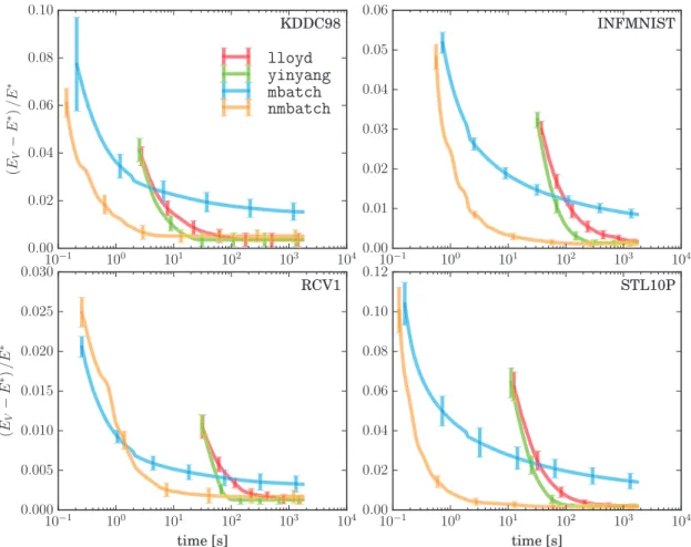
2.2 Mean energy on validation data relative to lowest energy . . . 32

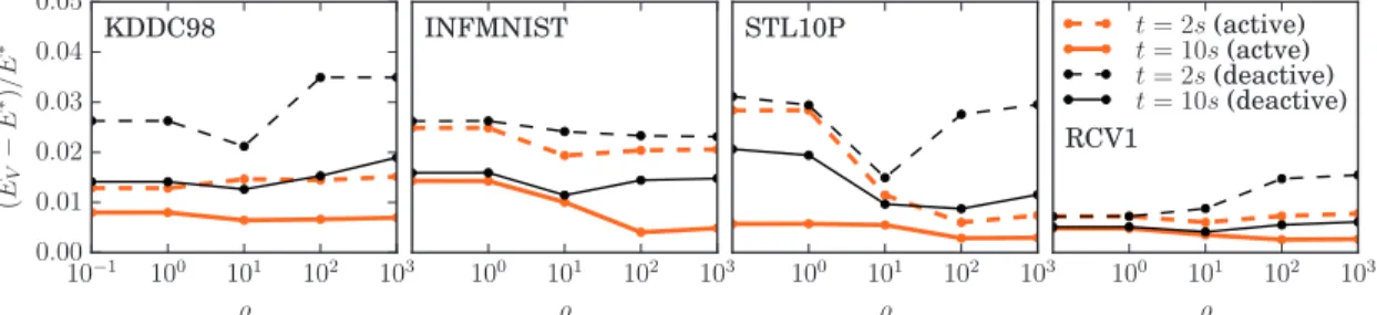
2.3 Relative errors on validation data . . . 33

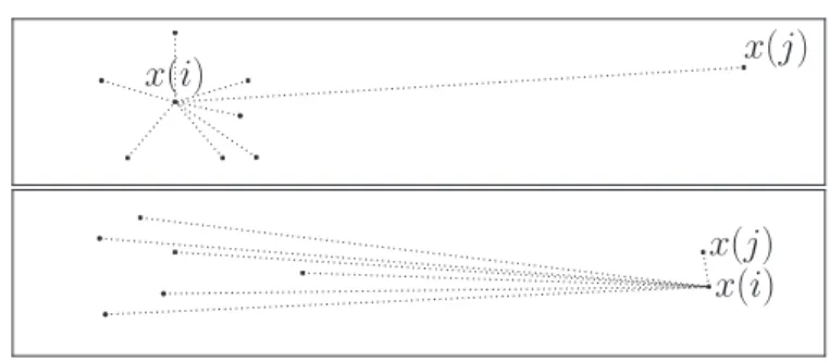
3.1 Using the triangle inequality to eliminate medoid candidates . . . 41

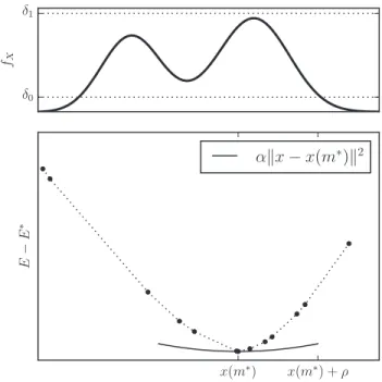
3.2 Illustration of the constants used in Theorem 3.3.2 . . . 43

3.3 Comparison of TOPRANK and trimedon simulated data . . . 45

4.1 Illustrating the importance of good initialization . . . 50

4.2 Illustrating the swap technique . . . 53

4.3 Simulated data in R2 and solutions with differentK-medoids algorithms . 54 4.4 Results on simulated data . . . 54

4.5 The number of consecutive swap proposal rejections . . . 55

4.6 Initialization and final MSEs . . . 58

B.1 Time-energy curves for various ρ . . . 75

B.2 Time-energy curves with bounds disabled . . . 76

B.3 Performace of intermediate algorithms . . . 78

C.1 Number of points computed on simulated data . . . 86

C.2 Summing uniformly distributed cones . . . 87

C.3 Illustrating parametersα,β and ρ . . . 88

C.4 Type 1 elimination . . . 99

D.1 Results on synthetic datasets . . . 103

D.2 Results on real datasets . . . 103

D.3 Illustrating the bounds . . . 110

D.4 Illustrating a bound test . . . 113

D.5 Comparingkm+++clarans+lloyd andkm+++lloyd . . . 119

D.6 Comparing the different optimization levels . . . 120

(14)

(15)

List of Tables

1.1 Datasets used in exact K-Means experiments . . . 16

1.2 Comparison of K-Means implementations . . . 18

1.3 Comparing yinand elk with simplfied versions . . . 19

1.4 Mean runtimes and number of calculations using low-d algorithms . . . . 19

1.5 Counts of times each sn-algorithm is fastest . . . 19

1.6 Measuring the effect of using ns-bounds . . . 20

1.7 Multicore speedups . . . 21

2.1 Comparing implementations of mbatchon INFMNIST and RCV1 . . . 34

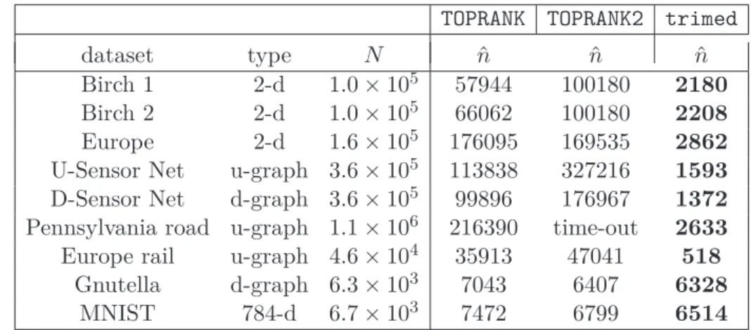
3.1 Comparison of TOPRANK,TOPRANK2and trimedon publicly available data 47 3.2 Relative numbers of distance calculations and final energies . . . 48

4.1 Algorithm complexities at different levels of optimization . . . 56

4.2 Number of distance calculations and time required on simulated data . . . 56

4.3 The datasets used in K-medoids experiments . . . 57

4.4 Summary of results on the 23 datasets . . . 59

A.1 Full names of datasets . . . 69

A.2 Full results withk= 100 . . . 70

A.3 Full results withk= 1000 . . . 71

C.1 Comparison the initialization schemes from Park and Jun [2009] . . . 85

C.2 Table Of Notation For trikmeds . . . 96

D.1 Synthetic datasets used for comparingK-medoids algorithms . . . 102

(16)

(17)

List of Algorithms

1 Cluster assigment, using bounds . . . 25

2 Initialising c,S and v . . . 26

3 Accumulation for sample i . . . 26

4 Mini-batch K-means . . . 26

5 Nested Mini-batch K-means . . . 28

6 The trimedalgorithm for obtaining set medoid . . . 40

7 two-step iterative medlloydalgorithm (vector space, quadratic potential). 52 8 swap-based claransalgorithm (vector space, quadratic potential). . . 52

9 medlloyd algorithm . . . 79 10 RAND algorithm . . . 81 11 TOPRANK algorithm . . . 81 12 TOPRANK2 algorithm . . . 82 13 trikmeds algorithm . . . 92 14 trikmeds initialization . . . 93 15 update-medoids . . . 94 16 assign-to-clusters . . . 95 17 update-sum-bounds . . . 96 18 contiguate . . . 96

19 The pamK-medoids algorithm . . . 104

20 One round of the clarans algorithm . . . 107

21 Unoptimized (level 0) algorithm for computing a proposal energy . . . 107

22 Unoptimized (level 0) algorithm for computing claransassignments . . . 108

23 clarans level 1 optimization . . . 111

24 clarans levels 1 and 2 evaluation of energy of changed cluster . . . 112

25 clarans levels 1 and 2 energy evaluation of all other clusters . . . 112

26 clarans level 1 optimization for updating sample labels and distances . . 114

27 clarans level 2 energy evaluation for non-swapping clusters . . . 115

28 clarans levels 2 energy change evaluation . . . 115

29 clarans level 2 energy update . . . 116

(18)

(19)

Introduction

The goal of machine learning is for computers to learn without being explicitly pro-grammed. The field is commonly divided into two sub-fields, supervised and unsupervised learning. In the supervised setting, the data which the computer learns from consists of pairs, where each pair is an input and desired output. An example of supervised learning is regression, where model parameters are learned to minimize prediction error. The topic of this thesis, clustering, lies in the field of unsupervised learning, where data consists of only inputs; there are no specified ‘correct’ outputs, or labels.

The goal of clustering is to separate data into meaningful groups. It is often used as a first step in exploring new datasets; for example biologists may cluster gene expressions to discover biological pathways, and retailers may cluster customers for targeted marketing. It is also a commonly used technique in signal processing, where values are quantized to satisfy memory/bandwidth constraints.

Clustering techniques can be divided into two categories, hierarchical and flat clustering techniques. An example of hierarchical clustering is the construction of phylogenetic trees, where different tree depths represent different degrees of genetic relatedness; species, genus, family, order, etc. Flat clustering on the other hand assumes no relationship between clusters. This dissertation deals exclusively with the flat variant, commonly referred to aspartitional clustering. This nomenclature can be misleading, as it suggests that hierarchical clustering is non-partitional.

Flat clustering techniques can be further sub-divided into those which aim to minimize a energy function, and those which do not. A popular algorithm where there is no energy function minimization is DBSCAN of Ester et al. [1996], which iteratively agglomerates items into clusters based on estimated point density. Such heuristic algorithms will not be considered in this dissertation, which focuses instead on algorithms which attempt to minimize an energy function.

With the energy minimization approach, an energy function is defined over a parameter-ized set of possible clusterings, and the goal is to minimize this function. The canonical example here is K-means, where the energy function is defined (in a vector space) as the sum over data-points of the squared Euclidean distance to the nearest cluster center.

(20)

List of Algorithms

Another example is spectral clustering of graphs, which attempts to minimize the number of edges between nodes in different clusters. A third example is K-medoids, which generalizesK-means to any loss function but adds the constraint that centers be samples.

Energy minimization clustering problems

Many energy minimization clustering problems such as K-means are NP-hard in the number of samples, and in practice approximation algorithms are used. ForK-means, the most widely used is Lloyd’s algorithm, which relies on a two-step iterative process. In the assignment step, each sample is assigned to the cluster whose center is nearest. In the update step, cluster centers are updated to be the mean of their assigned samples. Lloyd’s algorithm is generally considered to be fast. However, the linear dependence on the number of clusters, the number of samples and the dimension of the space, means that it requires upwards of a billion floating point operations per round on medium-sized datasets. This, coupled with slow convergence and the fact that several runs are often performed to find improved solutions, can make it slow in practice. Accelerating Lloyd’s algorithm will be the focus of Chapter 1 of this dissertation, with special attention paid to the triangle inequality bounding techniques of Elkan [2003].

Lloyd’s algorithm is often referred to as theexact algorithm, which can lead to confusion as it does not solve theK-means problem exactly. The reason for this name is that there are other algorithms which approximate Lloyd’s algorithm. Certain of these rely on a relaxation of the assignment step, for example by only considering certain clusters for each sample, according to some hierarchical ordering [Nister and Stewenius, 2006], or by using an approximate nearest neighbor search, as in Philbin et al. [2007]. Others rely on a relaxation of the update step, for example by using only a subset of data to update centroids [Frahling and Sohler, 2006, Sculley, 2010]. Such relaxations can result in enormous speed-ups for large datasets. These approximate algorithms, in particular the mini-batch K-means algorithm of Sculley [2010] will be the focus of Chapter 2. Lloyd’s algorithm only works in vector spaces, where a ‘mean’ sample, or centroid, can be computed. To generalize the algorithm to any metric space, one can replace centroids with medoids, the cluster elements whose mean energy with other cluster elements is minimal. The resulting K-medoids algorithm can be applied to graph and sequence data. Computing the medoid of a set has applications beyond clustering. In network analysis, the medoid may represent an influential person in a social network, or the most central station in a rail network. In operations research, the facility location problem requires placing one or several facilities so as to minimize the cost of connecting to clients. A simple algorithm for obtaining the medoid of a set ofN elements is to directly compute all inter-element distances, which costs Θ(N2_{). This is in contrast to the computation of} a set mean, which isO(N). In Chapter 3 we consider approximate and exact alternatives for computing the medoid of a set, which reduce this quadratic dependency.

(21)

0.2. Dissertation outline and contributions

Alternatives to Lloyd’s algorithm and itsK-medoids equivalent alluded to in the previous paragraph have been proposed. The majority of these algorithms do not scale linearly in the number of samples. Examples are the algorithm of Kanungo et al. [2002a] and the claransK-medoids algorithm of Ng and Han [1994]. Lloyd’s algorithm islocal, in that far removed centers and points do not directly influence each other. This property contributes to its tendency to terminate in poor minima if not well initialized. Good initialization is key to guaranteeing that the refinement performed by lloyd is done in the vicinity of a good solution, and a topic of active research [Celebi et al., 2013, Bachem et al., 2016]. Theclaransalgorithm is robust to certain local minima of Lloyd’s algorithm, indeed its local minima are a subset of those of Lloyd’s. Initialization and these alternative clustering algorithms will be the topic of Chapter 4, where we consider using clarans for initializing Lloyd’s algorithm.

Dissertation outline and contributions

The four chapters in this dissertation are based on four conference proceedings articles [Newling and Fleuret, 2016a,b, 2017a,b]. While all four chapters are about clustering, they are independent of each other and can be read in any order. Each chapter very closely follows its original paper, with certain connections between the works highlighted where relevant. Notation has been changed from the original papers where appropriate. In Chapter 1, which is based on Newling and Fleuret [2016a], we propose a novel accelerated exactk-means algorithm, which outperforms state-of-the-art low-dimensional algorithm in 18 of 22 experiments, running up to 3×faster. We also propose a general improvement of existing state-of-the-art accelerated exact k-means algorithms through better estimates of the distance bounds used to reduce the number of distance calculations, obtaining speedups in 36 of 44 experiments, of up to 1.8×. We have conducted experiments with our own implementations of existing methods to ensure homogeneous evaluation of performance, and we show that our implementations perform as well or better than existing available implementations. Finally, we propose simplified variants of standard approaches and show that they are faster than their fully-fledged counterparts in 59 of 62 experiments.

In Chapter 2, which is based on Newling and Fleuret [2016b], a new algorithm is proposed which accelerates the mini-batchK-means algorithm of Sculley [2010] by using the distance bounding approach of Elkan [2003]. We argue that, when incorporating distance bounds into a mini-batch algorithm, already used data should preferentially be reused. To this end we propose using nested mini-batches, whereby data in a mini-batch at iteration t is automatically reused at iteration t+ 1. Using nested mini-batches presents two difficulties. The first is that unbalanced use of data can bias estimates, which we resolve by ensuring that each data sample contributes exactly once to centroids. The second is in choosing mini-batch sizes, which we address by balancing premature

(22)

List of Algorithms

fine-tuning of centroids with redundancy induced slow-down. Experiments show that the resulting nmbatch algorithm is very effective, often arriving within 1% of the empirical minimum 100_×earlier than the standard mini-batch algorithm.

In Chapter 3, which is based on Newling and Fleuret [2017a], we present a new algorithm trimedfor obtaining themedoid of a set, that is the element of the set which minimizes the mean distance to all other elements. The algorithm is shown to have, under certain weak assumptions, expected run timeO(N32) inRdwhereN is the set size, making it the

first sub-quadratic exact medoid algorithm for d >1. Experiments show that it performs very well on spatial network data, frequently requiring two orders of magnitude fewer distance calculations than state-of-the-art approximate algorithms. As an application, we show how trimedcan be used as a component in an acceleratedK-medoids algorithm, and then how it can be relaxed to obtain further computational gains with only a minor loss in cluster quality.

In Chapter 4, which is based on Newling and Fleuret [2017b], we show experimentally that the algorithm clarans of Ng and Han [1994] finds better K-medoids solutions than the Voronoi iteration algorithm of Hastie et al. [2001]. This finding, along with the similarity between the Voronoi iteration algorithm and Lloyd’s K-means algorithm, motivates us to useclaransas aK-means initializer. We show thatclaransoutperforms other algorithms on 23/23 datasets with a mean decrease over k-means-++ [Arthur and Vassilvitskii, 2007] of 30% for initialization mean squared error (MSE) and 3% for final MSE. We introduce algorithmic improvements to claranswhich improve its complexity and runtime, making it an extremely viable initialization scheme for large datasets. Finally, in Chapter 5, we summarize our findings and suggest directions for future investigation.

(23)

1

Fast

K

-means with Accurate

Bounds

Chapter introduction

TheK-means problem is to compute a set of K centroids (centers) to minimize the sum over data-points of the squared distance to the nearest centroid. As mentioned in the thesis introduction, it is an NP-hard problem for which the most popular approximation algorithm is Lloyd’s algorithm, often referred to as the K-means algorithm. It has applications in data compression, data classification, density estimation and many other areas, and was recognised in Wu et al. [2008] as one of the top-10 algorithms in data mining.

Recall that Lloyd’s algorithm is also called the exact K-means algorithm, as there is no approximation in the assignment or update step. Note that Lloyd’s algorithm does not state how these steps should be performed, and as such provides a scaffolding on which more elaborate algorithms can be constructed. These more elaborate algorithms, often calledaccelerated exactK-means algorithms, are the primary focus of this chapter. They can be dropped-in wherever Lloyd’s algorithm is used.

Approximate K-means

Alternatives to exactK-means have been proposed. Certain of these rely on a relaxation of the assignment step [Nister and Stewenius, 2006, Philbin et al., 2007]. Others rely on a relaxation of the update step, for example by using only a subset of data to update centroids as in [Sculley, 2010], which will be the focus of Chapter 2.

When comparing approximate K-means clustering algorithms such as those just men-tioned, the two criteria of interest are the quality of the final clustering, and the computational requirements. The two criteria are not independent, making comparison between algorithms more difficult and often preventing their adoption. When comparing accelerated exact K-means algorithms on the other hand, all algorithms produce the

(24)

Chapter 1. Fast K-means with Accurate Bounds

same final clustering, and so comparisons can be made based on speed alone. Once an accelerated exact K-means algorithm has been confirmed to provide a speed-up, it is rapidly adopted, automatically inheriting the trust which the exact algorithm has gained through its simplicity and extensive use over several decades.

Accelerated exact K-means

The first published accelerated K-means algorithms borrowed techniques used to ac-celerate the nearest neighbour search. Examples are the adaptation of the algorithm of Orchard [1991] in Phillips [2002], and the use of kd-trees [Bentley, 1975] in Kanungo et al. [2002b]. These algorithms relied on storing centroids in special data structures, enabling nearest neighbor queries to be processed without computing distances to allK centroids.

The next big acceleration [Elkan, 2003] came about by maintaining bounds on distances between samples and centroids, frequently resulting in more than 90% of distance calculations being avoided. It was later shown [Hamerly, 2010] that in low-dimensions, it is more effective to keep bounds on distances to only the two nearest centroids, and that in general bounding-based algorithms are significantly faster than tree-based ones. Further bounding-based algorithms were proposed by Drake [2013] and Ding et al. [2015], each providing accelerations over their predecessors in certain settings. In this chapter, we continue in the same vain.

Our contribution

Our first contribution (Section 1.3.1) is a new bounding-based accelerated exactK-means algorithm, the Exponion algorithm. Its closest relative is the Annular algorithm [Drake, 2013], a state-of-the-art accelerated exact K-means algorithm in low-dimensions. We show that the Exponion algorithm is significantly faster than the Annular algorithm on a majority of low-dimensional datasets.

Our second contribution (Section 1.3.2) is a technique for making bounds tighter, allowing further redundant distance calculations to be eliminated. The technique, illustrated in Figure 1.1, can be applied to all existing bounding-based K-means algorithms.

Finally, we show how certain of the current state-of-the-art algorithms can be accel-erated through strict simplifications (Section 1.2.2 and Section 1.2.6). Fully paral-lelised implementations of all algorithms are provided under an open-source license at https://github.com/idiap/eakmeans

(25)

1.2. Notation and baselines

Notation and baselines

We describe four accelerated exact K-means algorithms in order of publication date. For two of these we propose simplified versions which offer natural stepping stones in understanding the full versions, as well as being faster (Section 1.4.1).

Our notation is based on that of Hamerly [2010], and only where necessary is new notation introduced. We use for example N for the number of samples and K for the number of clusters. Indices iand j always refer to data and cluster indices respectively, with a sample denoted byx(i) and the index of the cluster to which it is assigned by a(i). A cluster’s centroid is denoted asc(j). We introduce new notation by lettingn1(i) and n2(i) denote the indices of the clusters whose centroids are the nearest and second nearest to samplei respectively.

Note that a(i) andn1(i) are different, with the objective in a round ofK-means being to set a(i) ton1(i). a(i) is a variable maintained by algorithms, changing within loops whenever a better candidate for the nearest centroid is found. On the other hand,n1(i) is introduced purely to aid in proofs, and is external to any algorithmic details. It can be considered to be the hidden variable which algorithms need to reveal.

All of the algorithms which we consider are elaborations of Lloyd’s algorithm, and thus consist of repeating the assignment step and update step, given respectively as

a(i)←n1(i), i∈ {1, . . . , N} (1.1) c(j)←

i:a(i)=jx(i)

i:a(i) =j, j ∈ {1, . . . , K}. (1.2) These two steps are repeated until there is no change to anya(i), or some other stopping criterion is met. We reiterate that all the algorithms discussed provide the same output at each iteration of the two steps, differing only in howa(i) is computed in (1.1).

Standard algorithm (sta)

The Standard algorithm, in this chapter reffered to assta, is the simplest implementation of Lloyd’s algorithm. The only variables kept arex(i) anda(i) fori_{∈ {}1, . . . , N_}andc(j) forj _{∈ {}1, . . . , K_}. The assignment step consists of, for eachi, calculating the distance from x(i) to all centroids, thus revealingn1(i).

Simplified Elkan’s algorithm (selk)

Simplified Elkan’s algorithm, henceforth selk, uses a strict subset of the strategies described in Elkan [2003]. In addition to x(i), a(i) and c(j), the variables kept are

(26)

p(j), the distance moved by c(j) in the last update step, and bounds l(i, j) and u(i), maintained to satisfy,

l(i, j)_≤x(i)₋c(j), u(i)_≥x(i)₋c(a(i)).

These bounds are used to eliminate unnecessary centroid-data distance calculations using,

u(i)< l(i, j) =_⇒x(i)₋c(a(i))<x(i)₋c(j) =_⇒ j=n1(i). (1.3) We refer to (1.3) as aninner test, as it is performed within a loop over centroids for each sample. This as opposed to an outer test which is performed just once per sample, examples of which will be presented later.

To maintain the correctness of the bounds when centroids move, bounds are updated at the beginning of each assignment step with

l(i, j)_←l(i, j)₋p(j), u(i)_←u(i) +p(a(i)). (1.4) The validity of these updates is a simple consequence of the triangle inequality, with a proof in A.1.1. We say that a bound is tight if it is known to be equal to the distance it is bounding, a loose bound is one which is not tight. Forselk, bounds are initialized to be tight, and tightening a bound evidently costs one distance calculation.

When in a given roundu(i)_≥l(i, j), the test (1.3) fails. The first time this happens in a round for sample i, bothu(i) and l(i, j) are loose due to preceding bound updates of the form (1.4). Tightening either bound may result in the test succeeding, but bound u(i) should be tightened beforel(i, j), as it reappears in all tests for sample iand will thus be reused. In the case of a test failure with tight u(i) and loose l(i, j) boundl(i, j) is tightened. A test failure with u(i) and l(i, j) both tight implies that centroid j is nearer to sample ithan the currently assigned cluster centroid, and so a(i) _← j and u(i)←l(i, j).

Elkan’s algorithm (elk)

The fully-fledged algorithm of Elkan [2003], henceforthelk, adds toselkan additional strategy for eliminating distance calculations in the assignment step. Two further variables, cc(j, j′_{), the matrix of inter-centroid distances, and} _s₍_j_{), the distance from} centroid j to its nearest other centroid, are kept. A simple application of the triangle inequality, proved in A.1.2, provides the following test,

cc(a(i), j)

2 > u(i) =⇒ j=n1(i). (1.5)

(27)

1.2. Notation and baselines

Algorithmelk uses (1.5) in unison with (1.3) to obtain an improvement on the test of elk, of the form,

max l(i, j),cc(a(i), j) 2 > u(i) =⇒ j=n1(i). (1.6) In addition to the inner test (1.6), elkuses an outer test, whose validity follows from that of (1.5), given by,

s(a(i))

2 > u(i) =⇒ n1(i) =a(i). (1.7) If the outer test (1.7) is successful, one proceeds immediately to the next sample without changing a(i), thus not only saving K distance calculations but also K floating-point comparisons.

Hamerly’s algorithm (ham)

The algorithm of Hamerly [2010], henceforthham, represents a shift of focus from inner to outer tests, completely foregoing the inner test of elk, and providing an improved outer test.

The K lower bounds per sample of elk are replaced by a single lower bound on all centroids other than the one assigned, defined to satisfy

l(i)≤ min

j=a(i)x(i)−c(j).

The variablesp(j) and u(i) used in elkhave the same definition for ham. The test for a sample iis max l(i),s(a(i)) 2 > u(i) =_⇒ n1(i) =a(i), (1.8) with the proof of correctness being essentially the same as that for the inner test of elk. If test (1.8) fails for sample i, then u(i) is made tight, by computing x(i)₋c(a(i)). If test (1.8) fails with u(i) tight, then all the distances from sample i to centroids are computed, thus revealing n1(i) and n2(i) and allowing the updates a(i) ← n1(i), u(i)_←x(i)₋c(n1(i)) andl(i)← x(i)−c(n2(i)). As with elk, at the start of the assignment step, bounds need to be adjusted to ensure their correctness following the update step. This is done via,

l(i)_←l(i)₋arg max

j=a(i)

(28)

Chapter 1. Fast K-means with Accurate Bounds Annular algorithm (ann)

The Annular algorithm of Drake [2013], henceforth ann, is a strict extension of ham, adding one novel test. In addition to the variables used in ham, one new variableb(i) is required, which roughly speaking is to n2(i) what a(i) is to n1(i). Also, the centroid norms c(j) should be computed and sorted in each round.

Upon failure of test (1.8) with tight bound u(i) in ham, x(i)₋c(j)is computed for all j _{∈ {}1, . . . , K_}to reveal n1(i) andn2(i). With ann, certain of theseK calculations can be eliminated. Define the radius, and corresponding set of cluster indices,

R(i) = max (u(i),x(i)₋c(b(i))),

J(i) ={j:|c(j) − x(i)| ≤R(i)}. (1.9) The following implication, proved in A.1.3, is used

j∈ J(i) =⇒ j∈ {n1(i), n2(i)}.

Thus only distances from sampleito centroids of the clusters whose indices are in_J(i) need to be calculated for n1(i) and n2(i) to be revealed. Oncen1(i) andn2(i) revealed, a(i),u(i) andl(i) are updated as perham, and b(i)_←n2(i).

Note that by keeping an ordering of c(j) the set J(i) can be determined in Θ(log(K)) operations with two binary searches, one for each of the inner and outer radii of _J(i).

Simplified Yinyang (syin) and Yinyang (yin) algorithms

The basic idea with the Yinyang algorithm [Ding et al., 2015] and the Simplified Yinyang algorithm, henceforth yin andsyin respectively, is to maintain consistent lower bounds for groups of clusters as a compromise between the K−1 lower bounds of elkand the single lower bound of ham. In Ding et al. [2015] the number of groups is fixed at one tenth the number of centroids. The groupings are determined and fixed by an initial clustering of the centroids. The algorithm appearing in the literature most similar to yin is Drake’s algorithm of [Drake and Hamerly, 2012], not to be confused with ann. According to Ding et al. [2015], Drake’s algorithm does not perform as well as yin, and we thus choose not to consider it in this chapter.

Denote by Gthe number of groups of clusters. Variables required in addition to those used insta arep(j) andu(i), as per elk,G(f), the set of indices of clusters belonging to the f’th group,g(i), the group to which clustera(i) belongs,q(f) = max_j_∈G₍_f₎p(j), and bound l(i, f), maintained to satisfy,

l(i, f)_≤ arg min

j∈G(f)\{a(i)}

x(i)₋c(j).

(29)

1.3. Contributions and new algorithms

For both syin andyin, both an outer test and group tests are used. To these,yinadds an inner test. The outer test is

min

f∈{1,...,G}l(i, f)> u(i) =⇒ a(i) =n1(i). (1.10) If and when test (1.10) fails, group tests of the form

l(i, f)> u(i) =_⇒ a(i)_{∈ G}(f), (1.11) are performed. As with elk and ham, if test (1.11) fails with u(i) loose, u(i) is made tight and the test reperformed.

The difference between syin and yin arises when (1.11) fails with u(i) tight. With syin, the simple approach of computing distances from x(i) to all centroids in _G(f), then updatingl(i, f), l(i, g(i)), u(i), a(i) andg(i) as necessary, is taken. Withyin a final effort at eliminating distance calculations by the use of a local test is made, as described in A.2.1. As will be shown (Section 1.4.1), it is not clear that the local test of yinmakes it any faster. Finally, we mention howu(i) andl(i, f) are updated at the beginning of the assignment step forsyin and yin,

l(i, f)←l(i, f)−arg max

j∈G(f)

p(a(i)), u(i)_←u(i) +p(a(i)).

Contributions and new algorithms

We first present (Section 1.3.1) an algorithm which we call Exponion, and then (Section 1.3.2) an improved bounding approach.

Exponion algorithm (exp)

Like ann, exp is an extension of hamwhich adds a test to filter out j ∈ {n1(i), n2(i)} when test (1.8) fails. Unlikeann, where the filter is an origin-centered annulus, exphas as filter a ball centred on centroida(i). This change is motivated by the ratio of volumes of an annulus of width r at radiusw and a ball of radius r from the origin, which is dw_rd−1 in Rd. We expectr to be greater thanw, whence the expected improvement. Define,

R(i) = 2u(i) +s(a(i)),

(30)

The underlying test used, proved in A.1.4, is j∈ J(i) =⇒ j∈ {n1(i), n2(i)}.

In moving from anntoexp, the decentralization from the origin to the centroids incurs two costs, one which can be explained algorithmically, the other is related to effective computer memory use.

Recall thatann sortsc(j)in each round, thus guaranteeing that the set of candidate centroids (1.9) can be obtained in O(log(k)) operations. To guarantee that the set of candidate centroids (1.12) can be obtained with O(log(k)) operations requires that c(j)−c(a(i))be sorted. For this to be true for all samples requires sortingc(j)−c(j′) for all j_{∈ {}1, . . . , K_}, increasing the overhead of sorting fromO(klogk) to O(k2_log_k_). The cache memory cost incurred is that, unless samples are ordered bya(i), the bisection search performed to obtain _J(i) is done with a different row of c(j, j′_{) for each sample,} resulting in cache memory misses.

To offset these costs, we replace the exact sorting ofcc with a partial sorting, paying for this approximation with additional distance calculations. We maintain, for each centroid, ⌈log₂k_⌉concentric annuli, each succesive annulus containing twice as many centroids as the one interior to it. For cluster j, annulus f _{∈ {}1, . . . ,_⌈log₂k_⌉} is defined by inner and outer radiie(j, f −1) ande(j, f), and a list of indices w(j, f) with |w(j, f)|= 2f, where

w(j, f) =_{j′:e(j, f ₋1)<c(j′)₋c(j)_≤e(j, f)_}.

Note thatw(j, f) is not an ordered set, but there is an ordering between sets, j′ _∈w(j, f), j′′_∈w(j, f+ 1) =_⇒c(j′)₋c(j)<c(j′′)₋c(j).

Given a search radiusR(i), without a complete ordering ofc(j, j′_{) we cannot obtain}_J₍_i₎ inO(log(k)) operations, but we can obtain a slightly larger set J∗₍_i_{) defined by}

f∗(i) = min_{f :e(a(i), f)_≥R(i)_}, J∗(i) =

f≤f∗₍_i₎

w(j, f),

in log log(k) operations. It is easy to see that_|J∗(i)_{| ≤}2_|J(i)_|, and so using the partial sorting cannot cost more than twice the number of distance calculations.

(31)

1.3. Contributions and new algorithms • • • • • x(i) ct(j) ct+1(j) ct+2(j) ct+3(j)

Figure 1.1 – The classical sn-bound is the sum of the last known distance between the sample to a previous position of the centroid (thick solid line), with all the distances between successive positions of the centroid since then (thin solid lines). The ns-bound we propose uses the actual distance between that previous location of the centroid and its current one (dashed line).

Improving bounds (sn to ns)

In all the algorithms presented so far, upper bounds (lower bounds) are updated in each round with increments (decrements) of norms of displacements. If tests are repeatedly successful, these increments (decrements) accumulate. Consider for example the upper bound update,

ut0+1(i)←ut0(i) +pt0(a(i)),

where subscripts denote rounds. The upper bound afterδtsuch updates without bound tightening is ut0+δt(i) =ut0(i) + t+δt−1 t′₌_t₀ pt′(a(i)). (1.13)

The summation term is a (s)um of (n)orms of displacement, thus we refer to it as an sn-bound and to an algorithm using only such an update scheme as an sn-algorithm. An alternative upper bound at round t0+δtis,

ut0+δt(i) =ut0(i) + t0+δt−1 t′₌_t₀ ct′₊₁(i)−c_t′(i) , =ut0(i) +ct0+δt(i)−ct0(i). (1.14)

Bound (1.14) derives from the (n)orm of a (s)um, and hence we refer to it as an ns-bound. An ns-bound is guaranteed to be tighter than its equivalent sn-bound by a simple application of the triangle inequality, shown in A.1.5. We have presented an upper ns-bound, but lower ns-bound formulations are similar. In fact, for cases where lower bounds apply to several distances simultaneously, due to the additional operation of taking a group maximum, there are three possible ways to compute a lower bound, as

(32)

Chapter 1. Fast K-means with Accurate Bounds

discussed in Appendix A.2.2.

Simplified Elkan’s algorithm-ns (selk-ns)

In transforming an sn-algorithm into an ns-algorithm, additional variables need to be maintained. These include a record of previous centroids C, where C(j, t) =ct(j), and

displacement of c(j) with respect to previous centroids, P(j, t) = c(j)₋ct(j). We

no longer keep rolling bounds for each sample, instead we keep a record of when most recently bounds were made tight and the distances then calculated. For Simplified Elkan’s Algorithm-ns, henceforth selk-ns, we define T(i, j) to be the last time x(i)₋c(j) was calculated, with corresponding distancel(i, j) =x(i)₋c_T₍_i,j₎(j). We emphasize that l(i, j) is defined differently here to inselk, withu(i) similarly redefined asu(i) = x(i)₋c_T₍_i,a₍_i₎₎(a(i)).

The underlying test is

u(i) +P(a(i), T(i, a(i)))< l(i, j)₋P(j, T(i, j)) =_⇒ j=n1(i).

As with selk, the first bound failure for sample iresults in u(i) being updated, with subsequent failures resulting in l(i, j) being updated to the current distance. In addition, whenu(i) (l(i, j)) is updated,T(i, a(i)) (T(i, j)) is set to the current round.

Due to the additional variables C, P and T, the memory requirement imposed is larger withselk-nsthan withselk-sn. Ignoring constants, in roundtthe memory requirement assuming samples of size O(d) is,

memns=O(N d+N k+ktd),

where x, l and C are the principal contributors to the above three respective terms. selk consists of only the first two terms, and so whent > N/min(k, d), the dominant memory consumer in selk-ns is the new variable C. To guarantee that C does not dominate memory consumption, an sn-like reset is performed in rounds {t : t ≡ 0 mod (N/min(k, d))_}, consisting of the following updates,

u(i)←u(i) +P(a(i), T(i, a(i))), l(i, j)_←l(i, j)₋P(j, T(i, j)), T(i, j)_←t,

and finally the clearing ofC.

(33)

1.4. Experiments and results Changing bounds for other algorithms

All sn- to ns- coversions are much the same as that described in Section 1.3.3. We have implemented versions of elk,syinandexpusing ns-bounds, which we refer to aselk-ns, syin-ns and exp-nsrespectively.

Experiments and results

Our first set of experiments are conducted using a single core. We first establish that our implementations of baseline algorithms are as fast or faster than existing implementations. Having done this, we consider the effects of the novel algorithmic contributions presented; simplification, the Exponion algorithm, and ns-bounding. The final set of experiments are conducted on multiple cores, and illustrate how all algorithms presented parallelise gracefully.

We compare 23 K-means implementations, including our own implementations of all algorithms described, original implementations accompanying the papers [Hamerly, 2010, Drake, 2013, Ding et al., 2015], and implementations in two popular machine learning libraries, VLFeat and mlpack. We use the following notation to refer to implementations: {codesource-algorithm}, wherecodesourceis one of bay[Hamerly, 2015],mlp[Curtin et al., 2013],pow [Low et al., 2010],vlf[Vedaldi and Fulkerson, 2008] andown (our own code), and algorithmis one of the algorithms described.

Unless otherwise stated, times are wall times excluding data loading. We impose a time limit of 40 minutes and a memory limit of 4 GB on all {dataset, implementation, K, seed} runs. If a run fails to complete in 40 minutes, the corresponding table entry is ‘t’. Similarly, failure to execute with 4GB of memory results in a table entry ‘m’. We confirm that for all {dataset, K, seed} triplets, all implementations which complete within the time and memory constraint take the same number of iterations to converge to a common local minimum, as expected.

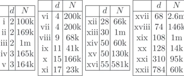
The implementations are compared over the 22 datasets presented in Table 1.1, for K ∈ {100,1000}, with 10 distinct centroid initializations (seeds). For all {dataset,K, seed_} triplets, the 23 implementations are run serially on a machine with an Intel i7 processor and 8MB of cache memory. All experiments are performed using double precision floating point numbers.

Findings in Drake [2013] suggest that the best algorithm to use for a dataset depends primarily on dimension, where in low-dimensions, ham and ann are fastest, in high-dimensions elk is fastest, and in intermediate dimensions an approach maintaining a fractional number of bounds, Drake’s algorithm, is fastest. Our findings corroborate these on real datasets, although the lines separating the three groups are blurry. In presenting our results we prefer to consider a partitioning of the datasets into just two

(34)

Chapter 1. Fast K-means with Accurate Bounds d N i 2 100k ii 2 169k iii 2 1m iv 3 165k v 3 164k d N vi 4 200k vii 4 200k viii 9 68k ix 11 41k x 15 166k xi 17 23k d N xii 28 66k xiii 30 1m xiv 50 60k xv 50 130k xvi 55 581k d N xvii 68 2.6m xviii 74 146k xix 108 1m xx 128 14k xxi 310 95k xxii 784 60k

Table 1.1 – The 22 datasets used in experiments, ranging in dimension from 2 to 784. The datasets come from: the UCI, KDD and KEEL repositories (11,2,2), MNIST and STL-10 image databases (2,1), random (2), European Bioinformatics Institute (1) and Joensuu University (1). Full names and further details in A.3.

groups about the dimension d= 20. ham and its derivatives are considered ford <20, elk and its derivatives ford≥20, andsyin and yinfor all d.

Single core experiments

A complete presentation of wall times and number of iterations for all {dataset, imple-mentation, K} triplets is presented over two pages in Tables A.2 and A.3 (Appendix A.3). Here we attempt to summarise our findings. We first compare implementations of published algorithms (Section 1.4.1), and then show howselkandsyinoften outperform their more complex counterparts (Section 1.4.1). We show thatexp is in general much faster than ann (Section 1.4.1), and finally show how using ns-bounds can accelerate algorithms (Section 1.4.1) .

Comparing implementations of baselines

There are algorithmic techniques which can speedup allK-means algorithms discussed in this chapter, we mention a few which we use. One is pre-computing the squares of norms of all samples just once, and those of centroids once per round. Another, first suggested in Hamerly [2010], is to update the sum of samples by considering only those samples whose assignment changed in the previous round. A third optimization technique is to decompose while-loops which contain inner branchings dependant on the tightness of upper bounds into separate while-loops, eliminating unnecessary comparisons. Finally, while there are no large matrix operations with bounding-based algorithms, in high-dimensions distance calculations can be accelerated by the use of SSE, as in VLFeat, or by fast implementations of BLAS, such as OpenBLAS Xianyi [2016].

Our careful attention to optimization is reflected in Table 1.2 (Section 1.4.1), where implementations of elk, ham, annandyinare compared. The values shown are ratios of mean runtimes using another implementation (column) and our own implementation of 16

(35)

1.4. Experiments and results

the same algorithm, on a given dataset (row). Our implementations are faster in all but 4 comparisons.

Benefits of simplification

We compare published algorithmselk andyinwith their simplified counterparts selk and syin. The values in Table 1.3 are ratios of mean runtimes using simplified and original algorithms, values less than 1 mean that the simplified version is faster. We observe that selk is faster than elk in 16 of 18 experiments, andsyin is faster than yinin 43 of 44 experiments, often dramatically so.

It is interesting to ask why the inventors of elk and yin did not instead settle on algorithmsselkandsyinrespectively. A partial answer might relate to the use of BLAS, as the speedup obtained by simplifyingyin tosyin never exceeds more than 10% when BLAS is deactivated. syin is more responsive to BLAS than yinas it has larger matrix multiplications due to it not having a final filter.

From Annular to Exponion

We compare the Annular algorithm (ann) with the Exponion algorithm (exp). The values in Table 1.4 are ratios of mean runtimes (columnsqt) and of mean number of distance

calculations (columns qau). Values less than 1 denote better performance withexp. We

observe that expis markedly faster thanannon most low-dimensional datasets, reducing by more than 30% the mean runtime in 17 of 22 experiments. The primary reason for the speedup is the reduced number of distance calculations.

Table 1.5 summarises how many times each of the sn-algorithms is fastest on the 44 {dataset, K} experiments, ns-algorithms excluded. The 13 experiments on which exp is fastest are all very low-dimensional (d < 5), the 24 on which syin is fastest are intermediate (8< d <69) and selk orelk are fastest in very high dimensions (d >73). For a detailed comparison across all algorithms, consult Tables A.2 and A.3 (Appendix A.3).

From sn to ns bounding

For each of the 44 {dataset,K} experiments, we compare the fastest sn-algorithm with its ns-variant. The results are presented in Table 1.6. Columns ‘x’ denote the fastest sn-algorithm. Values are ratios of means over runs of some quantity using the ns- and sn- variants. The ratios are qt (runtimes), qa (number of distance calculations in the

assignment step) andqau (total number of distance calculations).

(36)

bay-ham mlp-ham bay-ann pow-yin pow-yin bay-elk mlp-elk vlf-elk

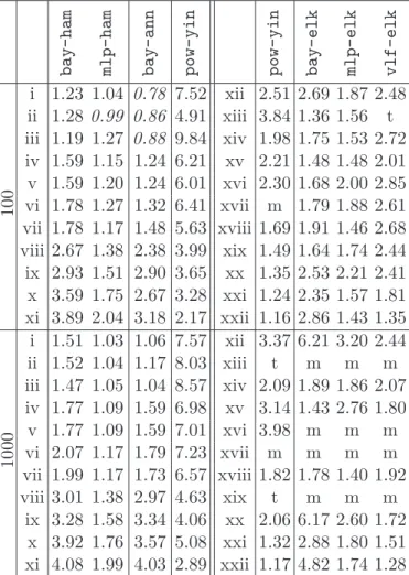
100 i 1.23 1.04 0.78 7.52 xii 2.51 2.69 1.87 2.48 ii 1.28 0.99 0.86 4.91 xiii 3.84 1.36 1.56 t iii 1.19 1.27 0.88 9.84 xiv 1.98 1.75 1.53 2.72 iv 1.59 1.15 1.24 6.21 xv 2.21 1.48 1.48 2.01 v 1.59 1.20 1.24 6.01 xvi 2.30 1.68 2.00 2.85 vi 1.78 1.27 1.32 6.41 xvii m 1.79 1.88 2.61 vii 1.78 1.17 1.48 5.63 xviii 1.69 1.91 1.46 2.68 viii 2.67 1.38 2.38 3.99 xix 1.49 1.64 1.74 2.44 ix 2.93 1.51 2.90 3.65 xx 1.35 2.53 2.21 2.41 x 3.59 1.75 2.67 3.28 xxi 1.24 2.35 1.57 1.81 xi 3.89 2.04 3.18 2.17 xxii 1.16 2.86 1.43 1.35 1000 i 1.51 1.03 1.06 7.57 xii 3.37 6.21 3.20 2.44 ii 1.52 1.04 1.17 8.03 xiii t m m m iii 1.47 1.05 1.04 8.57 xiv 2.09 1.89 1.86 2.07 iv 1.77 1.09 1.59 6.98 xv 3.14 1.43 2.76 1.80 v 1.77 1.09 1.59 7.01 xvi 3.98 m m m vi 2.07 1.17 1.79 7.23 xvii m m m m vii 1.99 1.17 1.73 6.57 xviii 1.82 1.78 1.40 1.92 viii 3.01 1.38 2.97 4.63 xix t m m m ix 3.28 1.58 3.34 4.06 xx 2.06 6.17 2.60 1.72 x 3.92 1.76 3.57 5.08 xxi 1.32 2.88 1.80 1.51 xi 4.08 1.99 4.03 2.89 xxii 1.17 4.82 1.74 1.28

Table 1.2 – Comparing implementations. For 100 (above) and 1000 (below) clusters, and in low- (left) and high- (right) dimensions. Existing implementations (colums) of ham, ann, yin and elk are compared to our implementations as a ratio of mean runtimes, with the mean runtime of our implementation in the denominator. Values greater than 1 mean our implementation runs faster. ‘t’ and ‘m’ are described in paragraph 3 of Section 1.4.

(37)

1.4. Experiments and results own-yin→ own-elk→ own-syin own-selk 100 1000 100 1000 100 1000 i 0.96 0.90 xii 0.58 0.76 xii 0.85 1.05 ii 1.03 0.86 xiii 0.66 0.61 xiii 0.97 m iii 0.88 0.92 xiv 0.50 0.55 xiv 0.84 0.57 iv 0.94 0.87 xv 0.49 0.58 xv 0.54 0.49 v 0.93 0.88 xvi 0.49 0.66 xvi 0.92 m vi 0.91 0.87 xvii 0.44 0.58 xvii 0.75 m vii 0.96 0.90 xviii 0.42 0.47 xviii 0.86 0.66 viii 0.79 0.80 xix 0.36 0.42 xix 0.72 m

ix 0.77 0.80 xx 0.38 0.60 xx 1.12 0.74 x 0.72 0.73 xxi 0.32 0.36 xxi 0.89 0.73 xi 0.64 0.71 xxii 0.36 0.38 xxii 0.99 0.89

Table 1.3 – Comparingyinandelkto simplified versionssyinandselk. Values are ratios of mean runtimes of simplified versions to their originals, for different low-dimensional datasets (rows) and K (columns). Values less than 1 mean that the simplified version is faster. In all but 3 of 62 cases (italicised), simplification results in speedup, by as much as 3_×. own-ann→ own-exp 100 1000 100 1000 qt qau qt qau qt qau qt qau i 0.48 0.52 0.72 0.61 vii 0.71 0.80 0.36 0.32 ii 0.54 0.80 0.58 0.50 viii 1.12 1.24 1.02 0.93 iii 0.53 0.58 0.48 0.44 ix 0.96 0.99 0.73 0.64 iv 0.63 0.80 0.36 0.33 x 0.67 0.65 0.55 0.41 v 0.63 0.80 0.37 0.34 xi 1.24 1.43 1.30 1.16 vi 0.62 0.73 0.42 0.38

Table 1.4 – Ratios of mean runtimes (‘qt’) and mean number of distance calculations

(‘qau’) using the Exponion (own-exp) and Annular (own-ann) algorithms, on datasets

with d < 20. Exponion is faster in all but the four italicised cases. The speedup is primarily due to the reduced number of distance calculations.

ham ann exp syin yin selk elk

0 0 13 24 0 6 1

Table 1.5 – Number of times each sn-algorithm is fastest, over the 44 {dataset, K} experiments, ns-algorithms not considered here.

(38)

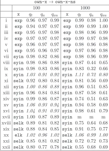
Chapter 1. Fast K-means with Accurate Bounds own-x →own-x-ns 100 1000 x qt qa qau x qt qa qau i exp 0.96 0.97 0.99 exp 0.99 0.98 1.00 ii exp 0.94 0.97 0.97 exp 0.99 0.99 1.00 iii exp 0.95 0.97 0.98 exp 0.98 0.96 0.99 iv exp 0.97 0.97 0.97 exp 0.99 0.97 0.98 v exp 0.96 0.97 0.97 exp 0.98 0.96 0.98 vi exp 0.95 0.96 0.97 exp 0.97 0.96 0.98 vii syin 0.98 0.82 0.86 exp 0.98 0.96 0.99 viii syin 0.98 0.86 0.88 syin 0.87 0.44 0.65 ix syin 0.98 0.83 0.86 syin 0.83 0.32 0.66 x syin 1.03 0.91 0.92 syin 1.11 0.72 0.80 xi selk 0.92 0.80 0.84 syin 0.81 0.56 0.69 xii syin 1.00 0.86 0.88 syin 0.96 0.51 0.85 xiii syin 0.96 0.84 0.84 syin 0.87 0.58 0.61 xiv syin 0.99 0.86 0.87 syin 0.74 0.51 0.63 xv syin 1.06 0.93 0.94 syin 0.94 0.58 0.69 xvi syin 1.04 0.91 0.93 syin 0.98 0.61 0.79 xvii syin 1.00 0.87 0.89 syin m m m xviii selk 0.89 0.81 0.82 syin 0.75 0.64 0.68

xix selk 0.88 0.84 0.85 syin 0.91 0.75 0.77 xx elk 1.02 0.96 1.02 selk 1.06 0.99 1.00 xxi selk 0.85 0.81 0.82 selk 0.72 0.72 0.73 xxii selk 0.80 0.77 0.78 selk 0.55 0.68 0.69

Table 1.6 – The effect of using ns-bounds. Columns ‘x’ denotes the fastest sn-algorithm for a particular {dataset,K} experiment. Columns ‘qt’ denote the ratio of mean runtimes

of ns- and sn- variants of x. Italicised values are cases where using ns-bounding results in a slow down (qt>1), in the majority of cases there is a speedup. ‘qa’ and ‘qau’ denote

ratios of ns- to sn- mean number of distance calculations in the assignment step (a) and in total (au). ‘m’ described in paragraph 3 of §1.4.

up to 45%. As expected, the number of distance calculations in the assignment step is never greater when using ns-bounds, however the total number of distance calculations is occasionally increased due to initial variables being maintained.

Multicore experiments

We have implemented parallelised versions of all algorithms described in this chapter using the C++11 thread support library. To measure the speedup using multiple cores, we compare the runtime using four threads to that using one thread on a non-hyperthreading four core machine. The results are summarised in Table 1.7, where near fourfold speedups are observed.

(39)

1.5. Chapter conclusion and future work i-xi 100 1000 own-exp-ns 0.29 0.31 own-syin-ns0.31 0.29 xii-xxii 100 1000 own-selk-ns0.33 0.30 own-elk-ns 0.30 0.28 own-syin-ns0.27 0.27

Table 1.7 – The median speedup using four cores. The median is over i-xi on the left and xii-xxii on the right.

Chapter conclusion and future work

The experimental results presented show that the ns-bounding scheme makes exact K-means algorithms faster, and that our Exponion algorithm is significantly faster than existing state-of-the-art algorithms in low-dimensions. Both can be seen as good default choices forK-means clustering on large data-sets.

The main practical weakness that remains is the necessary prior selection of which algorithm to use, depending on the dimensionality of the problem at hand. This should be addressed through an adaptive procedure able to select automatically the optimal algorithm through an efficient exploration/exploitation strategy. The second and more prospective direction of work will be to introduce a sharing of information between samples, instead of processing them independently. Finally we mention that for extremely large datasets, only algorithms which are sublinear in the number of datapoints are feasible. This is the topic of the following chapter.

(40)

(41)

2

Nested Mini-Batch

K

-means

Chapter introduction

Given N training samples _X =_{x(1), . . . , x(N)_}in vector space _V, the K-means task is to find C={c(1), . . . , c(K)}in V to minimizeenergy E defined by,