Application of Machine Learning in Well Performance Prediction, Design Optimization and History Matching

(1)

APPLICATION OF MACHINE LEARNING IN WELL PERFORMANCE PREDICTION, DESIGN OPTIMIZATION AND HISTORY MATCHING

A Dissertation by

ADITYA VYAS

Submitted to the Office of Graduate and Professional Studies of Texas A&M University

in partial fulfillment of the requirements for the degree of DOCTOR OF PHILOSOPHY

Chair of Committee, Akhil Datta-Gupta Committee Members, Michael J. King

Bani K. Mallick Duane A. McVay Head of Department, A. Daniel Hill

August 2017

Major Subject: Petroleum Engineering

(2)

ii

ABSTRACT

Finite difference based reservoir simulation is commonly used to predict well rates in these reservoirs. Such detailed simulation requires an accurate knowledge of reservoir geology. Also, these reservoir simulations may be very costly in terms of computational time. Recently, some studies have used the concept of machine learning to predict mean or maximum production rates for new wells by utilizing available well production and completion data in a given field. However, these studies cannot predict well rates as a function of time. This dissertation tries to fill this gap by successfully applying various machine learning algorithms to predict well decline rates as a function of time. This is achieved by utilizing available multiple well data (well production, completion and location data) to build machine learning models for making rate decline predictions for the new wells. It is concluded from this study that well completion and location variables can be successfully correlated to decline curve model parameters and Estimated Ultimate Recovery (EUR) with a reasonable accuracy. Among the various machine learning models studied, the Support Vector Machine (SVM) algorithm in conjunction with the Stretched Exponential Decline Model (SEDM) was concluded to be the best predictor for well rate decline. This machine learning method is very fast compared to reservoir simulation and does not require a detailed reservoir information. Also, this method can be used to fast predict rate declines for more than one well at the same time.

This dissertation also investigates the problem of hydraulic fracture design optimization in unconventional reservoirs. Previous studies have concentrated mainly on

(3)

iii

optimizing hydraulic fractures in a given permeability field which may not be accurately known. Also, these studies do not take into account the trade-off between the revenue generated from a given fracture design and the cost involved in having that design. This dissertation study fills these gaps by utilizing a Genetic Algorithm (GA) based workflow which can find the most suitable fracturing design (fracture locations, half-lengths and widths) for a given unconventional reservoir by maximizing the Net Present Value (NPV). It is concluded that this method can optimize hydraulic fracture placement in the presence of natural fracture/permeability uncertainty. It is also concluded that this method results in a much higher NPV compared to an equally spaced hydraulic fractures with uniform fracture dimensions.

Another problem under investigation in this dissertation is that of field scale history matching in unconventional shale oil reservoirs. Stochastic optimization methods are commonly used in history matching problems requiring a large number of forward simulations due to the presence of a number of uncertain variables with unrefined variable ranges. Previous studies commonly used a single stage history matching. This study presents a method utilizing multiple stages of GA. Most significant variables are separated out from the rest of the variables in the first GA stage. Next, best models with refined variable ranges are utilized with previously eliminated variables to conduct GA for next stage. This method results in faster convergence of the problem.

(4)

iv

DEDICATION

I dedicate this dissertation to my parents, my wife, my brother and my friends for their support during my studies at Texas A&M University.

(5)

v

ACKNOWLEDGEMENTS

I would like to express my sincere gratitude to my advisor, Dr. Akhil Datta-Gupta for his continued guidance during entire period of my PhD study. His expanse of knowledge and readiness to listen to my problems made it possible for me to study in this department of petroleum engineering without any bottlenecks. I would also like to thank him for continued financial support during my entire PhD studies.

I would like to thank Dr. Michael King and Dr. Bani K. Mallick for their continued interest in my research studies. Their immense knowledge and invaluable comments during my presentations guided me to the right direction and also helped me to continue my PhD without any bottlenecks. I would like to thank Dr. Srikanta Mishra from Battelle for his invaluable suggestions regarding Machine Learning study included in this dissertation. His immense knowledge and guidance always helped me when I needed them. I would also like to thank Dr. Duane A. McVay for being a member in my committee.

I would also like to thank Phaedra Hopcus, Barbi Miller and Eleanor Schuler for their help during various occasions particularly with the paperwork involved during this graduate program.

I would also like to thank my colleagues in my research group at the department of Petroleum Engineering, Texas A&M University – Jixiang Huang, Kenta Nakajuma, Hyunmin Kim, Hye Young Jung, Changdong Yang, Atsushi Iino, Tsubasa Onishi,

(6)

vi

Hongquan Chen, Feyisayo Olalotiti-Lawal, Xue Xu, Rongqiang Chen and Gill Hetz - for their invaluable suggestions.

I would also like to alumni of this research group – Xia Xiaoyang, Yanbin Zhang, Peerapong Ekkawong, Jichao Han, Kam Dongjae, Muhammed Al-Rukabi, Jeongmin Kim, Neha Bansal, Shingo Watanabe, Shusei Tanaka and Zheng Zhang - for their invaluable suggestions.

Finally, I would like to thank my professors in University of Oklahoma (where I did my Masters studies) who recommended me to this PhD program – Dr. Deepak Devegowda, Dr. Ramadan Ahmed and Dr. Jeffrey G. Callard.

(7)

vii

CONTRIBUTORS AND FUNDING SOURCES

Contributors

This PhD dissertation work was supervised by Dr. Akhil Datta-Gupta (Committee Chair) and other three committee members - Dr. Michael J. King, Dr. Bani K. Mallick and Dr. Duane A. McVay.

Chapter II of this dissertation study involving Machine Learning based study includes various suggestions made by Dr. Srikanta Mishra from Battelle. This work has been accepted for presentation in one of the SPE conferences before the end of year 2017. Chapter III of this dissertation involving hydraulic fracture optimization study was done in collaboration with Changdong Yang. Changdong Yang provided the upscaling code (Oda Method) and Fast Marching Method (FMM) based forward simulator for this study. This work has been published in Journal of Petroleum Science and Engineering (2017) with a modified workflow.

Chapter IV of this dissertation involving History Matching in Shale Oil reservoirs has been done in collaboration with Atsushi Iino. Atsushi Iino provided the Fast Marching Method (FMM) based reservoir simulator used for this study. This work has been presented in SPE conference (SPE 185719-MS) with a modified workflow and would also be presented in an upcoming URTeC conference (URTeC: 2693139) with a modified workflow.

All remaining work in this dissertation has been done independently by Aditya Vyas.

(8)

viii

Funding Sources

This work was made possible by the financial support of the member companies of Model Calibration and Efficient Reservoir Imaging (MCERI) consortium.

(9)

ix TABLE OF CONTENTS

Page ABSTRACT ...ii DEDICATION ... iv ACKNOWLEDGEMENTS ... v

CONTRIBUTORS AND FUNDING SOURCES ...vii

TABLE OF CONTENTS ... ix

LIST OF FIGURES ... xiii

LIST OF TABLES ... xxxi

CHAPTER I INTRODUCTION AND OBJECTIVES ... 1

1.1 Introduction ... 1

1.2 Dissertation Outline ... 3

CHAPTER II MACHINE LEARNING BASED INSIGHTS ON WELL PERFORMANCE IN EAGLE FORD WELLS ... 5

2.1 Introduction and Literature Review ... 5

2.2 Methodology ... 11

2.2.1 Rate Decline Models ... 11

(10)

x

2.2.1.2 Stretched Exponential Decline Model (SEDM) ... 13

2.2.1.3 Duong Model ... 15

2.2.1.4 Weibull Model ... 15

2.2.2 Machine Learning Algorithms ... 17

2.2.2.1 Random Forests (RF) ... 18

2.2.2.2 Gradient Boosted Machine (GBM) Regression ... 23

2.2.2.3 Support Vector Machines (SVM) Regression or Support Vector Regression (SVR) ... 25

2.2.2.4 Multivariate Adaptive Regression Splines (MARS) ... 26

2.2.3 Model Averaging ... 29

2.2.3.1 Generalized Likelihood Uncertainty Estimation (GLUE)... 31

2.2.4 Relative Influence of Predictor Variables ... 33

2.3 Eagle Ford Field Case Study ... 35

2.4 Summary ... 68

CHAPTER III HYDRAULIC FRACTURE DESIGN AND OPTIMIZATION IN UNCONVENTIONAL SINGLE PHASE GAS RESERVOIR USING GENETIC ALGORITHM ... 69

3.1 Introduction and Literature Review ... 69

(11)

xi

3.2.1 Fast Marching Method ... 78

3.2.2 DFN Upscaling (Oda’s Method) ... 82

3.2.3 Hydraulic Fracturing Design ... 85

3.2.4 Genetic Algorithm and Workflow ... 87

3.3 Results and Discussion ... 91

3.4 Summary ... 107

CHAPTER IV A MULTISTAGE GENETIC ALGORITHM FOR HISTORY MATCHING OF SHALE OIL RESERVOIRS: FIELD CASE STUDY ... 108

4.1 Background and Introduction ... 108

4.2 Methodology ... 109

4.3 Results and Discussion ... 113

4.3.1 History matching results based on GA and three phase FMM... 116

4.3.2 History matching results based on GA and compositional FMM ... 160

4.4Summary... 192

CHAPTER V CONCLUSIONS AND RECOMMENDATIONS ... 193

5.1 Summary and Conclusions ... 193

5.2 Recommendations ... 194

(12)

xii

SUBSCRIPTS ... 198 REFERENCES ... 199 APPENDIX A ... 212

(13)

xiii

LIST OF FIGURES

Page

Figure 2.1 An example well prediction made by Arp’s decline model ... 13

Figure 2.2 Comparison of Arp’s and SEDM decline models ... 14

Figure 2.3 (a) Classification Tree example (b) Equivalent partition for a two variable case ... 20

Figure 2.4 An example Regression Tree from Eagle Ford data predicting maximum oil production ... 20

Figure 2.5 Cost complexity and size of a regression tree against misfit error using Eagle Ford data ... 22

Figure 2.6 Approximate representation of a Gradient Boosted Tree Model ... 24

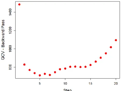
Figure 2.7 An example of GCV plot using Eagle Ford data ... 29

Figure 2.8 Workflow steps for model training and prediction ... 31

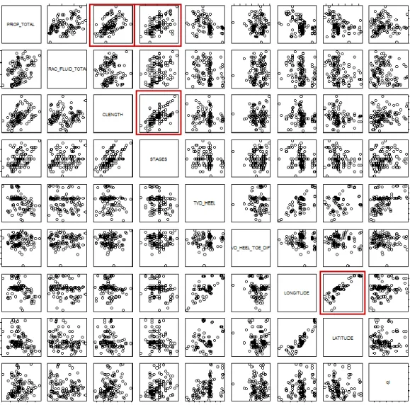
Figure 2.9 Pairwise scatterplots of various predictor variables in Eagle Ford data ... 37

Figure 2.10 Regression Tree fitted on EUR calculated from Arp’s Decline Model ... 38

Figure 2.11 Regression Tree fitted on EUR calculated from SEDM Decline Model ... 38

Figure 2.12 Regression Tree fitted on EUR calculated from Duong’s Decline Model ... 39

(14)

xiv

Figure 2.13 Regression Tree fitted on EUR calculated from Weibull’s Decline Model ... 39 Figure 2.14 Classification Tree fitted on EUR clusters derived from Arp’s Decline

Model ... 40 Figure 2.15 Classification Tree fitted on EUR clusters derived from SEDM Decline

Model ... 40 Figure 2.16 Classification Tree fitted on EUR clusters derived from Duong’s

Decline Model ... 41 Figure 2.17 Classification Tree fitted on EUR clusters derived from Weibull’s

Decline Model ... 41 Figure 2.18 Well clusters based on Initial Flow Rate, qi... 42

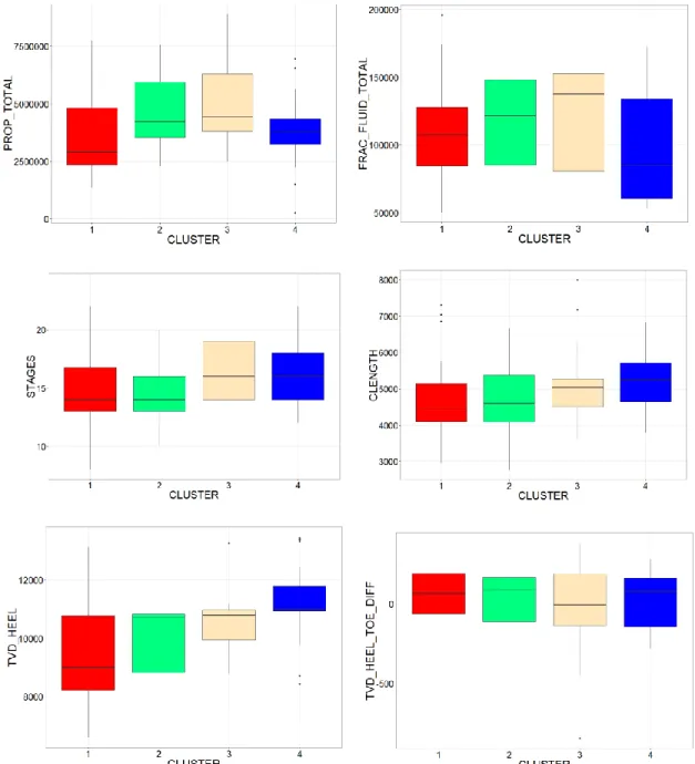
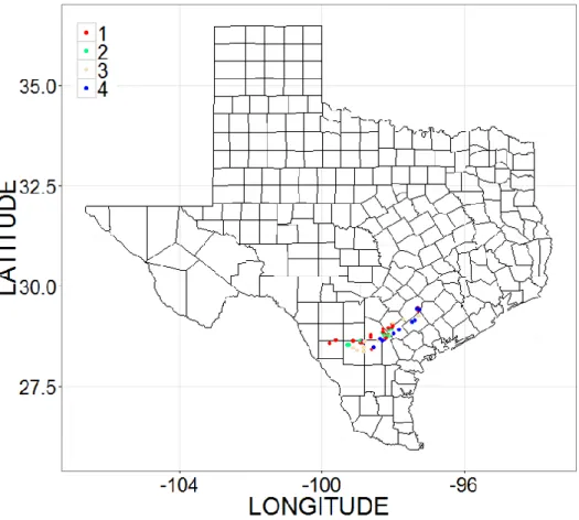
Figure 2.19 Predictor variable distribution in clusters derived from Initial Flow Rate, qi ... 43 Figure 2.20 Study wells on Texas map color coded by cluster number ... 44 Figure 2.21 Correlation between cluster type and different variables ... 45 Figure 2.22 Error metric comparison for different machine learning algorithms

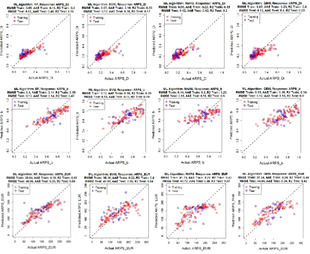
taken into consideration for Arp’s model... 47 Figure 2.23 Scatterplots showing predicted vs actual values of Arp’s decline model

parameters and EUR ... 48 Figure 2.24 Prediction of Arp’s decline curves using GBM ... 49

(15)

xv

Figure 2.25 Error metric comparison for different machine learning algorithms taken into consideration for SEDM model ... 50 Figure 2.26 Scatterplots showing predicted vs actual values of SEDM decline model

parameters and EUR ... 50 Figure 2.27 Prediction of SEDM decline curves using SVM ... 51 Figure 2.28 Error metric comparison for different machine learning algorithms

taken into consideration for Duong’s model ... 52 Figure 2.29 Scatterplots showing predicted vs actual values of Duong’s decline

model parameters and EUR ... 52 Figure 2.30 Prediction of Duong’s decline curves using GBM ... 53 Figure 2.31 Error metric comparison for different machine learning algorithms

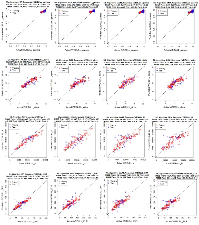
taken into consideration for Weibull model ... 54 Figure 2.32 Scatterplots showing predicted vs actual values of Weibull’s decline

model parameters and EUR ... 55 Figure 2.33 Prediction of Weibull’s decline curves using SVM ... 56 Figure 2.34 Comparison of predictions made by ARP’S - GBM, SEDM - SVM,

DUONG – GBM and WEIBULL - SVM ... 57 Figure 2.35 EUR prediction comparison among best candidates for each decline

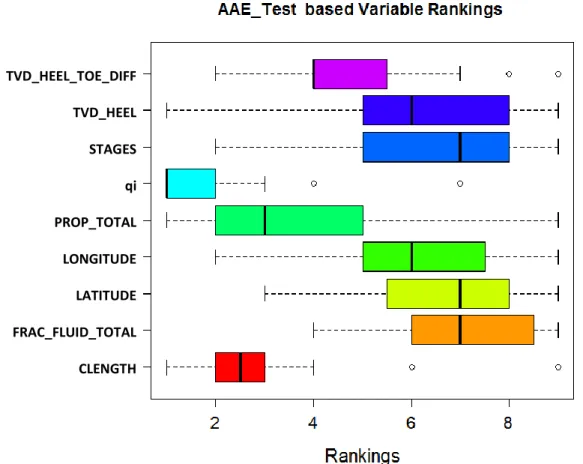
model ... 58 Figure 2.36 RMSE based variable ranking distribution ... 60

(16)

xvi

Figure 2.37 RMSE based variable ranking frequency distribution ... 61

Figure 2.38 RMSE based variable average rank vs rank variance ... 61

Figure 2.39 AAE based Variable Ranking distribution ... 62

Figure 2.40 AAE based variable ranking frequency distribution ... 63

Figure 2.41 AAE based variable average rank vs rank variance... 63

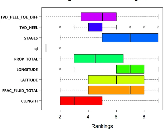
Figure 2.42 R2_{based variable ranking distribution ... 64}

Figure 2.43 R2_{based variable ranking frequency distribution ... 65}

Figure 2.44 R2_{based variable average rank vs rank variance ... 65}

Figure 2.45 Median-Sigma ratio based variable ranking distribution ... 66

Figure 2.46 Median-Sigma ratio based variable ranking frequency distribution ... 67

Figure 2.47 Median-Sigma ratio based variable average rank vs rank variance ... 67

Figure 3.1 Natural Fracture distribution in the base model (Yang et al., 2017)... 83

Figure 3.2 General workflow for genetic algorithm (Yang et al., 2017) ... 89

Figure 3.3 Workflow of objective function evaluation for each model (Yang et al., 2017) ... 91

Figure 3.4 (a) Natural fracture distribution (b) Upscaled reservoir permeability field (Yang et al., 2017) ... 92

Figure 3.5 FMM versus Eclipse simulated gas production for the base model (Yang et al., 2017) ... 93

(17)

xvii

Figure 3.6 Effect of changing minimum matrix permeability during Oda’s

upscaling ... 94 Figure 3.7 a) Gas Rates for various number of fracture stages b) Cumulative Gas

Production for different numbers of fracture stages ... 96 Figure 3.8 Cost and NPV comparison for various cases of number of fracture

stages ... 96 Figure 3.9 Sensitivity analysis of various variables on NPV ... 98 Figure 3.10 NPV distribution in Genetic Algorithm based optimization approach ... 99 Figure 3.11 Distribution of fracture stages and average widths in generation 1 and

generation 25 ... 99 Figure 3.12 Distribution of fracture stages in generation 1 and generation 25 ... 100 Figure 3.13 NPV from Uniform spaced fractures ... 101 Figure 3.14 Hydraulic fracture placement in optimal design using genetic

algorithm ... 102 Figure 3.15 Six possible realizations vs true model/base model in case of

uncertainty in natural fracture distribution ... 104 Figure 3.16 Results of genetic algorithm for multiple realization based

optimization ... 105 Figure 3.17 Variable distribution in the first generation vs last generation ... 105

(18)

xviii

Figure 3.18 Hydraulic fracture placement in optimal design based on multiple

realizations ... 106

Figure 4.1 General workflow for genetic algorithm (GA) ... 113

Figure 4.2 Three regions in the field case reservoir model ... 114

Figure 4.3 Well constraint Tubing Head Pressure during well production period ... 116

Figure 4.4 Cumulative Oil Production of FMM and Eclipse as compared to History data with base case variables (three phase FMM) ... 117

Figure 4.5 Oil Rate Production of FMM and Eclipse as compared to History data with base case variables (three phase FMM) ... 117

Figure 4.6 Cumulative Water Production of FMM and Eclipse as compared to History data with base case variables (three phase FMM) ... 118

Figure 4.7 Water Rate Production of FMM and Eclipse as compared to History data with base case variables (three phase FMM) ... 118

Figure 4.8 Cumulative Gas Production of FMM and Eclipse as compared to History data with base case variables (three phase FMM) ... 119

Figure 4.9 Gas Rate Production of FMM and Eclipse as compared to History data with base case variables (three phase FMM) ... 119

Figure 4.10 Sensitivity analysis at the beginning of Stage 1 (three phase FMM) ... 120

(19)

xix

Figure 4.12 Uncertainty reduction in hydraulic fracture permeability during GA - Stage 1 (three phase FMM) ... 122 Figure 4.13 Uncertainty reduction in hydraulic fracture initial water saturation

during GA - Stage 1 (three phase FMM) ... 122 Figure 4.14 Uncertainty reduction in hydraulic fracture shape factor during GA -

Stage 1 (three phase FMM) ... 123 Figure 4.15 Uncertainty reduction in SRV porosity during GA - Stage 1

(three phase FMM) ... 123 Figure 4.16 Uncertainty reduction in SRV permeability during GA - Stage 1

(three phase FMM) ... 124 Figure 4.17 Uncertainty reduction in SRV initial water saturation during GA -

Stage 1 (three phase FMM) ... 124 Figure 4.18 Uncertainty reduction in SRV shape factor during GA - Stage 1

(three phase FMM) ... 125 Figure 4.19 Variable distribution of hydraulic fracture permeability in the first

generation of GA - Stage 1 (three phase FMM) ... 125 Figure 4.20 Variable distribution of hydraulic fracture initial water saturation in

the first generation of GA - Stage 1 (three phase FMM) ... 126 Figure 4.21 Variable distribution of hydraulic fracture shape factor in the first

(20)

xx

Figure 4.22 Variable distribution of SRV porosity in the first generation of GA - Stage 1 (three phase FMM) ... 127 Figure 4.23 Variable distribution of SRV permeability in the first generation of

GA - Stage 1 (three phase FMM) ... 127 Figure 4.24 Variable distribution of SRV initial water saturation in the first

generation of GA - Stage 1 (three phase FMM) ... 128 Figure 4.25 Variable distribution of SRV shape factor in the first generation of

GA - Stage 1 (three phase FMM) ... 128 Figure 4.26 Variable distribution of hydraulic fracture permeability in the best

selected models of GA - Stage 1 (three phase FMM) ... 129 Figure 4.27 Variable distribution of hydraulic fracture initial water saturation in

the best selected models of GA - Stage 1 (three phase FMM) ... 129 Figure 4.28 Variable distribution of hydraulic fracture shape factor in the best

selected models of GA - Stage 1 (three phase FMM) ... 130 Figure 4.29 Variable distribution of SRV porosity in the best selected models of

GA - Stage 1 (three phase FMM) ... 130 Figure 4.30 Variable distribution of SRV permeability in the best selected models

of GA - Stage 1 (three phase FMM) ... 131 Figure 4.31 Variable distribution of SRV initial water saturation in the best

(21)

xxi

Figure 4.32 Variable distribution of SRV shape factor in the best selected models of GA - Stage 1 (three phase FMM) ... 132 Figure 4.33 Sensitivity analysis at the beginning of Stage 2 (three phase FMM) ... 133 Figure 4.34 GA results for Stage 2 (three phase FMM) ... 134 Figure 4.35 Uncertainty reduction in hydraulic fracture porosity during GA -

Stage 2 (three phase FMM) ... 135 Figure 4.36 Uncertainty reduction in hydraulic fracture permeability during

GA - Stage 2 (three phase FMM) ... 135 Figure 4.37 Uncertainty reduction in hydraulic fracture initial water saturation

during GA - Stage 2 (three phase FMM) ... 136 Figure 4.38 Uncertainty reduction in hydraulic fracture shape factor during

GA - Stage 2 (three phase FMM) ... 136 Figure 4.39 Uncertainty reduction in SRV porosity during GA - Stage 2

(three phase FMM) ... 137 Figure 4.40 Uncertainty reduction in SRV permeability during GA - Stage 2

(22)

xxii

Figure 4.43 Variable distribution of hydraulic fracture porosity in the best selected models of GA - Stage 2 (three phase FMM) ... 139 Figure 4.44 Variable distribution of hydraulic fracture permeability in the best

the best selected models of GA - Stage 2 (three phase FMM) ... 140 Figure 4.46 Variable distribution of hydraulic fracture shape factor in the

best selected models of GA - Stage 2 (three phase FMM) ... 140 Figure 4.47 Variable distribution of SRV porosity in the best selected models of

selected models of GA - Stage 2 (three phase FMM) ... 142 Figure 4.50 Variable distribution of SRV shape factor in the best selected models

of GA - Stage 2 (three phase FMM) ... 142 Figure 4.51 Sensitivity analysis at the beginning of Stage 3 (three phase FMM) ... 143 Figure 4.52 GA results for Stage 3 (three phase FMM) ... 144 Figure 4.53 Uncertainty reduction in hydraulic fracture porosity during GA -

(23)

xxiii

Figure 4.54 Uncertainty reduction in hydraulic fracture permeability during GA - Stage 3 (three phase FMM) ... 145 Figure 4.55 Uncertainty reduction in hydraulic fracture initial water saturation

during GA - Stage 3 (three phase FMM) ... 146 Figure 4.56 Uncertainty reduction in hydraulic fracture shape factor during GA -

Stage 3 (three phase FMM) ... 146 Figure 4.57 Uncertainty reduction in SRV porosity during GA - Stage 3 (three

phase FMM) ... 147 Figure 4.58 Uncertainty reduction in SRV permeability during GA - Stage 3

(three phase FMM) ... 148 Figure 4.61 Variable distribution of hydraulic fracture porosity in the best selected

models of GA - Stage 3 (three phase FMM) ... 149 Figure 4.62 Variable distribution of hydraulic fracture permeability in the best

(24)

xxiv

Figure 4.64 Variable distribution of hydraulic fracture shape factor in the best

selected models of GA - Stage 3 (three phase FMM) ... 150 Figure 4.65 Variable distribution of SRV porosity in the best selected models of

selected models of GA - Stage 3 (three phase FMM) ... 152 Figure 4.68 Combined GA results for all stages (three phase FMM) ... 153 Figure 4.69 Cumulative oil history production data vs simulated production data

(a) in the first stage first generation and (b) including only the best

selected models from the last stage (three phase FMM) ... 154 Figure 4.70 Cumulative water history production data vs simulated production

data (a) in the first stage first generation and (b) including only the best selected models from the last stage (three phase FMM) ... 155 Figure 4.71 Cumulative gas history production data vs simulated production data

(a) in the first stage first generation and (b) including only the best

selected models from the last stage (three phase FMM) ... 156 Figure 4.72 Oil rate history production data vs simulated production data (a) in the

first stage first generation and (b) including only the best selected models from the last stage (three phase FMM) ... 157

(25)

xxv

Figure 4.73 Water rate history production data vs simulated production data (a) in the first stage first generation and (b) including only the best selected models from the last stage (three phase FMM) ... 158 Figure 4.74 Gas rate history production data vs simulated production data (a) in

the first stage first generation and (b) including only the best selected models from the last stage (three phase FMM) ... 159 Figure 4.75 Cumulative Oil Production of FMM vs Eclipse as compared to History

data with base case variables (compositional FMM) ... 161 Figure 4.76 Oil Rate Production of FMM vs Eclipse as compared to History data

with base case variables (compositional FMM)... 161 Figure 4.77 Cumulative Water Production of FMM vs Eclipse as compared to

History data with base case variables (compositional FMM) ... 162 Figure 4.78 Water Rate Production of FMM vs Eclipse as compared to History

data with base case variables (compositional FMM) ... 162 Figure 4.79 Cumulative Gas Production of FMM vs Eclipse as compared to

History data with base case variables (compositional FMM) ... 163 Figure 4.80 Gas Rate Production of FMM vs Eclipse as compared to History data

with base case variables (compositional FMM)... 163 Figure 4.81 Sensitivity analysis at the beginning of Stage 1 (compositional FMM) ... 164 Figure 4.82 GA results for Stage 1 (compositional FMM) ... 165

(26)

xxvi

Figure 4.83 Uncertainty reduction in hydraulic fracture porosity during GA - Stage 1 (compositional FMM) ... 166 Figure 4.84 Uncertainty reduction in hydraulic fracture initial water saturation

during GA - Stage 1 (compositional FMM) ... 166 Figure 4.85 Uncertainty reduction in hydraulic fracture shape factor during GA -

Stage 1 (compositional FMM) ... 167 Figure 4.86 Uncertainty reduction in SRV porosity during GA - Stage 1

(compositional FMM) ... 167 Figure 4.87 Uncertainty reduction in SRV permeability during GA - Stage 1

(compositional FMM) ... 168 Figure 4.88 Uncertainty reduction in SRV shape factor during GA - Stage 1

(compositional FMM) ... 168 Figure 4.89 Variable distribution of hydraulic fracture porosity in the first

generation of GA - Stage 1 (compositional FMM) ... 169 Figure 4.90 Variable distribution of hydraulic fracture initial water saturation in

the first generation of GA - Stage 1 (compositional FMM)... 169 Figure 4.91 Variable distribution of hydraulic fracture shape factor in the first

generation of GA - Stage 1 (compositional FMM) ... 170 Figure 4.92 Variable distribution of SRV porosity in the first generation of GA -

(27)

xxvii

Figure 4.93 Variable distribution of SRV permeability in the first generation of GA - Stage 1 (compositional FMM) ... 171 Figure 4.94 Variable distribution of SRV shape factor in the first generation of

GA - Stage 1 (compositional FMM) ... 171 Figure 4.95 Variable distribution of hydraulic fracture porosity in the best selected

models of GA - Stage 1 (compositional FMM) ... 172 Figure 4.96 Variable distribution of hydraulic fracture initial water saturation in

the best selected models of GA - Stage 1 (compositional FMM) ... 172 Figure 4.97 Variable distribution of hydraulic fracture shape factor in the best

selected models of GA - Stage 1 (compositional FMM) ... 173 Figure 4.98 Variable distribution of SRV porosity in the best selected models of

GA - Stage 1 (compositional FMM) ... 173 Figure 4.99 Variable distribution of SRV permeability in the best selected models

of GA - Stage 1 (compositional FMM) ... 174 Figure 4.100 Variable distribution of SRV shape factor in the best selected models

of GA - Stage 1 (compositional FMM) ... 174 Figure 4.101 Sensitivity analysis at the beginning of Stage 2 (compositional

FMM) ... 175 Figure 4.102 GA results for Stage 2 (compositional FMM) ... 176

(28)

xxviii

Figure 4.103 Uncertainty reduction in hydraulic fracture porosity during GA - Stage 2 (compositional FMM) ... 177 Figure 4.104 Uncertainty reduction in hydraulic fracture permeability during

GA - Stage 2 (compositional FMM) ... 177 Figure 4.105 Uncertainty reduction in hydraulic fracture initial water saturation

during GA - Stage 2 (compositional FMM) ... 178 Figure 4.106 Uncertainty reduction in hydraulic fracture shape factor during GA -

Stage 2 (compositional FMM) ... 178 Figure 4.107 Uncertainty reduction in SRV porosity during GA - Stage 2

(compositional FMM) ... 179 Figure 4.108 Uncertainty reduction in SRV permeability during GA - Stage 2

(compositional FMM) ... 179 Figure 4.109 Uncertainty reduction in SRV initial water saturation during GA -

Stage 2 (compositional FMM) ... 180 Figure 4.110 Uncertainty reduction in SRV shape factor during GA - Stage 2

(compositional FMM) ... 180 Figure 4.111 Variable distribution of hydraulic fracture porosity in the best

selected models of GA - Stage 2 (compositional FMM) ... 181 Figure 4.112 Variable distribution of hydraulic fracture permeability in the best

(29)

xxix

Figure 4.113 Variable distribution of hydraulic fracture initial water saturation in the best selected models of GA - Stage 2 (compositional FMM) ... 182 Figure 4.114 Variable distribution of hydraulic fracture shape factor in the best

selected models of GA - Stage 2 (compositional FMM) ... 182 Figure 4.115 Variable distribution of SRV porosity in the best selected models of

GA - Stage 2 (compositional FMM) ... 183 Figure 4.116 Variable distribution of SRV permeability in the best selected models

of GA - Stage 2 (compositional FMM) ... 183 Figure 4.117 Variable distribution of SRV initial water saturation in the best

selected models of GA - Stage 2 (compositional FMM) ... 184 Figure 4.118 Variable distribution of SRV shape factor in the best selected models

of GA - Stage 2 (compositional FMM) ... 184 Figure 4.119 Combined GA results of all stages (compositional FMM) ... 185 Figure 4.120 Cumulative oil history production data vs simulated production data

(a) in the first stage first generation and (b) including only the best selected models from the last stage (compositional FMM) ... 186 Figure 4.121 Cumulative Water history production data vs simulated production

data (a) in the first stage first generation and (b) including only the best selected models from the last stage (compositional FMM) ... 187

(30)

xxx

Figure 4.122 Cumulative Gas history production data vs simulated production data (a) in the first stage first generation and (b) including only the best

selected models from the last stage (compositional FMM) ... 188 Figure 4.123 Oil rate history production data vs simulated production data (a) in

the first stage first generation and (b) including only the best selected models from the last stage (compositional FMM) ... 189 Figure 4.124 Water rate history production data vs simulated production data (a)

in the first stage first generation and (b) including only the best

selected models from the last stage (compositional FMM) ... 190 Figure 4.125 Gas rate history production data vs simulated production data (a) in

the first stage first generation and (b) including only the best selected models from the last stage (compositional FMM) ... 191 Figure A.1 Input parameters in ML_Algorithms.R script – Part 1 ... 214 Figure A.2 Input parameters in ML_Algorithms.R script – Part 2 ... 215

(31)

xxxi

LIST OF TABLES

Page

Table 2.1: Exponent ‘b’ in Arp’s decline curves ... 12 Table 2.2 Response variables of decline models for Machine Learning... 18 Table 2.3 Most suitable Machine Learning algorithm for each decline model ... 46 Table 3.1 NPV variation with minimum matrix permeability used ... 94 Table 3.2 Economic Parameters for NPV calculations ... 95 Table 3.3 Hydraulic fracture optimization variable ranges ... 97 Table 3.4 NPV values correponding to various realizations vs base model or true

model ... 106 Table 4.1 Uncertainty in Model parameters and their base values for Sensitivity

Analysis (Iino et al., 2017) ... 115 Table A.1 Axis scale values used for Eagle Ford plots ... 217

(32)

1

CHAPTER I

INTRODUCTION AND OBJECTIVES

1.1 Introduction

Reservoir Simulations in large and complex reservoirs can be very costly. Specifically, in unconventional reservoirs, where reservoir models are usually represented by millions of grid cells, oil and gas production forecasts can take a lot of time. Many times, an engineer wants to get a quick idea about how a given well will deplete in future so as to calculate the revenues that will be generated later on. Also, this may be needed even before a detailed geologic information about a new well is provided. Previously, studies have been done to predict maximum/mean oil production in a field using machine learning approaches (LaFollette et. al, 2012 and 2013; Zhong et al., 2015). However, these studies could not predict rate decline with time. The method presented in this chapter can predict decline curve model parameters and predict rate decline for a new well based on data collected from the field. This method is very fast after the needed data has been gathered and properly cleaned/tabulated. In this chapter, this method has been applied to calculate rate decline parameters of four commonly used decline models and also to predict Estimated Ultimate Recovery (EUR) for a new well. This may provide an early estimate of well production for a new well. Also, previous studies involved utilizing a single model based predictions which is not a robust method since it would bias the model towards the training data/machine learning tuning parameters. This chapter takes

(33)

2

advantage of a model averaging technique to make predictions based on weighted average of multiple models built using more than one set of data/tuning parameters.

Another problem under investigation is of finding an optimum hydraulic fracturing design in unconventional reservoirs. Previous studies in the literature involved application of analytical models (e.g., PKN model) to predict well production. However, these models are built for conventional reservoirs and are not suitable to be used in unconventional reservoirs. Also optimization of hydraulic fractures in a given permeability field has been presented earlier (Ma et. al, 2013). However, their study did not take into account the uncertainty in the permeability field. The workflow presented in this chapter can be used to optimize hydraulic fracture design for a given reservoir provided with some uncertainty in the geologic data. This study also discusses uncertainty in the natural fracture distribution and its effects on the Net Present Value (NPV). A synthetic reservoir model has been used for this study and optimization problem is solved for maximizing the NPV. This study also deals with a field-scale case history matching problem in which a base model and parameters with their uncertainty are provided and a genetic algorithm based history matching approach is utilized. Previous studies related to this work involved history matching using a single set of uncertain parameters with a wide range of uncertainty ranges. This chapter study utilizes a multi-stage GA approach that can be used to identify key parameters (heavy-hitters) before proceeding to history matching. First stage of this workflow involves using only the key parameters and matching observed data. In subsequent stages, the refined variables achieved from the first stage are utilized with reduced uncertainty ranges in them. The variables not included in the first stage are

(34)

3

also included in the subsequent stages. This method accelerates the convergence of a stochastic history matching parameter which in this study is Genetic Algorithm (GA). This study also integrates GA with a Fast Marching Method (FMM) based reservoir simulator which is a faster alternative to commonly used commercial simulators. In this study, simulated cumulative oil, water and gas production have been matched with their corresponding observed/history data provided by the field operator. A production forecast has also been made and corresponding production has been compared to test the accuracy of history matching algorithm.

1.2 Dissertation Outline

This dissertation document contains several chapters each containing a different case study. In Chapter II, Eagle Ford well data has been gathered from a publicly available website and used with several machine learning algorithms in order to build models that can predict rate declines for a new well. This method is very fast after the needed data has been gathered and properly cleaned/tabulated. It can be used to calculate rate decline parameters of commonly used decline models and also to predict Estimated Ultimate Recovery (EUR) for a new well. This may provide an early estimate of well production for a new well.

In Chapter III, a detailed workflow for hydraulic fracture design optimization has been presented. This workflow based on genetic algorithm can be used to optimize hydraulic fracture design for a given reservoir provided the geologic data including permeability and porosity is known. This study also briefly discusses about the uncertainty

(35)

4

in the natural fracture distribution and its effects on the optimization of Net Present Value (NPV). A synthetic reservoir model has been used for this study and optimization problem is solved for maximizing the NPV.

In Chapter IV, a field case study has been presented in which a set of uncertain parameters/variables with production history data are provided and objective is to match history data by applying genetic algorithm based workflow. A multi-stage GA approach has been used in this study to accelerate the convergence of GA. The multi-stage GA approach utilizes heavy hitter variables in the first stage to fine tune the variables making most impact. Subsequent stages, however include all variables with updated uncertainty ranges. Simulated cumulative oil, water and gas production have been matched with their corresponding observed/history data provided by the field operator. A production forecast has also been made and corresponding actual production has been compared to test the accuracy of history matching algorithm.

Finally, in Chapter V, conclusions from this dissertation study have been presented and recommendations for possible extension/improvement to current work are suggested.

(36)

5

CHAPTER II

MACHINE LEARNING BASED INSIGHTS ON WELL PERFORMANCE IN EAGLE FORD WELLS

2.1 Introduction and Literature Review

Oil and gas wells have been in existence for a long time but it was only in recent times when importance of large sets of well data are realized by the petroleum industry. A large set of well data which includes well location data and well completion data are becoming available in a format that can be easily used by data scientists. Since shale oil and gas revolution started in USA, a large number of wells have been drilled and their data collected. Many of these data are available in publically accessible websites on internet. This chapter deals with a study done using well data collected from more than 100 wells in the Eagle Ford reservoir. Well data used for this study include well location/depth parameters including latitude, longitude and total vertical depth and well completion parameters including number of hydraulic fractures, volume of fracturing fluid used, amount of proppant used, and completed length. Well data has been collected from the online database DrillingInfo. Only oil wells have been selected for this study.

Lee et al. (2002) applied classification and non-parametric regression algorithms for electrofacies characterization and permeability prediction in complex reservoirs. Model based clustering technique was used to identify clusters from well log responses. For each cluster, non-parametric regression technique was utilized to build model and predict corresponding permeability. The non-parametric regression algorithms include

(37)

6

ACE (Alternating Conditional Expectation), GAM (Generalized Additive Model) and NNET (Neural Networks). ACE based regression algorithm outperformed the other two regression methods in this study.

Perez et al. (2005) applied classification trees with well log response to predict electrofacies, lithofacies and hydraulic flow units in uncored wells. This study also reported the predictor variables that have most influence in classification tree based prediction. It was also reported that larger trees may be too sensitive to the statistical noise present in the data and therefore smaller (pruned) trees should be used for such kind of study.

Mishra (2012) reported a method to make predictions based on multiple models instead of single one. The final prediction is based on weighted average of predictions from all models. It was shown that more than one decline model can be fitted to a data with acceptable accuracy. However, their future predictions may vary a lot. To overcome this problem, the final predicted response variable, Estimated Ultimate Recovery (EUR) was predicted using multiple models aggregated together by Generalized Likelihood Uncertainty Estimation or GLUE (Beven and Binley, 1992; Neuman, 2003; Singh et al. 2010) methodology.

LaFollette and Holcomb (2011) presented data analytic results using Barnett shale horizontal wells. It was found that wells more than 3,500 – 4,500 ft of lateral length were less efficient in terms of production per foot. Also, it was found that, most wells are drilled in approximately 140 and 320 degrees of azimuth. Also, the best wells were those that were drilled near horizontal.

(38)

7

LaFollette et al. (2012) reported results for Bakken formation of the Eastern Williston Basin. They found production efficiency (production per foot of completed lateral) decreases with increasing lateral length. It shows that increasing number of stages and completed length alone did not find positive correlation with maximum monthly oil production (calculated during first 12 month production period). However, proppant concentration seemed to have a positive correlation with maximum monthly oil production.

LaFollette et al. (2012) presented results of North Texas Barnett Shale wells with emphasis on well completion and fracture stimulation. It was concluded in this paper that traditional linear regression methods are not suitable for this kind of data: prone erroneous data, missing data, non-linear data and data containing subtle interrelationships among variables. It was concluded that boosted tree method is more suited for this kind of data for regression purposes. The study also found a good correlation between maximum monthly oil production and amount of fracturing fluid used for fracking in the wells studied.

LaFollette (2013) presented data analytics results from Barnett shale and Bakken Shale. In Barnett shale case, relative influence of various variables in predicting maximum monthly gas production during first 12 month period was studied. TVD is found to be the most influential factor in this study using boosted tree model. In Bakken shale case, relative influence of various variables in predicting maximum monthly oil production during first 12 month period was studied. In this case, well location coordinates were found to be most influential in the study done using boosted tree model.

(39)

8

LaFollette et al. (2013) reported results using well data gathered from Bakken Light Tight Oil Play. This study was carried out using multivariate analysis of production data. It was found that well location that can be used as a proxy for reservoir quality is one of the most influential predictor for production forecast. It was also concluded that longer lateral wells are less efficient in terms of production per feet of lateral length.

LaFollette et al. (2014) reported results using well data gathered from Eagle Ford Formation in South Texas. This study carried out multivariate analysis on Eagle Ford production data. Reservoir quality was proxied by X-Y surface location since petrophysical data was unavailable. The completion variables used for this study included proppant amount, volume of fracturing fluid used, number of fracturing stages, and completed length (measured as difference between measured depths of bottom perforation and top perforation). Other variables included dip, azimuth and GOR. The proxies for production efficiency include maximum oil rate, barrels of oil produced per unit completed length and barrels of oil produced per pound of proppant used. The paper also reported trends in reservoir fluid parameters.

The study reported that GOR and well location are among the most important variables influencing multivariate analysis. This study also reported that even though production rates increases with increase in completed lateral length, the production per unit completed length reduces as completed length increases. Increase in proppant amount used for completion jobs is found to increase productivity in terms of maximum monthly production.

(40)

9

Holcomb et al. (2015) studied the productivity effects from spatial placement and well architecture in Eagle Ford shale horizontal wells. This study found that wells drilled and completed in GOR less than 5000 scf/bbl have lower maximum monthly oil production (during first 12 month period) per foot of length but then appear to have a lower percentage decline rate than higher GOR wells. This study could not find direct correlation between increased proppant consumption and increased well productivity.

Zhong et al. (2015) reported their results with Wolfcamp shale. They applied several machine learning algorithms to build models that can predict first 12 months of cumulative oil for oil wells. Machine learning algorithms used included Ordinary Least Squares (OLS), Support Vector Machines (SVM), Random Forests (RF) and Gradient Boosting Model (GBM). In their results, RF modeled the data most accurately. Also, they reported the predictor relative importance based on R2_{loss. In this method, each of the}

predictor variable was removed from predictor set one at a time while keeping rest of the predictors intact and checking the change in R2, i.e., R2 loss. The predictor having more R2 loss associated with it is considered more important. Different machine learning algorithms had different ranking/predictor importance order in this study. In case of RF, fracturing fluid amount used for completion job turned out to be most influential factor.

Schuetter et al. (2015) reported their machine learning study using data set comprising wells in Wolfcamp Shale in West Texas (Delaware Basin and Central Basin). Response variable in this study was cumulative production in the first 12 months of oil production period. This study tried to predict first 12 month cumulative production for new test data wells based on machine learning models developed using training wells.

(41)

10

Machine learning algorithms used here were Ordinary Least Squares, Random Forest, Gradient Boosting Machine, Support Vector Regression (SVR) and Kriging. K-fold cross-validation technique was utilized to avoid overfitting. It was found that although Kriging based models fits training data perfectly, they did not perform well for test data. Also, study includes relative importance study of various predictor variables. It was found that TVD is most influential predictor among all predictors.

Centurion et al. (2012) presented their data analytics results using Eagle Ford well data. It was pointed out that most of the top productive wells in Eagle Ford lie in the counties of Dewitt and Karnes. However, the worst performing wells are not located in a particular location. Also, the wells completed using delayed release production chemicals have higher productivity than those which didn’t use those chemicals. In the multivariable statistical analysis, most dominant predictors were identified and they included proppant volume, injection rates, treatment pressure, measured depth of deepest perforation, production chemicals combined with stimulation fluids and porosity indicator.

Centurion et al. (2013) reported their multivariate analysis results using Eagle Ford well data. The most significant variables found in their study were proppant per ft, pressure, cluster spacing, thickness, average porosity and perforation length.

Centurion et al. (2014) reported their data analytic results using LaSalle County wells in Eagle Ford shale. Cumulative oil production during first 3 months was considered as a proxy for well productivity. Multivariate analysis results showed most influential variables in this region to be completed length and stage spacing. Proppant pumped showed positive correlation with well productivity. Also, increased shut-in time between

(42)

11

hydraulic fracture treatment and the first day of production also had a positive effect on well productivity. Reduction in well spacing led to lower initial productivity but increased overall productivity of the region in a longer term.

2.2 Methodology

Eagle Ford well data has been downloaded from drillinginfo (website: info.drillinginfo.com). More than 100 well data has been collected and analyzed using various machine learning techniques. First, well data has been analyzed using exploratory data analytic techniques such as scatterplot and boxplot. Next, machine learning techniques such as Random Forest (RF), Gradient Boosted Machine (GBM), Support Vector Machine (SVM) and Multivariate Adaptive Regression Splines (MARS) have been utilized in order to predict rate decline in Eagle Ford wells. Since the production rate data of these wells are mostly noisy, it is difficult to model them with smooth models. However, a novel approach explained in this section can handle this problem using machine learning algorithms in conjunction with decline rate models used in oil industry. The well rate data is first fitted with one of the commonly used decline models listed below.

2.2.1 Rate Decline Models 2.2.1.1 Arp’s Decline Model

Arp’s decline equation (Arps, 1945) can be represented as follows:

q(t) = 𝑞𝑖 (1+𝑏𝐷𝑖𝑡) 1 𝑏 (2.1) where,

(43)

12

𝑞(𝑡) = rate at time t (STB/D)

𝑞_𝑖 = initial rate (STB/D)

𝐷_𝑖 = initial decline rate (1/month)

𝑏 = hyperbolic decline coefficient (dimensionless)

𝑡 = time (months)

Exponent b in above equation shows type of decline in a well (Table 2.1).

Table 2.1: Exponent ‘b’ in Arp’s decline curves

b value Decline type

b = 0 Exponential

0 < b < 1 Hyperbolic

b = 1 Harmonic

Fig. 2.1 shows an example well’s predictions made by Arp’s decline model keeping Initial flow rate, Di same but varying exponent, b. It may be seen that for higher

(44)

13

Figure 2.1 An example well prediction made by Arp’s decline model

2.2.1.2 Stretched Exponential Decline Model (SEDM)

Valko and Lee (2010) presented Stretched Exponential Decline Model which is a specialized decline model for unconventional reservoirs and predicts rate decline in transient flow regime. Since unconventional wells produce in transient flow regimes, SEDM is more suitable for them compared to Arp’s decline model. Eq. 2.2 shows SEDM equation.

q(t) = 𝑞_𝑖𝑒𝑥𝑝 [− (_𝜏𝑡)𝑛] (2.2)

where,

𝑞(𝑡) = rate at time t (STB/D)

𝑞_𝑖 = initial rate (STB/D)

𝜏 = characteristic relaxation time (month)

(45)

14

Johnston (2006) explained stretched exponential decay process as a sum of exponential decay with a “fat tailed” probability distribution of time constants. Valko and Lee (2010) explained SEDM to be a sum of large number of individual exponential decays. It was also reported by Valko and Lee (2010) that Arp’s may predict physically unrealistic Estimated Ultimate Recovery (EUR) values for b ≥ 1 but SEDM will always give finite value of EUR. Fig. 2.2 shows how Arp’s can fit early rate data really well but would over predict production at long term period.

(46)

15

2.2.1.3 Duong Model

Duong (2011) presented following equation in the case of fracture dominated flow characteristics. This equation (Eq. 2.3) is derived empirically for shale gas and tight gas reservoirs.

q(t) = 𝑞1𝑡−𝑚𝑒𝑥𝑝 (_1−𝑚𝑎 (𝑡1−𝑚− 1)) (2.3)

where,

𝑞(𝑡) = rate at a time t (STB/D)

𝑞₁ = flow rate on first day (STB/D)

𝑎 = intercept constant

𝑚 = slope parameter. Duong (2011) showed that for the unconventional reservoirs m > 1

2.2.1.4 Weibull Model

Another way to model decline curve is through Weibull growth curve (Weibull, 1951; Mishra, 2012).This equation (Eq. 2.4) is generally used for modeling time-to-failure in applied engineering problems.

𝑃(𝑡) ≡ 𝐺_𝑃 = 𝑀 {1 − 𝑒𝑥𝑝 (− (_𝛼𝑡)𝛾)} (2.4)

where,

𝐺_𝑃 = cumulative production at time t

𝑀 = carrying capacity (Max. cumulative production)

(47)

16

𝛼 = scale parameter

Differentiating Eq. 2.4 gives (Weibull, 1951; Mishra, 2012):

q(t) = 𝑀_𝛼𝛾(_𝛼𝑡)𝛾−1𝑒𝑥𝑝 (− (_𝛼𝑡)𝛾) (2.5) where,

𝑞(𝑡) = rate at time t (STB/month)

M, the carrying capacity, is the maximum cumulative production set by this equation. This means that cumulative production cannot reach unrealistic values as in the Arp’s model in some cases. Since it is a fitting parameter like 𝛼 and 𝛾, a close approximate value of M is needed to fit Weibull curve on a well rate decline data. For this study, cumulative well oil production during the available well oil production period with ± 10 % margin has been assumed for best range within which M should lie. 𝛼 , the scale parameter, is that value of time at which (1-1/e) or 63.2% of the resources have been produced (Mishra, 2012). 𝛾, the shape factor, shows how rate of growth changes with time and is usually less than 1 for unconventional reservoirs (Mishra, 2012).

Once the well rate data is collected for all the wells included in this study, all of the above decline models are used to fit them with a best match and the parameters of corresponding decline models are stored for further study. Also, the Estimated Ultimate Recovery (EUR) for each well is calculated as a numeric integral of monthly oil production over 30 year period (360 months):

𝐸𝑈𝑅 = ∑360𝑖=1𝑞𝑖 (2.6)

(48)

17

𝐸𝑈𝑅 = Estimated Ultimate Recovery

𝑞_𝑖 = monthly oil rate (STB/month) of 𝑖𝑡ℎ month

2.2.2 Machine Learning Algorithms

Once well rate data is collected and fitted with the decline models discussed previously, the data is tabulated such that each row corresponds to a well and each column corresponds to one of the variables (predictors or responses). Table 2.2 shows the response and predictor variables used for each of the decline curve models. As shown in

Table 2.2, predictor variable are unchanged across each of the decline models but response variables change.

The data table is divided randomly into 80% - 20% partition so that 80% of the rows are utilized to train machine learning model (called as training data) and remaining 20% of the rows are used for testing (called as test data) the model accuracy. In this study, different machine learning algorithms have been applied to the data under investigation. Following subsections briefly presents the main idea behind some of these algorithms that provided better results than the remaining ones. The three machine learning algorithms that produced better prediction results than others are: Random Forests (RF), Gradient Boosted Machines (GBM) and Support Vector Machines (SVM). However, results for Multivariate Adaptive Regression Splines (MARS) are also shown in this chapter for comparison purposes only.

(49)

18

Table 2.2 Response variables of decline models for Machine Learning

Arp’s SEDM Duong Weibull

Response

Variables 𝐷_𝑖, 𝑏, 𝐸𝑈𝑅 𝑡𝑎𝑢, 𝑛, 𝐸𝑈𝑅 𝑎, 𝑚, 𝐸𝑈𝑅 𝛾, 𝛼, 𝑀, 𝐸𝑈𝑅

Predictor Variables

Well Latitude and Longitude, TVD, Difference between TVDs of Heel and Toe, Completed Length, Number of Fracture stages, Amount of fracturing

fluid and Proppant used for fracking

Once a model has been trained, it can then predict the decline curve parameters of new wells which in this case are test data wells. Oil rate decline with respect to time can then be predicted by using decline curve parameters and corresponding decline equation.

This study also deals with finding the relative influence of various predictor variables for building a model. This can be regarded as a variable importance or sensitivity study in which it is possible to identify most important and least important predictor variables to build a model.

A short description of four of the machine learning algorithms applied to Eagle Ford study is presented in the following sections.

2.2.2.1 Random Forests (RF)

Breiman (2001) reported an ensemble based learning method based on Classification and Regression Trees (CART) concept. A single Classification Tree consists of a series of partition such that each partition divides data points into two

(50)

19

dissimilar groups as shown in Fig. 2.3 (a). However, in reality, a partition by linear boundaries may not be able to partition data into pure classes. This is shown in Fig. 2.3 (b) by impurities of whites among black colored circles and impurities of blacks among white circles. These impurities can be minimized by further partitioning the variable space. The mathematical quantity to be minimized here is called the Gini Impurity Index (Breiman, 1996) which is a measure of impurities present in a given partition/compartment.

𝐺𝑖𝑛𝑖 𝐼𝑚𝑝𝑢𝑟𝑖𝑡𝑦 𝐼𝑛𝑑𝑒𝑥 = ∑𝑘 𝑝_𝑖(1 − 𝑝_𝑖)

𝑖=1 = 1 − ∑𝑘𝑖=1𝑝𝑖2 (2.7)

where,

𝑝_𝑖 = probability of training dataset belonging to 𝑖𝑡ℎ class

𝑘 = number of classes (or categorical variables)

In a pure node (consisting only of one type of class), this Gini Index should be equal to 0. In order to partition a variable space, different possibilities are tested including different variables and different point of partition in a given variable’s range. This is repeated at each node until Gini’s Index is minimized or number of terminal nodes exceed the specified set limit. The final prediction value at a terminal node is governed by majority vote.

(51)

20

(a) (b)

Figure 2.3 (a) Classification Tree example (b) Equivalent partition for a two variable case

Regression Trees are similar to a Classification Trees but in their case prediction is made for a continuous variable (real number) instead of a categorical variable (class) as shown in Fig. 2.4.

Figure 2.4 An example Regression Tree from Eagle Ford data predicting maximum oil production

(52)

21

The values at each node is calculated by minimizing Residual Sum of Squares (RSS) using Eqs. 2.8 and 2.9 (Shalizi, 2006):

𝑅𝑆𝑆 = ∑𝑛𝑐=1∑𝑛𝑖=1𝑐 (𝑦𝑖 − 𝑚𝑐)2 (2.8) 𝑚_𝑐 =_𝑛1 𝑐∑ 𝑦𝑖 𝑛𝑐 𝑖=1 (2.9) where, 𝑐 = number of nodes

𝑛𝑐 = number of data points in a node 𝑦_𝑖 = observed or actual response value

In order to partition a variable space, different possibilities are tested including different variables and different point of partition in a given variable’s range. This is repeated at each node until RSS is minimized or number of terminal nodes exceed the specified set limit. The final prediction value at a terminal node is governed by mean prediction value. Cost Complexity (Cp) in a regression tree (Perez et. al, 2003) is given by:

Cp = Training Error + k × No. of terminal nodes (2.10) where,

k = cost complexity factor. If k = 0, tree will not control no. of terminal nodes and only error rates are involved making tree larger than needed. If k is very large, tree will be very short with high training error and biased model

Fig. 2.5 shows Cp vs cross validation error/misfit error in Eagle Ford data. As can

be seen in this figure tree size of 2 gives minimum Cp. However, it must be noted that a very small size of tree can bias the model for the training data. In the Random Forest

(53)

22

package in R, tree sizes are controlled by providing a range within which total number of terminal nodes should lie. This is an indirect way of controlling Cp. The default minimum number of nodes is 5 for regression trees in Random Forest package used in this study. Therefore in the example shown below, the tree size of 5 would be appropriate.

Figure 2.5 Cost complexity and size of a regression tree against misfit error using Eagle Ford data

(54)

23

A Random Forest (Breiman, 2001) is an ensemble based machine learning algorithm which is comprised of a large number of uncorrelated trees (Classification or Regression Trees). Instead of fitting data with a single Classification or Regression Tree, a random forest of multiple uncorrelated trees is constructed. Each tree is derived from a bootstrap subsample of given data as well as a bootstrap subsample of variables from predictor variable set leading to a different order of partitioning. During prediction process for a new dataset (not used for training the Random Forest), final prediction is based on majority vote (Random Forest of Classification Trees) or averaged response (Random Forest of Regression Trees).

2.2.2.2 Gradient Boosted Machine (GBM) Regression

Gradient Boosted Machine (Friedman, 2001 and 2002) is an ensemble tree based machine learning algorithm in which a true model is represented by a series of trees such that each subsequent tree is fitting the error residual of the previous tree (Fig. 2.6). Friedman (2001 and 2002) reported that “Gradient Boosting of the regression trees produces competitive, highly robust, interpretable procedures for both regression and classification, especially mining less than clean data”.

(55)

24

Figure 2.6 Approximate representation of a Gradient Boosted Tree Model (Modified from Gradient Boosted Regression Trees in scikit-learn,

https://www.slideshare.net/DataRobot/gradient-boosted-regression-trees-in-scikitlearn)

A simple mathematical formulation of gradient boosted trees is presented below (source: scikit-learn.org website (http://scikit-learn.org/stable/modules/ensemble.html). A general form of additive model is given by:

𝐹(𝑥) = ∑𝑀𝑚=1𝛾𝑚ℎ𝑚(𝑥) (2.11)

𝛾_𝑚 = step length

ℎ_𝑚(𝑥) = basis functions

The gradient boosting additive model can be represented as:

𝐹𝑚(𝑥) = 𝐹𝑚−1(𝑥) + 𝛾𝑚ℎ𝑚(𝑥) (2.12)

where,

ℎ_𝑚(𝑥) = regression/classification tree used as a basis functions/weak learners

For each stage, ℎ𝑚(𝑥) is chosen to minimize the loss function L for the given model 𝐹𝑚−1

and its fit 𝐹𝑚−1(𝑥𝑖)

𝐹_𝑚(𝑥) = 𝐹𝑚−1(𝑥) + 𝑎𝑟𝑔 min_ℎ ∑𝑛𝑖=1𝐿(𝑦𝑖, 𝐹𝑚−1(𝑥𝑖) − ℎ(𝑥)) (2.13)

(56)

25 𝐹𝑚(𝑥) = 𝐹𝑚−1(𝑥) + 𝛾𝑚∑𝑛𝑖=1∇𝐹𝐿(𝑦𝑖, 𝐹𝑚−1(𝑥𝑖)) (2.14) where, 𝛾_𝑚 = 𝑎𝑟𝑔 min 𝛾 ∑ 𝐿 (𝑦𝑖, 𝐹𝑚−1(𝑥𝑖) − 𝛾 𝜕𝐿(𝑦𝑖,𝐹𝑚−1(𝑥𝑖)) 𝜕𝐹𝑚−1(𝑥𝑖) ) 𝑛 𝑖=1 (2.15)

The initial model, 𝐹₀(𝑥) is usually chosen to be the mean of target values in case of regression problems.

2.2.2.3 Support Vector Machines (SVM) Regression or Support Vector Regression (SVR)

Smola and Schölkopf (2004) presented Support Vector Regression (SVR) or Support Vector Machine (SVM) Regression which has become quite successful among machine learning algorithms. This algorithm tries to fit function, f(x), on a given training dataset such that the maximum deviation of a data point from this function is equal to ε. However, complexity of f(x) is controlled so that f(x) is kept as flat as possible.

Eq. 2.16 shows the term that is needed to be minimized and Eq. 2.17 shows that constraints used while minimizing Eq. 2.16.

Objective is to find: 𝑓(𝑥⃗) = 𝑤⃗⃗⃗. 𝑥⃗ + 𝑏, by:

minimizing: 1₂‖𝑤‖2+ 𝐶 ∑𝑁𝑖=1(𝜉𝑖+ 𝜉𝑖∗) (2.16)

subjected to constraints: {

𝑦_𝑖− (𝑤⃗⃗⃗. 𝑥⃗ + 𝑏) ≤ 𝜀 + 𝜉_𝑖 𝑦𝑖 − (𝑤⃗⃗⃗. 𝑥⃗ + 𝑏) ≤ −(𝜀 + 𝜉𝑖∗)

𝜉_𝑖, 𝜉_𝑖∗_{> 0} (2.17)

Eq. 2.16 also shows the slack term variables (Cortes and Vapnik, 1995, Smola and Schölkopf, 2004) in order to avoid overfitting in the model. The second term in Eq. 2.16

(57)

26

shows the cost term containing slack variables, 𝜉𝑖, 𝜉𝑖∗ which include points with deviations

more than 𝜀 . By controlling the constant C (where C > 0), the contribution of the second term in Eq. 2.16 can be controlled. This is also a way to control the trade-off between the flatness of f(x) and the limit up to which data points having deviations larger than ε are tolerated in the machine learning model. Using Lagrange multipliers (𝛼_𝑖, 𝛼_𝑖∗) to solve above minimization problem, the above equations become:

𝑤 = ∑𝑙𝑖=1(𝛼𝑖 − 𝛼𝑖∗)𝑥𝑖 (2.18)

𝑓(𝑥) = ∑𝑙𝑖=1(𝛼𝑖− 𝛼𝑖∗) < 𝑥𝑖, 𝑥 > + 𝑏 (2.19)

where,

𝛼𝑖, 𝛼𝑖∗= Lagrange multiplier <. , . > = dot product

Aizerman et al. (1964) and Nilsson (1965) showed how to map a training data to some feature space ℱ i.e., Φ: Χ → ℱ. This process simplifies the problem such that the optimization problem tries to find function f(x) in the feature space and not in actual input space.

𝑓(𝑥) = ∑ (𝛼_𝑖− 𝛼_𝑖∗_)𝑘(𝑥

𝑖, 𝑥) + 𝑏 𝑙

𝑖=1 (2.20)

Once the data is in feature space, the function f(x) to be fitted can be more flat than fitting it in original data space.

2.2.2.4 Multivariate Adaptive Regression Splines (MARS)

Freidman (1991 and 1993) reported Multivariate Adaptive Regression Splines (MARS). Eq. 2.21 shows the basic form of MARS: