Paroxysmal atrial fibrillation prediction based on HRV analysis and non-dominated sorting genetic algorithm III

(1)

Contents lists available at ScienceDirect

Computer

Methods

and

Programs

in

Biomedicine

journal homepage: www.elsevier.com/locate/cmpb

Paroxysmal

atrial

ﬁbrillation

prediction

based

on

HRV

analysis

and

non-dominated

sorting

genetic

algorithm

III

K.H. Boon

∗

, M. Khalil-Hani

, MB Malarvili

FacultyofElectricalEngineering,UniversitiTekonologiMalaysia,Skudai,Johor81310,Malaysia

a

r

t

i

c

l

e

i

n

f

o

Articlehistory: Received 17 February 2017 Revised 27 August 2017 Accepted 10 October 2017 Keywords:

Heart rate variability Paroxysmal atrial ﬁbrillation Arrhythmia prediction Multi-objective optimization

Non-dominated Sorting genetic algorithm III Feature selection

a

b

s

t

r

a

c

t

This paper presents a method that able to predict the paroxysmal atrial fibrillation (PAF). The method uses shorter heart rate variability (HRV) signals when compared to existing methods, and achieves good prediction accuracy. PAF is a common cardiac arrhythmia that increases the health risk of a patient, and the development of an accurate predictor of the onset of PAF is clinical important because it increases the possibility to electrically stabilize and prevent the onset of atrial arrhythmias with different pacing techniques. We propose a multi-objective optimization algorithm based on the non-dominated sorting genetic algorithm III for optimizing the baseline PAF prediction system, that consists of the stages of pre-processing, HRV feature extraction, and support vector machine (SVM) model. The pre-processing stage comprises of heart rate correction, interpolation, and signal detrending. After that, time-domain, frequency-domain, non-linear HRV features are extracted from the pre-processed data in feature extraction stage. Then, these features are used as input to the SVM for predicting the PAF event. The proposed optimization algorithm is used to optimize the parameters and settings of various HRV feature extraction algorithms, select the best feature subsets, and tune the SVM parameters simultaneously for maximum prediction performance. The proposed method achieves an accuracy rate of 87.7%, which significantly outperforms most of the previous works. This accuracy rate is achieved even with the HRV signal length being reduced from the typical 30 min to just 5 min (a reduction of 83%). Furthermore, another significant result is the sensitivity rate, which is considered more important that other performance metrics in this paper, can be improved with the trade-off of lower specificity.

1. Introduction

Atrial Fibrillation (AF) is the common non-life-threatening car-

diac arrhythmia that can lead to stroke, heart failure, and other

heart related disease [1,2]. Patients often start with episodes of

paroxysmal atrial ﬁbrillation (PAF), which last from seconds to

days but it is self-terminating. It also can be treated by medica- tion or electrical shock issued by the Implantable Deﬁbrillator De-

vice (ICD) [3]. However, the PAF can slowly evolve to the chronic

AF that cannot return to normal sinus rhythm even with external treatment. Therefore, the development of an accurate predictor of

the onset of PAF is clinically important because it increases the

possibility to electrically stabilize and prevent the onset of atrial

arrhythmias with different pacing techniques [4]. This can lead to

decrease in symptoms, and possibly a decrease in atrial remodel- ing that causes increased susceptibility to future episodes of PAF

[3].

∗ _{Corresponding author.}

E-mail addresses: [email protected] (K.H. Boon), [email protected] (M. Khalil-Hani), [email protected] (M. Malarvili).

Much research have been done for developing a method that

can predict the onset of PAF based on electrocardiogram (ECG)

signal. The works can be divided into premature atrial complexes

(PAC) detection [5–7] and heart rate variability (HRV) analysis [8–

13]. Tables 5 and 6 summarizes their methodology and prediction performance. Almost all existing methods, which achieved acceptable prediction accuracies (around 80% and above), employed

30 min signal for feature extraction [8]. Some of them [5,9,10] even

could achieve same or above the level of 90%.

Previous works also attempted to use the HRV signal shorter

than 15 min for prediction. However, their accuracy rates were

lower when compared to the methods that used 30 min signal.

For example, Boon et al. [8] proposed a HRV analysis prediction

method based on HRV analysis, and they achieved accuracy rate of 79.3% and 68.9% for 15 min and 10 min respectively. Yang and Yin

[12] achieved lowest accuracy rate with 57% when they extracted features from 10 min HRV signal based on footprint analysis. With

spectral features, Hickey and Heneghan [6] achieved prediction ac-

curacies of 68%, 70%, and 66% for 5, 10 and 30 min of HRV signal respectively.

(2)

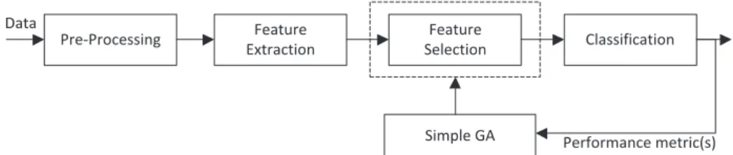
Fig.1. Block diagram of typical feature selection based on simple GA.

Therefore, this main objective of this paper is to propose a PAF onset prediction method that requires shorter time duration of the HRV signal during the feature extraction, while improving the prediction accuracy level.

2. Optimizationmethod

Multiple features are usually extracted during the HRV analysis. However, using all features does not always give the best classiﬁ-

cation performance due to the curse of dimensionality [14]. There-

fore, feature selection algorithm is usually used to improve the per-

formance. The feature selection is an optimization problem that

involves selecting the best combination of features from the original extracted features without transforming them. It can enhance the performance, reduce the number of features, and help the re- searchers to understand which features are important to the clas- siﬁcation model.

Genetic algorithm (GA) is one of the popular methods for fea-

ture selection. Fig.1 shows the block diagram of the typical fea-

ture selection model based on simple GA for the existing research

based on HRV analysis [8,15–19]. After the features are extracted

from the pre-processed data, the simple GA is used to select the feature subset with high classiﬁcation performance. Based on crit- ical review, there are a few shortcomings for the feature selection

model in Fig.1.

One of the shortcomings is the parameter values and settings in

both HRV pre-processing and feature extraction stages are not opti-

mized (tuned) for maximum classiﬁcation performance. As shown

in Fig. 1, before the feature selector is applied, the HRV features

must be extracted based on certain pre-deﬁned values and ﬁxed setting of HRV feature extraction algorithms. According to Rashedi

et al. [20], to maximize the performance of extracted features,

these parameters should be tuned simultaneously with the feature selection process for different application and database. They proposed a heuristic search method called gravitational search algo-

rithm (GSA) to optimize the image recognition system. It simul-

taneously optimized both the parameters of feature extraction algorithms (wavelet transform and color histogram) and the feature subset, and this improved detection rate of their system. Inspired by their work, this paper intends to propose an optimization algorithm that can simultaneously optimizes the parameters in pre- processing and feature extraction stages, feature subset in feature selection process, and parameters of classiﬁcation model. Such op-

timization model is shown in Fig.2.

Another shortcoming is that the trade-off between the classification sensitivity and specificity rate is not considered. Improving certain amount of sensitivity may need to sacrifice certain degree

of speciﬁcity, or vice versa [21]. Some medical applications require

high sensitivity while other need high speciﬁcity [21]. For example,

Xie and Minn [22] and Koley and Dey [23] developed the algorithm

for detecting the sleep apnea based on ECG signal. They were interested in high sensitivity rate because it reduced the risk of over- looking the apnea events that could pose threats to the patients. In this paper, we are more interested in improving the sensitivity at the expense of acceptable reduction in speciﬁcity rate when pre-

Heart Rate Correction

Interpolation

SVM

HRV Feature Extraction Supervised Prediction

Detrending Time Domain Analysis Frequency Domain Analysis Non-linear Analysis Detrended HRV

HRV Features Predicted Event HRV Data

HRV Pre-processing

Corrected HRV

Proposed optimization algorithm based on NSGA-III

Baseline prediction system based on HRV

Optimizing

Fig.2. Overview of the proposed method.

dicting the PAF onset. Therefore, the trade-off between different

prediction performance metrics is considered when developing the optimization algorithm.

In this paper, optimizing the PAF onset prediction model is

a multiple-objective problem. When GA is used for this class of

problems, there are two common approaches: weighted sum, and

Pareto dominance concept [24]. The former case is used in sim-

ple GA, in which multiple objective ﬁtness functions are linearly

combined with different weight coeﬃcients into a single composite

function. It was employed in previous works [8,18,19] to combine

different performance metrics (i.e., sensitivity, speciﬁcity, accuracy rate and feature count). There are several drawbacks with this ap-

proach [24]. One of them is that the trial and error is required for

tuning the weights values in order to obtain a solution with de- sired performance. Moreover, the simple GA only can return single solution per optimization run. As a result, the GA needs to be run multiple times for obtaining multiple solutions before trade- off among the solutions can be analyzed, which is not convenience for designer. It should be noted that, although the ﬁtness functions

in previous works [8,18,19] had multiple metrics, they did not per-

form the trade-off analysis because their interest was obtaining a single solution with highest accuracy. The drawbacks in the simple GA can be tackled by using the Pareto dominance concept based GA. In this paper, the state-of-the-art Pareto dominance based GA,

which is called non-dominated sorting genetic algorithm III (NSGA-

III) [25,26], is adopted for optimization.

Finally, the GA based feature selectors in HRV based previous

works [8,15–19] are belong to the type of wrapper method [27] be-

cause only the machine learning classiﬁer is used to evaluate the

ﬁtness of the chromosome. Wrapper method has a well-known

shortcoming: the risk of selecting a subset that is overﬁtting to

the trained supervised classiﬁer [8,27]. In the non-HRV research,

the hybrid feature selection based on simple GA [28–30] has been

proposed to mitigate this issue to certain degree. The hybrid GA uses the ﬁlter method (i.e., statistical test or correlation measure) to evaluate the feature, and only selects the feature that can pass certain evaluation criterion during the formation of feature subset.

(3)

the filter method called Mann-Whitney U test with the simple GA based feature selector. Before the GA was applied, they filtered out the HRV features that could not pass the U test at 20% significance

level. Therefore, in this paper, the ﬁlter method is used as part

of the proposed optimization algorithm for evaluating the features before they are selected to form feature subset.

In this paper, a multi-objective optimization algorithm based on NSGA-III is proposed to optimize the PAF onset prediction system while considering the above-mentioned shortcomings. The layout

of the paper is as follows. Section3 presents the database and pro-

posed method. Results and discussion are presented in Section4.

Finally, conclusion and future works are given in the Section5.

3. Proposedmethod

Fig. 2 shows overview of the proposed prediction method. It

comprises of the stages of pre-processing, HRV feature extraction, and support vector machine (SVM) model, which are simultaneously optimized by the proposed optimization algorithm based on NSGA-III. Initially, 5 min HRV data that immediately precedes the PAF event is fed to the pre-processing stage for heart rate correc-

tion, interpolation and signal detrending. They are two types of

pre-processed output: corrected HRV and detrended HRV. It should

be noted that the detrended HRV is also corrected and interpo-

lated. Then, 6 time-domain and 4 non-linear features are extracted based on the corrected HRV, while 43 frequency-domain features are extracted based on the detrended HRV. Finally, these features are used as input to the SVM model for predicting the PAF event.

The SVM is implemented by using the C ++ library called LIBSVM

[31].

3.1. Experimentaldata

Based on the previous works [6–13], 106 data from 53 pairs of

ECG recordings (each pair is recorded from different PAF patients) are obtained from the standard database called Atrial Fibrillation

Prediction Database (AFPDB) [32]. Each pair of data contains one

30 min ECG segment that ends just prior to the onset of PAF event and another 30 min ECG segment at least 45 min distant from any onset of PAF. Each ECG segment contains two-channel traces from Holter recording with sampling rate of 128 Hz and 12-bit resolu- tion.

In this paper, the 5 min HRV segment that at least 45 min dis-

tant from the PAF event is assigned a class label of “NORMAL”,

while the HRV segment that immediately precedes the PAF event is given a class label of “ABNORMAL”.

3.2. Preprocessing

In the preprocessing stage, the RR intervals (intervals between successive R peaks) are derived from the ECG signal by using the

Hamilton and Tompkins algorithm [33]. Then, the HRV data is com-

puted as the reciprocal of RR intervals. After that, the HRV data

segment sequentially goes through the heart rate correction, in-

terpolation and signal detrending. The heart rate correction and

signal detrending are performed based on the McNames algorithm

[34] and the high pass ﬁlter proposed by Tarvainen et al. [35] respectively. As for the interpolation process, either linear or cubic

spline method is used to resample the HRV data to certain fre-

quency (4 Hz or 7 Hz) [36]. The methodology and reason for op-

timizing these 3 pre-processing steps with the proposed algorithm

are discussed in Section3.5.2.

3.3. HRVfeatureextraction

Fifty-three well-established HRV features are extracted using

time-domain, frequency domain and non-linear analysis [37]. Their

abbreviations are listed in TableA.1 and explained in the follow-

ing sub-sections. It should be noted that, they are one or more input parameters for the feature extraction algorithms that belong to frequency domain and non-linear analysis. In this paper, these parameters are optimized by the proposed optimization algorithm,

that is discussed in Section3.5.2. However, the recommended val-

ues for the parameters are also presented because they are used

during the result analysis in Section4.

3.3.1. Timedomainfeatures

Six time-domain HRV features are computed by using statistical analysis. They are the mean of HRV (Mean), standard deviation of HRV (SDRR), root mean square of successive difference intervals (RMSSD), number of adjacent RR intervals differing by more than 50 ms (NN50), and sum of NN50 divided by the total number of

all RR intervals (pNN50). RR triangular index (RRTri) [37] is also

extracted as a geometric feature. It is deﬁned as total number NN intervals divided by number of RR intervals that fall to modal bin. 3.3.2. Spectralfeatures

The total spectral power in low frequency (LF) band (0.04–0.15) and high frequency (HF) band (0.15–0.4 Hz) of the power spectral density (PSD) can be related to the sympathetic and parasympa-

thetic activities of the autonomic nervous system respectively [14].

In this paper , both auto-regressive (AR) model [10] and fast Fourier

transforms (FFT) [11] are used to estimate the PSD. Three features

are computed from each estimation method. They are total spectral

power in LF band, HF band, and ratio of LF to HF.

The coeﬃcients of AR model are estimated with burg method, and it has one input parameter: order of the model. The order is

set to 16 based on the recommendation in [38]. As for the FFT,

the HRV data segment is multiplied with the temporal smoothing window function before the PSD is estimated. The default window function is rectangular window. Furthermore, each estimated PSD is normalized before the HRV features are extracted.

3.3.3. Bispectrumfeatures

Higher order spectral (HOS) analysis has been used to estimate

the bispectrum in the recent HRV analysis based research [8,10,19].

In this paper, HOS up to third-order cumulant is employed to estimate the bispectrum from HRV data. The estimation is based on

the direct method described in [39]. The HRV data is divided into

several segments with each segment contains 512 data points with 50% overlapping. After that, each segment is smoothed by rectangular window, and zeroes are padded at the end the segment if the segment data length is not power of 2. Then, FFT is applied to each segment for computation of the bispectrum.

Bispectrum of HRV signal can be divided into 3 subband re-

gions inside region of interest (ROI) according to Yu and Lee [19].

They are LF–LF (LL), LF–HF (LH), and HF–HF (HH) regions which

cover different ranges of frequencies. Formulas in [19,40] are em-

ployed to compute bispectrum features from each subband region

and ROI. These features include mean magnitude ( Mave), mean of

sum of squared magnitude (Pave), normalized bispectral entropy

(P1), normalized bispectral squared entropy (P2), sum of logarithmic amplitudes of the bispectrum (H1), sum of logarithmic amplitudes of diagonal elements in bispectrum (H2), ﬁrst-order spectral moment of the amplitudes of diagonal elements in the bipsectrum (H3), Second-order spectral moment of the amplitudes of diagonal elements in the bispectrum (H4), weighted center of the bipsec-

trum, WCOB ( f1m, f2m). For LH region, H2, H3 and H4 are not com-

puted because the diagonal elements are not existed. 3.3.4. Nonlineardynamicsfeatures

Poincare plot and sample entropy are used to extract non-linear features from HRV data. Poincare plot is drawn by plotting each

(4)

Algorithm1 Proposed optimization algorithm. 1: Input: pc, pm, N, M, d1, d2, GENMAX 2: Output: F1whent=GENMAX 3: t=0 4: Zr₌_{Initialize-reference}₋_point₍_M_,_d1_,_d2₎ 5: Pt= Initialize-population() 6: repeat 7: St=∅, i=1 8: Qt= Generatic-operation ( Pt,pc,pm) 9: ift=0 then 10: Vt=Pt∪Qt 11: else 12: Vt=Qt 13: endif 14: //———————————————————————————————

15: //Proposed Fitness Evaluation Stage 16: HRV-feature-extraction ( Vt) 17: Statistical-performance-evaluation ( Vt) 18: Local-search-operation ( Vt) 19: Duplication-handling ( Vt) 20: Prediction-performance-evaluation ( Vt) 21: Feature-count-evaluation( Vt) 22: //———————————————————————————————- 23: ift= 0 then 24: Rt=Vt 25: else 26: Rt=Vt∪Pt 27: endif

28: Fronts: ( F1, F2, . . .) = NDS( Rt) / ∗Non-dominated sorting ∗/ 29: repeat

30: St=St∪Fiand i=i=1 31: until| St| ≥N

32: Last front to be included: Fl=Fi 33: If| St| =Nthen

34: Pt+1=St, break 35: else

36: Pt+1= ∪lj−1=1Fj

37: Number of individuals to be chosen from Fl:K=N−| Pt+1|

38: Normalize ( St,fn)

39: [ π( s), d( s)] = Associate ( St,Zr) / ∗Associate each s∈Stwith a reference point ∗/ / ∗_π₍_s_{): closest}_reference_point∗_/

/ ∗_d₍_s_{): distance}_between_s_and_π₍_s₎∗_/

40: ρj=

s∈St/Fl (π(s)=j?1 : 0 ) / ∗Compute niche count of reference point j∈Zr∗/

41: Niching ( K, ρj, π( s), d( s), Zr,Fl,P(t+1)) / ∗Choose K members one at a time from Flto construct Pt+1) ∗/

42: endif 43: t=t+1 44: untilt=GENMAX

45: Fronts: ( F1, F2, . . .) = NDS-without −statistic −ﬁtness( Pt)

RR interval against next RR interval. Three features are computed

from the Poincare plot. They are denoted by SD1, SD2 and the ratio

SD1/ SD2 [37]. Sample entropy (SampEn) is a statistic measure that

quantiﬁes the regularity of times series data. The method proposed in [31] is used to compute the SampEn of the HRV signal. Based on

the recommendation in [41], the input parameters are set as fol-

lows: embedding dimension, m₌2 and tolerance distance, r₌0.2.

3.4.Classiﬁcation:supportvectormachine(SVM)

The support vector machine (SVM) algorithm based on the

statistical learning theory was proposed by Chang and Lin [31].

SVM maps the training samples from the input space to higher- dimensional features space via a kernel function. Product between vectors of training sample is used to generate a hyper-plane that can separate two classes. Optimization process of SVM classifier is aimed to find the optimal hyper-plane that maximizes the distance between training samples of two classes. The largest distance to the support vectors (training samples that is closest to the hyper- plane) is so-called functional margin. Larger functional margin indicates the generalization error of the classifier is lower.

In this paper, SVM is used as supervised classiﬁer to classify the HRV segments to either “NORMAL” (segment that at least 45 min

distant from the PAF event) or “ABNORMAL” (segment that immediately precede the PAF event). Input of the SVM is the HRV features that are extracted during the feature extraction stage. The ra-

dial basis function (RBF) is used as the kernel function for SVM. Pa-

rameters of kernel function–kernel width

γ

and penalty constant

C–are optimized by NSGA-III to achieve the best result.

3.5. Proposedoptimizationalgorithm

Algorithm 1 shows the proposed optimization method that is developed based on the non-dominated sorting genetic algorithm

III (NSGA-III) [25]. The optimization procedure is similar to the

original NSGA-III except the chromosome design, ﬁtness evaluation stage, genetic operators and other some minor modiﬁcations.

There are 7 input parameters for the proposed optimization al-

gorithm: (1) M that speciﬁes number of ﬁtness functions, (2) d1

and d2_{that specify number of divisions for boundary layer and in-}

side layer respectively during the two-layer reference point gener-

ation process, (3) population size N that speciﬁes the size of the

populations denoted by Ptand Qt, (4) crossover rate pc and muta-

tion rate pm that control the probability of genetic operation, and

(5) maximum generation GENMAX that limits the maximum num-

(5)

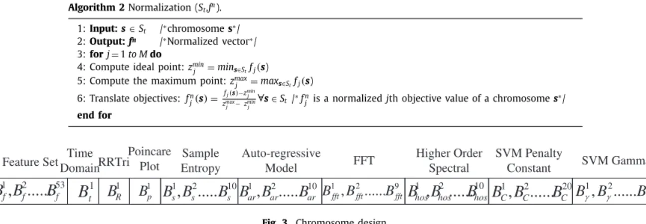
Algorithm2Normalization ( St,fn). 1: Input:s∈St / ∗chromosome s∗/ 2: Output:fn _/∗_Normalized_vector∗_/

3: forj=1 toMdo 4: Compute ideal point: zmin

j =mins∈Stfj(s) 5: Compute the maximum point: zmax

j =maxs∈Stfj(s) 6: Translate objectives: fn j(s)= fj(s)−zminj zmax j −zminj ∀

s∈St/ ∗fnj is a normalized jth objective value of a chromosome s∗/

endfor

Fig.3. Chromosome design.

proposed optimization algorithm is the chromosomes (Pareto opti-

mal solutions) that are belong to the front F1 of population Pt at

the end of the optimization.

Like in the original NSGA-III, two-layer reference points denoted

by the Zr_{are generated according to the Das and Dennis approach}

[42]. The initialization function takes the input parameters M, d1

and d2_{. The parent population}_P

t=0with population size N are also

randomly initialized. Then, two-point crossover and bit-ﬂip muta-

tion operators [29] are applied to Pt for producing the offspring

population Qtwith same population size N. The crossover and mu-

tation rates are determined by pcand pmrespectively.

After that, both population Pt and Qt are combined to formed

the population set Vt if generation t = 0. Otherwise, Vt only con-

sists of offspring population Qt. The population Vtsequentially goes

through the different stages of ﬁtness evaluation: HRV feature extraction, statistical performance evaluation, local search operation (LSO), duplication handling, prediction performance evaluation and

feature count evaluation. After the ﬁtness evaluation stage, Rt is

assigned Vt if generation t= 0. Otherwise, it consists of both Vt

and Pt. Then, all chromosomes in the population Rtare sorted into

different non-domination levels called fronts ( F1, F2,…) using the

dominance principle [25]. A new population St is constructed by

selecting individuals from different fronts ( F1, F2,…) until the size

of St is equal to N or greater than N for the ﬁrst time. The last

front ( Fi), which is assigned to St, is denoted by front Fl.

After that, Pt+1 is assigned St if the number of individuals in

St is exactly equal to N. Otherwise, Pt+1 is formed by the chro-

mosomes from front F1 up to Fl−1. In this case, they are still K

chromosomes need to be chosen from front Fl to ﬁll the Pt+1 un-

til | Pt+1| =N. The K chromosomes are chosen based on a series of

operations, which are adaptive normalization, association and nich-

ing. Except the normalization process in line 38, the procedures of

Algorithm1 from line 36 to 41 are same as the original NSGA-III

[25]. The mix-max normalization proposed by Yuan et al. [43] is

adopted to normalize the ﬁtness vector of every chromosome that

belong to set St. This process is summarized in Algorithm 2. The

procedure above is repeated until GENMAX. After that, the function

NDS-without-statistic-ﬁtness is applied to Ptin order to obtain the

solutions that belong to front F1.

3.5.2. Chromosomedesign

The structure of the proposed chromosome design is shown in

Fig. 3. The parameters and settings of the HRV based arrhythmia

prediction system are encoded into binary digits in the chromosome for optimization. The chromosome contains 135 bits that can be divided into 10 different segments.

The feature set segment is a 53-bit binary string that represents the selected HRV feature subset for a chromosome. Each bit in the

segment represents the feature selection status of one HRV feature. The bit “1” indicates selection while “0” represents the deletion of the speciﬁc feature from the feature set.

The last 2 segments are two 20-bit binary strings that represent

the encoded value of the parameters C and

γ

respectively for the

SVM model. The remaining seven segments, which are in the mid-

dle of a chromosome, represent various parameters and settings

for 7 different HRV feature extraction algorithms. Each of them is

explained in Table1.

Firstly, some of the binary digits in the Table1 are used to con-

trol the behavior of the heart rate correction, interpolation and signal detrending in the pre-processing stage of the baseline predic-

tion system (refer to Fig.2). Two separate bits are used to decide

whether the heart rate correction and detrending are performed on the HRV data respectively. As for the interpolation process, 2 different bits are used to control its behavior. One of them is used to determine either linear or cubic spline method is chosen to resample (interpolate) the HRV data. Another one is used to select the resampling frequency (either 4 Hz or 7 Hz).

The heart rate correction enabling status is important because the abnormal heart rate may contain the required information to

predict the arrhythmia event. In previous works [5–7], authors

counted the number of the occurrence of premature atrial contrac- tions (PACs) (a type of arrhythmia) in the ECG signal. The counted number was used to predict the PAF onset. The occurrences of the arrhythmia cause the abnormal heart rates in the time series HRV data. Therefore, the abnormal heart rate prior to the PAF onset may be useful for the PAF onset prediction. These abnormal heart rates are eliminated when the heart rate correction algorithm is applied. As for the interpolation and detrending, they can inﬂuence the en- ergy value of the power spectrum estimated by frequency domain algorithms.

For sample entropy analysis, the parameter values of the embedding dimension and tolerance distance are tuned by the proposed algorithm. Their values are set to integer range of 1–4 and ﬂoating point range of 0.1–0.5 respectively according to Lake et al.

[44]. Furthermore, the order of the auto-regressive (AR) model is

also set to integer range of 6–32 based on the investigation in

Anita et al. [38]. In both fast Fourier transform (FFT) and higher or-

der spectral (HOS) analysis, one type of temporal smoothing window function is selected among 8 different types of window function when the spectral analysis is performed. They are Rectangu- lar, Parzen, Hanning, Hamming, Blackman, Blackman Harris, Welch, and Barlette window. Furthermore, one bit denoted by “FFT seg-

mentation” in theTable1 is used to decide whether regular FFT or

Welch based FFT is chosen for performing the Fourier transform. Besides that, there is one extra bit that controls whether the PSD estimated by the AR and FFT are normalized to between 0 and 1 before the related HRV features are computed. Finally, the segmen-

(6)

Table1

Deﬁnition of the chromosome representation. Feature extraction

algorithm

Algorithm parameters Bit

length

Representation

1 Time domain • Heart rate correction enabling 1 bit • ‘0’ represents disabling while ‘1’ represents enabling of the ectopic beat correction.

2 RR Triangular Index • Heart rate correction enabling 1 bit • ‘0’ represents disabling while ‘1’ represents enabling of the ectopic beat correction.

3 Poincare plot • Heart rate correction enabling 1 bit • ‘0’ represents disabling while ‘1’ represents enabling of the ectopic beat correction.

4 Sample entropy • Heart rate correction enabling 1 bit • ‘0’ represents disabling while ‘1’ represents enabling of the ectopic beat correction.

• Embedding dimension 2 bit •Represent an integer value within the range of 1–4.

• Tolerance Distance 7 bit • Represent a ﬂoating value within the range of 0.1–0.5. 5 Auto Regressive (AR)

analysis

• Heart rate correction enabling 1 bit • ‘0’ represents disabling while ‘1’ represents enabling of the ectopic beat correction.

• Heart rate detrending

enabling 1 bit • ‘0’ represents disabling while ‘1’ represents enabling of the detrending.

• Interpolation method 1 bit • ‘0’ represents linear interpolation while ‘1’ represents cubic spline interpolation.

• Resampling frequency 1 bit • ‘0’ represents 4 Hz while ‘1’ represents 7 Hz.

• Order of model 5 bits • Represent an integer value within the range of 6–32.

• Normalization of AR spectrum 1 bit • ‘0’ represents no normalization while ‘1’ represents the spectrum is normalized by the maximum value of AR spectrum.

6 Fast Fourier Transform (FFT)

• Heart rate detrending enabling

1 bit • ‘0’ represents disabling while ‘1’ represents enabling of the detrending.

• Resampling frequency 1 bit • ‘0’ represents 4 Hz while ‘1’ represents 7 Hz.

• Temporal smoothing window function

3 Bit • Represents 8 types of symmetric smoothing window function.

• They are Rectangular, Parzen, Hanning, Hamming, Blackman, Blackman Harris, Welch and Barlette.

• FFT segmentation 1 Bit • ‘0’ represents normal FFT while ‘1’ represents welch based FFT with 50% data segment overlap.

• Normalization of FFT spectrum

1 bit • ‘0’ represents no normalization while ‘1’ represents the spectrum is normalized by the maximum value of FFT spectrum.

7 Higher Order Spectral (HOS) analysis

• Heart rate detrending enabling

1 bit • ‘0’ represents disabling while ‘1’ represents enabling of the detrending.

• Resampling frequency 1 bit • ‘0’ represents 4 Hz while ‘1’ represents 7 Hz

• Temporal smoothing window function

3 bit • Represents 8 types of symmetric smoothing window function.

• They are Rectangular, Parzen, Hanning, Hamming, Blackman, Blackman Harris, Welch and Barlette.

• Segmentation size 1 bit • ‘0’ represents 256 samples per segment while ‘1’ represents 512 samples per segment.

• Zero-padding size for the segmented data.

1 bit • ‘0’ represents the padding size is equal to segmentation size while ‘1’ represents twice of the segmentation size.

• Overlapping of the segmented data

1 bit • ‘0’ represents no overlapping in the segmented data while ‘1’ represents 50% overlap of the segmented data.

tation size, zero-padding size and overlapping of the segmented

data are also determined for the HOS analysis.

In the proposed chromosome design, the real number R of a

parameter that is encoded into binary string p (that has more than

1 bit) can be computed as:

R=minp+maxp−minp

2l₋₁ ×d (1)

where d is decimal value of binary string p, max p is maximum

value of parameter, min pis minimum value of parameter, l is

length of binary string p. The max p and min p for each real num-

ber parameter shown in Table1 are different. They are set accord-

ing to their minimum and maximum value of the speciﬁed integer

or ﬂoating point range. As for the SVM parameters C and

γ

, their

minimum and maximum value are set to 0.1 and 10 0 0 respectively.

3.5.3. Fitnessevaluationstage

The proposed ﬁtness evaluation stage consists of HRV feature extraction, statistical performance evaluation, local search operation, duplication handling, prediction performance evaluation and

feature count evaluation. Before entering the ﬁtness evaluation

stage, the duplicate chromosomes from population Qt are identi-

ﬁed by comparing them to all chromosomes from Pt and Qt. The

ﬁtness evaluation of these duplicate chromosomes are skipped and

reserved until they are modiﬁed by duplicate handling process

(line 19 of Algorithm 1). The detail of the duplicate chromosome

is explained in Section3.5.3.4 of this section.

3.5.3.1. HRVfeature extraction. During the HRV feature extraction

stage, for every chromosome that belong to the set Vt (referring to

Algorithm1), 53 HRV features in TableA.1 are extracted based on the decoded parameter values and settings. These parameter values

(7)

the feature extraction process, all HRV features are fed to statistical performance evaluation stage.

3.5.3.2. Statistical performance evaluation. The Mann–Whitney U

test is a non-parametric method used to test whether two in-

dependent samples of observations are drawn from the same or

identical distributions. Perez et al. [45] proposed a feature selec-

tion method called uFilter method, which is based on the Mann- Whitney U test, for single-objective optimization: feature selection. It is a standalone algorithm that evaluates the quality of a feature.

In their work, the statistic value denoted by wi was computed for

each feature. Then, top 20 features (with highest statistic values

wi in descending order) were selected to form a feature set. This

feature set was fed to the classiﬁcation models for training and

testing.

In this paper, the uFilter method is used to evaluate the HRV features of each chromosome for two optimization objectives: (1) to optimize the parameters and settings that belong to HRV feature extraction algorithms, and (2) to be used as an evaluation criterion in the local search operation (LSO). In the former objective, the optimization is achieved by minimizing the sum of the statistic values of all HRV features. It is computed as:

Sumofstatisticvalue=−

53

i=1

wi (2)

where wi is the absolute value of numerical difference between

ZNORMALand ZABNORMALfor ith feature (one of the 53 HRV features).

The algorithm that computes the wi,ZNORMAL and ZABNORMALcan be

found in [45]. The ZNORMALis the Z-indicator of feature values that

are extracted from HRV segments with the class label of “NOR-

MAL”, while the ZABNORMALis the Z-indicator of feature values ex-

tracted from HRV segments with the class label of “ABNORMAL”.

These two class labels are explained in Section3.1.

3.5.3.3. Localsearch operation(LSO). In this paper, the local search operation (LSO) is developed based on the hybrid feature selection

process of the simple GA proposed by Huang and Rong [30]. The

objectives of proposed LSO are: (1) to remove the non-signiﬁcant features from the feature subset in the chromosome so that only the good features are retained. (2) to maintain the minimum num-

ber of selected signiﬁcant features in the chromosome after the

removal process. The “significant feature” is the feature that can pass the evaluation criterion: two tailed Mann-Whitney U test at 20% significance level. Otherwise, it is referred as “non-significant feature”.

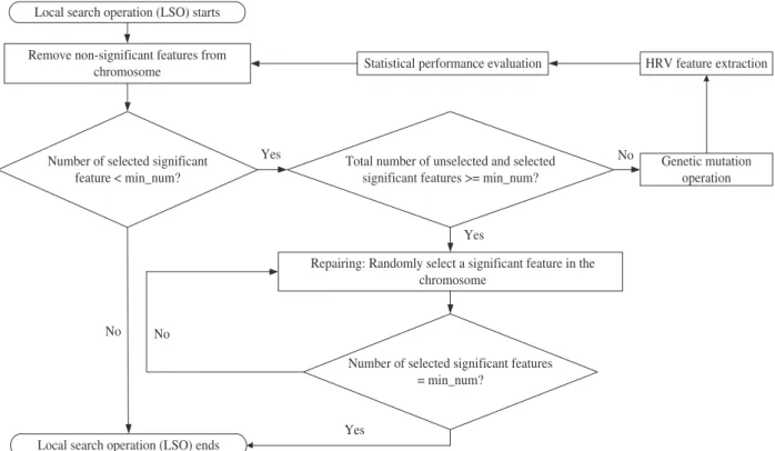
Fig. 4 shows the ﬂow chart of the proposed LSO. Initially, the

HRV features, which are selected within the feature subset seg-

ment of the chromosome, are examined. The non-signiﬁcant features are removed from the feature subset. This approach was used in [8] for manually removing the features that could not pass the U test before the simple GA was applied for feature selection.

After the above removal process, the chromosome is updated to reﬂect the changes. Then, the minimum number of selected significant features is evaluated. If the number equal or more than the

integer number of 3 (denoted by “min_num” in the Fig.4), the LSO

is ended. Otherwise, the handling process is started to increase the feature count to 3. In the handling process, the first step is to examine whether there is enough number of significant features for the selection. If it is enough, then one additional unselected significant feature is randomly selected and added to the feature subset. Otherwise, the chromosome goes through the mutation operation (genetic operation), HRV feature extraction stage and statistical evaluation stage again. Finally, the LSO is applied to this new chromosome. The handling process is repeated until the chromosome has same or more than the minimum number of significant features.

3.5.3.4. Duplication handling. Duplicate chromosome is the cre- ation of the same chromosome that has been evaluated before the current generation during the GA optimization process. It causes the computation wastage due to the redundant evaluation of du-

plicate chromosomes [46].

In this paper, the duplicate handling process is proposed to

handle (remove and replace) the duplicate chromosome. It is de-

veloped based on the method proposed by Saroj and Devraj [46].

They modiﬁed the duplicate chromosomes when there was a same chromosome exists in the one previous and the most current generations of the simple GA. Their results showed that the optimization performance of the simple GA was improved. Therefore, the

same concept is applied to the proposed optimization algorithm

in this paper because by default, the NSGA-III stores the previous population (population P) and current population (population Q) in one generation.

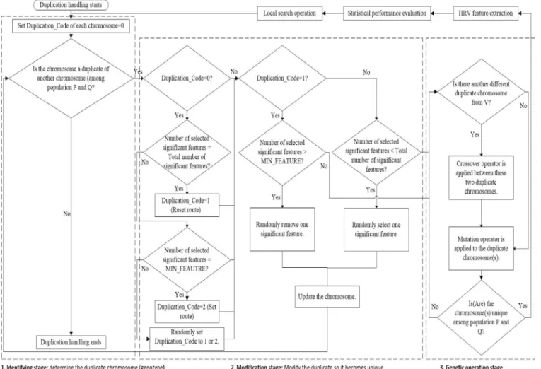
Fig. A.1 shows the ﬂow chart of the proposed duplicate han-

dling process. The algorithm can be divided into 3 main parts:

identifying stage, modiﬁcation stage, and genetic operation stage. In the identifying stage, the binary digit pattern of a chromosome

is compared against all the chromosomes in population Ptand Qt.

If its binary digit pattern is unique, the duplication handling process is ended. Otherwise, the chromosome is fed to the modiﬁca- tion stage.

In the modification stage, the content of the duplicate chromosome is modified so that it become unique among the population. When a chromosome enters this stage for the first time, its status represented by Duplication_Code is set to “0". Then, if the number of selected significant features in the feature subset is equal to total number of significant features (sum of both selected and unselected features in a chromosome), the duplicate chromosome is fed to reset route (by setting Duplication_Code to (1). If the number of selected significant features is equal to minimum number of features denoted by “min_num”, it will go to set route (by set-

ting Duplication_Code to (2). If neither of the conditions is met,

then it is randomly fed to either set route or reset route. In the reset route, if the number of selected significant features greater than min_num, then one of the significant features in the feature subset of the chromosome is removed. Otherwise, the chromosome is fed to genetic operation stage. In the set route, if the number of selected significant features is less than total number of signifi-

cant features, then one of the unselected signiﬁcant features is ran-

domly selected and added to the feature subset.

In the genetic operation stage, the ﬁrst step is to ﬁnd whether

there is another new but different duplicate chromosome exists.

If it exists, both crossover and mutation operators are applied to the modify both duplicate chromosomes. Otherwise, only mutation operator is applied to the current duplicate chromosome. The process in the genetic operation stage is repeated until the chromosome(s) becomes unique. Then, they are fed to HRV feature extraction stage, statistical performance evaluation, and local search operation. Finally, the duplicate handling process is repeated if nec- essary.

Several considerations are taken into account when developing the duplicate handling process. Firstly, the duplicate handling pro-

cess is placed after the LSO because the duplicate chromosomes

can be formed not only due to the genetic operation, but also due to the LSO. Secondly, HRV feature extraction process is avoided as

much as possible during the handling process because it is the

most computation intensive part of the algorithm. Therefore, the

modiﬁcation stage only alters the feature subset segment of the

duplicate chromosome. The parameters and settings of HRV fea-

ture extraction algorithms are only modiﬁed in genetic operation stage.

(8)

Remove non-significant features from chromosome

Number of selected significant feature < min_num?

Total number of unselected and selected significant features >= min_num? Yes

Repairing: Randomly select a significant feature in the chromosome

Number of selected significant features = min_num? No Yes Genetic mutation operation HRV feature extraction Statistical performance evaluation

No

No Local search operation (LSO) starts

Local search operation (LSO) ends

Yes

Fig.4. Flow chart of the local search operation (LSO).

3.5.3.5. Prediction performance evaluation. The prediction performance of each chromosome is evaluated. Initially, the chromosome is decoded in order to determine the selected feature subset, and

the values of SVM parameters (penalty constant C and gamma

γ

).

After that, the selected HRV features are taken from the training

dataset to train SVM model by using the decoded SVM parame-

ter values. The trained classifier is then evaluated with the testing dataset. Sensitivity (SEN), specificity (SPE), and accuracy (ACC) are used to measure the prediction performance. They are defined as follows: SEN= TP TP+FN (3) SPE=_T_NTN +FP (4) ACC= TP+TN TP+TN+FP+FN (5)

where TP is number of abnormal event (arrhythmia is occurred) that is correctly predicted, TN is number of normal event (No arrhythmia is occurred) that is correctly predicted, FN is number of arrhythmia event that is incorrectly predicted as normal event, FP is number of normal event that is incorrectly predicted as arrhythmia event.

10-fold cross validation is applied to evaluate the proposed

method. 10 ECG recordings (5 distant and 5 prior to onset of PAF event) are selected as testing set to measure the performance of classifier while remaining recordings (96 recordings) are used to train the classifier. This procedure is repeated over 10 times in order to cover entire database. In the 10th evaluation of 10-fold cross validation, training set contains 90 ECG recordings and testing set contains 16 ECG recordings. Then, average SEN, SPE and ACC are calculated as the measures for classification performance. Training set and testing set are subject independent (belong to different patient). Since it is well known that GA suffers from local optima issue, the optimization is repeated 5 times and the best results are selected for performance analysis.

3.5.3.6. Featurecount. In the proposed optimization algorithm, the feature count is deﬁned as the number of HRV features that are selected in a feature subset. The feature count is optimized by minimizing the ﬁtness value given by:

Feature count=

N

i=1

Fi (6)

where Fiis ‘1’ if ith feature is selected and ‘0’ if not selected, and

N is the total number of features (regardless the feature is selected

or not) in the feature set segment of the chromosome. The N is set

to 53 for this paper.

3.5.3.7. Non-dominated sorting (NDS). During the non-dominated

sorting (NDS) (line 28 of the Algorithm 1), the chromosomes

are divided and assigned to different sets (represented F1, F2,…)

[25] starting from F1. Each set Ficontains a group of solutions that

are not dominated to each other. The dominance operator denoted

by “_≺” is the standard symbol for representing the dominance rela-

tionship between two chromosomes. Assume that there is a min-

imization problem, the p≺q represents that the chromosome p is

said to strictly dominate another chromosome q, if and only if the

zi( p) ≤zi( q) for i=1, ..., M and zi( p) <zi( q) for at least one ﬁtness

function indexed by i, where M is total number of ﬁtness functions,

and zi( p) represents ith ﬁtness value of the chromosome p.

In this paper, ﬁve ﬁtness functions are proposed for the opti-

mization process. They are sum of statistic value ( Eq.(2)), predic-

tion sensitivity ( Eq.(3)), prediction speciﬁcity ( Eq.(4)), prediction

accuracy ( Eq.(5)), and feature count ( Eq.(6)). To ﬁt into the above-

described dominance operator ≺, some maximization ﬁtness func-

tions are turned into minimization ﬁtness function by multiplying

each of them with a ₋1.0. These functions are sensitivity, speci-

ﬁcity, and accuracy rate. The remaining ﬁtness functions are minimization functions by default.

The procedure of the NDS-without-statistic-ﬁtness (line 45 of the Algorithm1) is same as the process in NDS. However, there is one minor difference between them: the operation in dominance

(9)

Table2

Performance comparison between typical feature selection method and the proposed optimization method for PAF onset prediction.

Method Performance

SEN SPE ACC NF

Typical Method 88.7 66.0 77.4 4 Proposed Method 86.8 88.7 87.7 7

operator “≺”. The solutions in fronts Fi, which are produced by the

NDS-without-statistic-ﬁtness(), are non-dominated to each other

with respect to all proposed ﬁtness functions except the Eq.(2). In

contrast, the solutions produced by the NDS() are non-dominated to each other with respect to all ﬁtness functions. It is because this paper is interested in analyzing the prediction performance of the solutions.

4. Resultsanddiscussion

4.1. Performancecomparisonbetweenthetypicalmethodandthe proposedoptimizationalgorithm

In this section, the performance difference between the PAF onset prediction systems (solutions), which are optimized by the pro-

posed algorithm and the typical GA based feature selection method

respectively, is investigated.

The detail of the proposed optimization algorithm is described

by the Algorithm 1. The input parameters of the algorithm are

set as follows: N=212, pc=0.7, pm=0.1, M=5, d1=6, d2=0,

GENMAX=10 0 0. As for the typical GA based feature selection

(shown in Fig.1), the optimization methodology from [8] is em-

ployed for selecting the optimal feature subset and tuning the SVM parameters. The procedure of this method can be summarized as follows: Firstly, the same 53 HRV features are extracted based on the pre-deﬁned HRV parameter values and settings (which are ex-

plained in the Section3.2 and 3.3). After that, each HRV feature is

evaluated with two tailed Mann-Whitney U test. Only the features that can pass the U test at 20% significance level are selected and used to form a significant feature set. Finally, the simple GA feature selector is applied to this significant feature set for selecting

best feature subset. It should be noted that, unlike the proposed al-

gorithm in this paper, the HRV parameters and settings in typical method are not tuned. Therefore, the HRV feature extraction process is performed one time only since the parameter values and settings are same for every chromosome.

Each method is repeated 5 times with different initial populations. After that, the best solution represented by a chromosome

is selected from each method for performance analysis. Table 2

compares the prediction performance between the prediction systems that are optimized by typical feature selection method and

the proposed optimization algorithm respectively. With typical

method, the PAF onset prediction system achieves accuracy rate of 77.4%. The accuracy rate of the prediction system is improved by 10.3% when it is optimized by proposed algorithm. The prediction performance improvement is achieved because the proposed algorithm simultaneously optimizes all stages of the arrhythmia prediction system, while the typical method only optimizes the feature subset and SVM classiﬁer parameters.

The higher prediction performance can also be attributed to

more number of HRV features can pass the Mann–Whitney U test.

Table 3 shows the HRV features that able to pass the two tailed U test at 5%, 10% and 20% signiﬁcance levels for typical method and proposed method. In typical method, only 10 HRV features can pass the U test up to 20% signiﬁcance level. In contrast, the number is improved to 32 when the proposed optimization algorithm

is used, and majority of them pass the 5% signiﬁcance level. The improvement is achieved because the proposed optimization algorithm explicitly tunes the HRV parameter values and settings for improving the statistic value of each HRV feature by minimizing

the ﬁtness value of Eq.(2). Furthermore, in Table3, it is observed

that all signiﬁcant features from the typical method also re-appear as the signiﬁcant features from the proposed method, except the

HH-WCOB( f2m). Finally, TableA.2 shows the difference between the

pre-deﬁned and optimized values for the parameters and settings of HRV feature extraction algorithms.

When the number of features that pass the U test increases,

the NSGA-III has opportunity to explore and evaluate more combi-

nation of HRV features [8]. This leads to higher possibility in ob-

taining the optimal feature set with higher accuracy. However, only 10 HRV features are available for typical method while 32 HRV features are available for the proposed optimization algorithm.

In addition to the prediction performance, Table 2 shows that

although the optimal subset selected by typical method has lower

(better) feature count than proposed method, but at the expense of

signiﬁcant lower accuracy rate. The typical method selects 4 features (out of 10 HRV features) to form the feature subset, which reduces the feature count by 60%. The selected features are AR-LF, LL-H2, LL-H3, ROI-H2. In contrast, the proposed method selects 7 features (out of 32 HRV features), which reduces the feature count by 78%. The selected features are NN50, pNN50, SampEn, SD2, AR-

LF, LL-H1, ROI-WCOB ( f2m), and all of them can pass the U test at

5% signiﬁcance level.

4.2.Trade-off betweenperformancemetrics

In the typical feature selection method based on the simple GA (with weighted sum approach), each GA run returns a single so-

lution. Therefore, the typical method in Section 4.1 only gives a

solution that has highest accuracy rate. In contrast, with the pro-

posed NSGA-III based optimization algorithm, multiple solutions

that have different degree of trade-off between the performance metrics can be obtained in a single optimization run.

Table 4 shows the prediction sensitivity, speciﬁcity, accuracy rate and feature count of the Pareto optimal solutions. These solutions are obtained from the same optimization run that gives the

best solution in Table2. It should be noted that these solutions are

only a portion of the Pareto optimal solutions given by the output of Algorithm 1. These solutions are selected for analysis because they have highest prediction sensitivity at certain speciﬁcity rate, or vice versa.

Table4 shows that the sensitivity of the solutions can be improved, but at the expense of lower specificity rate. For example, from solution 1 to 10, the sensitivity rate increases from 43.4 to 100%, while the specificity rate decreases from 96.2% to 26.4%. On the other hand, the accuracy rate increases from solution 1, peaks at 5, and then decreases until solution 10. Unlike sensitivity and specificity, the changes in accuracy rate does not show either in- creasing or decreasing trend. It is because the increment (or decre-

ment) in sensitivity rate may outpace the decrement (or incre-

ment) in speciﬁcity rate.

The solution 5, which has the highest accuracy rate among the

Pareto optimal solutions, is used for comparison in Table 2 and

benchmarking in Table5. Furthermore, the accuracy rate of solu-

tion 1, 2 and 10, which have the best sensitivity or specificity rate, are significant lower than 80% (that is achieved by other solutions in Table4). It shows that even the sensitivity can be improved over certain threshold value, a significant trade-off is needed in specificity, or vice versa.

(10)

Table3

HRV features that able to pass the two tailed U test up to 20% signiﬁcance level for PAF onset. Signiﬁcance Level HRV feature

typical method Proposed method

5% AR-LF, FFT-LF, LL-H2, LL-H3, LL-H4, HH-WCOB( f1m), HH-WCOB( f2m)

SDRR, RMSSD, NN50, pNN50, SampEn, SD1, SD2, AR-LF, AR-HF, FFT-LF, FFT-HF, LL- Mave, LL- Pave, LL-H1, LL-H2, LL-H3, LL-H4, LH-P1, LH- Mave, LH- Pave, LL-H1, ROI-P1, ROI-P2, ROI- Mave, ROI- Pave, ROI-WCOB( f2m), ROI-H1

10% – LL-P1, LH-P2

20% FFT-HF, LL- Mave, ROI-H2 HH-H1, ROI-WCOB( f1m), ROI-H2

Table4

Trade-off between sensitivity, speciﬁcity, accuracy rate and feature count.

Solution SEN (%) SPE (%) ACC (%) Feature count

1 43.4 96.2 69.8 4 2 45.3 94.3 69.8 4 3 75.5 92.5 84.0 7 4 83.0 90.6 86.8 6 5 86.8 88.7 87.7 7 6 90.6 81.1 85.9 5 7 92.5 79.3 85.9 5 8 94.3 71.7 83.0 3 9 98.1 60.4 79.3 5 10 100.0 26.4 63.2 5

Fig.5. Average number of the duplicate chromosomes for 5 optimization runs without handling at generation t.

4.3.Duplicatechromosomes

The results in this section show that high number of dupli-

cates chromosomes are formed when NSGA-III is adapted for optimization in this paper. It wastes the computation resource and increases the optimization time when these duplicate chromosomes

are re-evaluated. Fig. 5 shows the average number of duplicates

for successive NSGA-III generations when they are not handled by

the duplicate chromosome handling process. The average number is computed by summing and averaging the number of duplicates in each generation of 5 different optimization runs.

First of all, the line denoted by “Duplicate 1" is the number of duplicate chromosomes found by comparing each chromosome to

other chromosomes within the population Pt only. For example, if

they are 4 chromosomes that have same binary pattern within the

population Pt, the count is increased by 3 (4 −1). Fig.5 shows that

the average number increases from 0 to around 60 within 50 generations, and then remains around that number (within range of

±10) in the following generations. It represents approximately 28%

of the chromosomes in population Pt that has total size of 212.

Another line denoted by “Duplicate 2" is the number of duplicate

chromosomes found by comparing each chromosome in population

Qtto all the chromosomes in population Pt after the LSO in ﬁtness

evaluation stage. The count is increased by 1 if there are two same

chromosomes between two populations in a generation. Fig.5 also

shows that this number also increases rapidly within 100 generations.

With the proposed duplicate handling process, the number de-

noted by “Duplicate 1" becomes zero for all generations (zero

duplicate), which means all the chromosomes in population Pt

and Pt+1 are unique. Although the number denoted by “Dupli-

cate 2" remains same, the related duplicates are not re-evaluated.

It is because they are formed during the normal genetic opera-

tion (line 8 of Algorithm 1), and they are identiﬁed before en-

tering the fitness evaluation stage. Their fitness re-evaluations are skipped until modified by the duplicate handling process (line 19 of Algorithm1).

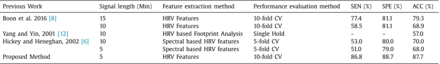
4.4. Benchmarking

Table 5 shows the benchmarking results of our proposed method against the previous works that use less than 15 min of HRV signal for prediction. Our proposed method achieves prediction accuracy rate of 87.7% by using the shortest HRV signal length

among all previous works: 5 min only. Furthermore, this accu-

racy rate outperforms all previous works that in Table 5. Boon

et al. [8] achieved accuracy rate of 79.3% but used longest sig-

nal length with 15 min. Their accuracy rate was reduced to 68.9%

when 10 min signal is used. Yang and Yin [12] employed 10 min

signal and it achieved the lowest accuracy rate among previous

works with 57%. Finally, Hickey and Heneghan [6] only achieved

accuracy rate of 68% and 70% for 5 min and 10 min respectively. Table5

Benchmarking of proposed method against previous works using less than 15 min of signal length.

Previous Work Signal length (Min) Feature extraction method Performance evaluation method SEN (%) SPE (%) ACC (%)

Boon et al. 2016 [8] 15 HRV Features 10-fold CV 77.4 81.1 79.3

10 HRV Features 10-fold CV 58.5 81.1 68.9

Yang and Yin, 2001 [12] 10 HRV based Footprint Analysis Single Hold – – 57.0

Hickey and Heneghan, 2002 [6] 10 Spectral based HRV features 5-fold CV 53.0 80.0 70.0

5 Spectral based HRV features 5-fold CV 51.0 79.0 68.0

Proposed Method 5 HRV Features 10-fold CV 86.8 88.7 87.7

(11)

Table6

Prediction performance of previous works that used 30 min signal for prediction.

Previous Work Feature extraction method Performance evaluation

method

SEN (%) SPE (%) ACC (%)

Zong et al. [7] Number and timing of PACs Single Hold – – 80.0

Hickey and Heneghan [6] PACs detection and Spectral based HRV features 5-fold CV 79.0 72.0 75.0

Thong et al., [5] PACs Analysis Single Hold 89.00 91.00 90.0

Costin et al. [9] HRV features and Morphological Variability of QRS complexes of ECG

Single Hold 89.3 89.4 89.4

Mohebbi and Ghassemian [10] HRV features Single Hold 96.2 93.1 94.5

Cheskonov [11] HRV based spectral features Single Hold 72.7 88.2 80.0

Lynn and Chiang [13] HRV based Return Map and Poincare Plot features Single Hold – – 64.0

In Table6 , the prediction performances of the previous works using 30 min data (either ECG or HRV signal depending on feature extraction method) are summarized. When compared to these previous works, our proposed method outperforms all of them except

[5,9,10]. Our method is 1.7% lower than Costin et al. [9], 2.3% lower

than Trans et al. [5], 6.8% lower than the highest accuracy achieved

by Mohebbi and Ghassemian [10]. Finally, the feature count of the

proposed method is improved. The proposed method only uses

7 HRV features, which is signiﬁcantly lower than 12 HRV features

in best previous work [10].

Although our proposed method does not outperform them

[5,9,10], they are several factors that need to be taken into con- sideration during the comparison. Firstly, their methods required longer duration of HRV signal for prediction. In contrast, the sig-

nal length is reduced by 83.33% (from 30 minto 5 min) in our

method. Furthermore, they only employed single hold out validation method – it is well known that separating samples to single training and testing set can bias the performance of classiﬁer. In this paper, 10-fold cross validation method, which is better method than single hold-out, is employed to estimate prediction accuracy

of proposed work. The K-fold method is considered better than

hold-out method because K-fold method can reduce the overﬁt-

ting problem of trained classiﬁer model [31], and more suitable to

evaluate algorithm with small sample size of dataset [47]. Further-

more, Tran et al. [5] did not use HRV analysis for prediction, and

they also needed to specify both recordings belong to same sub- jects before classifying the data. The proposed method does not require this extra step of specifying both recordings. Costin et al.

[9] also used non-HRV analysis based features called morphological variability features that are extracted from QRS complexes in ECG signal. In contrast, the proposed method employs HRV analysis based features only.

5. Conclusion

In this paper, a paroxysmal atrial ﬁbrillation (PAF) prediction

method based on HRV analysis and NSGA-III is proposed. The proposed PAF onset prediction method achieves accuracy with 87.7% that outperforms all previous works that use less than 30 min signal for prediction. It is achieved even with HRV signal length being reduced from typical 30 min to 5 min (a reduction of 83%).

The improvements are achieved by proposing the NSGA-

III based multi-objective optimization algorithm that can

simultaneously optimizes all stages of the PAF onset prediction

system. Furthermore, the trade-off between prediction sensitivity

and speciﬁcity is analyzed, in which the results show that the

sensitivity can be improved at the expense of lower speciﬁcity.

Mann–Whitney U test is also used as the ﬁlter method to examine

the statistical signiﬁcance of the features before they can be

selected to form the feature subset. Finally, a duplicate handling process is proposed to reduce the computation wastage due to the duplicate chromosomes.

As for limitation of this work, the proposed method still needs

improvement in order to achieve same or higher accuracy rate than

best work [10]. The proposed prediction method is also limited by

a small sample size of real data from patients. Therefore, our result may not represent the true characteristic of the general PAF population. Furthermore, due to small sample size, the proposed algorithm is not evaluated with the testing data not included in the cross-validation process. As a result, evaluation with such testing set will be performed after we acquire larger sample size in future. Finally, the optimization process takes hours on single per- sonal computer because multiple ﬁtness evaluation processes are performed on each NSGA-III solution. However, it is not an issue in practice since the proposed optimization process is run single time only to ﬁnd the best prediction model before real-world de- ployment.

Hence, the following future works are planned to improve our

method. Firstly, more types of HRV feature extraction algorithm

that are reviewed in [37] can be used for prediction. Furthermore,

different ﬁlter methods such as analysis of variance, t-test and mu-

tual information can be used to evaluate the features. The impact of different methods on the optimization performance can be analyzed and compared to U test in this paper. Finally, the duplication handling process can be improved so that it records all the chromosomes that have been evaluated in all previous generations.

Then, the history record is used to determine the duplication status

of a chromosome in the most recent generation. Such approach is

employed in the simple GA [48] to completely eliminate the dupli-

cate chromosome, but at the expense of higher memory and computation resource. Another future work is extending and applying the proposed optimization algorithm to other HRV research problems such as prediction of ventricular tachyarrhythmia onset and detection sleep apnea. It is applicable as long as the classiﬁcation

model is similar to baseline model in Fig.2, with some changes in