Modeling of an activated sludge process for effluent prediction—a comparative study using ANFIS and GLM regression

Modeling of an activated sludge process for effluent

prediction

—

a comparative study using ANFIS and GLM

regression

Dauda Olurotimi Araromi&Olukayode Titus Majekodunmi &

Jamiu Adetayo Adeniran&Taofeeq Olalekan Salawudeen

Received: 29 January 2018 / Accepted: 25 July 2018 / Published online: 1 August 2018 #Springer Nature Switzerland AG 2018

Abstract In this paper, nonlinear system identification

of the activated sludge process in an industrial waste-water treatment plant was completed using adaptive neuro-fuzzy inference system (ANFIS) and generalized linear model (GLM) regression. Predictive models of the effluent chemical and 5-day biochemical oxygen demands were developed from measured past inputs and outputs. From a set of candidates, least absolute shrinkage and selection operator (LASSO), and a fuzzy brute-force search were utilized in selecting the best combination of regressors for the GLMs and ANFIS models respectively. Root mean square error (RMSE) and Pearson’s correlation coefficient (R-value) served as metrics in assessing the predicting performance of the models. Contrasted with the GLM predictions, the ob-tained modeling results show that the ANFIS models provide better predictions of the studied effluent vari-ables. The results of the empirical search for the domi-nant regressors indicate the models have an enormous potential in the estimation of the time lag before a

desired effluent quality can be realized, and preempting process disturbances. Hence, the models can be used in developing a software tool that will facilitate the effec-tive management of the treatment operation.

Keywords Wastewater treatment process modeling .

Predictive models . ANFIS . Fuzzy exhaustive search . GLM regression . LASSO regularization

Introduction

Tightening environmental constraints have made it in-creasingly important for chemical process plants to be operated efficiently and in an environmentally friendly manner. Although several strategies have been put in place to combat the menace of water pollution; waste-water treatment still remains a major global challenge for process industries, as the performance of any waste-water treatment plant (WWTP) is affected by a distinct combination of some physical, chemical, and biological factors (Belanche et al.2000; Mjalli et al.2007; Singh et al.2010).

Important water quality parameters frequently used to assess the performance of WWTPs include 5-day biochemical oxygen demand (BOD), chemical oxygen demand (COD), and total suspended solids (TSS). Fre-quent monitoring of these parameters helps plant oper-ators preempt process disturbances and, hence, maintain environmental balance. This task often involves labori-ous and expensive laboratory analyses (Dupuit et al. 2007). Therefore, the determination of wastewater https://doi.org/10.1007/s10661-018-6878-x

D. O. Araromi

:

:

:

Department of Chemical Engineering, Ladoke Akintola University of Technology, Ogbomoso P.M.B. 4000, Nigeria e-mail: [email protected]

O. T. Majekodunmi

Department of Chemical Engineering, Izmir Institute of Technology, 35430 Izmir, Turkey

J. A. Adeniran

Department of Chemical Engineering, University of Ilorin, Ilorin P.M.B. 1515, Nigeria

treatment indices using predictive models could help in a safe and cost-effective management of the treatment process (Belanche et al.1999; Mjalli et al.2007; Singh et al.2010; Nadiri et al.2018).

Wastewater treatment processes are highly nonlinear: involving strongly coupled physical, chemical, and bi-ological activities. Hence, predictive models developed from mechanistic approaches are usually dimensionally complex, and the solutions are intractable, computation-ally intensive, and time-consuming (Mjalli et al.2007; Araromi et al.2014; Nadiri et al.2018). Also, several assumptions often applied to simplify the resulting mod-el introduce some degree of uncertainty which signifi-cantly affects the precision (Gontarski et al. 2000; Gernaey et al.2004).

Contrariwise, soft computing techniques such as artificial neural network (ANN) and adaptive neuro-fuzzy inference system (ANFIS) have been found to be efficient in the formulation of high-performing models of complex nonlinear processes from histor-ical data (El-Din and Smith2002; Hamed et al.2004; Mjalli et al.2007). Singh et al. (2010) applied linear and nonlinear techniques to model a biological WWTP based on the effluent BOD and COD. The techniques are: partial least squares regression (PLSR), multivariate polynomial regression (MPR), and ANN. The authors concluded the nonlinear modeling techniques (MPR and ANN) provided bet-ter predictions.

Nasr et al. (2012) also developed an ANN model to predict the performance of a biological WWTP in Egypt using BOD, COD, and TSS as the character-istic parameters. The authors indicated the model sufficiently describes the nonlinear behavior of the WWTP and can be used as a valuable assessment tool by plant operators and management. In Mjalli et al. (2007), ANN models for the prediction of the effluent BOD, COD, and TSS of a local WWTP were formulated. The model was incorporated into a computer program to help operators monitor the WWTP performance and ensure compliance with discharge regulations. Pai et al. (2009) compared the performance of ANN and ANFIS in the predic-tion of the effluent suspended solids and COD of a hospital WWTP. It was reported that ANFIS outper-forms ANN in the prediction exercises.

Though ANN is a robust tool in modeling highly nonlinear processes, it has some undesirable de-merits. They are (1) the choice of network structure

and the problem of poor generalizations associated with its incorrectness; (2) the knowledge of the model is stored in synaptic weights and cannot be easily interpreted; and (3) large amount of data is needed to generate an adequate model. However, recent studies have proved that ANFIS overcomes these limitations, but the choice of model inputs still poses a challenge in ANFIS modeling (Passino and Yurkovich 1998; Hamed et al. 2004; Pai et al. 2009; Suh et al. 2009; Pai et al. 2011; Nasr et al. 2012).

Generalized linear model (GLM) regression is another peculiar class of nonlinear modeling tech-niques which has found applications in wastewater process modeling (Dürrenmatt and Gujer 2012). It uses random components to specify the distribution of the response variable and a smooth invertible linearizing link function to transform its expectation to a function of the regressors (Hardin and Hilbe 2007). GLM is an extension of the familiar regres-sion models that make use of normal distribution as conditional distribution for response variables. Non-normal distributions used to extend the usual regres-sion framework include Poisson, gamma, inverse-Gaussian, and binomial (McCullagh and Nelder 1989).

In previously published works, the model inputs were mostly selected arbitrarily. However, to obtain optimum results, it might help to make the choice via appropriate empirical methods (Tomić et al. 2018). For instance, Ahmadi et al. (2018) investigated the influence of model inputs selected using different combinations of methods which include principal component analysis, gamma test, and correlation model on the performance of a BOD model. The authors reported the choice of inputs have significant effects on the model prediction.

In this study, a procedure for the nonlinear dynamical system identification of a biological wastewater treat-ment process using ANFIS and GLM regression is described and exemplified. Models for the prediction of the effluent BOD and COD were both developed from past inputs and output variables. For each model, a brute-force search also known as exhaustive search was employed in selecting the most adequate combina-tion of the variables for the ANFIS models while a penalized regression method termed least absolute shrinkage and selection operator (LASSO) was used for the GLMs.

Materials and methods

The case study

The data used in this study was collected from the WWTP of Seven-Up Bottling Company in Lagos, Nigeria. This company is one of the largest beverage manufacturing industries in the country. The compa-ny produces different brands of soft drinks which are widely consumed in the country. The plant de-pends on a large volume of water in its daily oper-ations which include, but not limited to, the prepa-ration of feedstock and purification of packaging bottles.

The process wastewater contains oil, solid objects, suspended particles, dissolved chemicals, and organic substances. The wastewater is disposed of in the treat-ment operation cycle before discharged into the main water body in the environment. The treatment objective is to remove or reduce objectionable materials to a level that conforms to environmental regulations and stan-dards which limits the COD and 5-day BOD of effluent discharges into surface waters and drainages to 30 and 6 mg/l, respectively.

The treatment process consists of three main stages, viz. physical, chemical, and biological treatment pro-cesses. The biological treatment step is an activated sludge system where dissolved biodegradable organic matter is degraded by micro-organisms to an acceptable and ecologically safe limit. This is a typical example of a process whose dynamics is difficult to fully comprehend and manage due to perturbations in flow, organic load, and concentration of micro-organisms per unit time (Pons et al. 1999; Gernaey et al. 2004; Moral et al. 2008; Cristea et al.2009).

Five-day BOD and COD are the organic content indicators of the wastewater in this case study. These parameters are monitored through sampling and labora-tory analyses before and after treatment. Some of the analyses involve the use of hazardous reagents such as mercury sulfate, chromium trioxide, sulfuric acid, and potassium dichromate. They are exacting and requiring sophisticated laboratory equipment and gadgets. Also, the determination of COD can take few hours while BOD 5 days. For these reasons, accurate predictive models developed from the historical data can facilitate real-time monitoring and effective management of the WWTP. Hence, it will be of important use in maintain-ing environmental balance and ensurmaintain-ing the safeness of

water bodies (Dürrenmatt and Gujer 2012; Heddam et al.2016).

This study is primarily concerned with the activated sludge system. Three hundred fifty-nine datasets were collected over the period of a year, as seasonal changes were considered important in capturing possible varia-tions in the studied variables (Mjalli et al.2007; Nasr et al. 2012; Heddam et al. 2016). The collected data include the influent and effluent BOD and COD record-ed on a daily basis, and cover the peak (dry season) and the lowest period (rainy season) of the company’s prod-ucts demand.

Data preprocessing

To produce models that satisfactorily map-out the pro-cess behavior, the data was prepropro-cessed to eliminate some likely unusable information which are probably introduced into the WWTP database as a result of mea-surement errors (Oliveira-Esquerre et al.2002; Hamed et al.2004; Rustum and Adeloye2007; Yel and Yalpir 2011; Tangirala2015). Firstly, the dataset was subjected to a statistical tool to sort out and remove outliers which were classified as data-points lying outside ± 2σ, stan-dard deviation of the group mean (Mjalli et al. 2007). This procedure reduced the dataset to 324 data-points.

Also, for adequate process representation, the pres-ence of noise in the data is undesirable as it causes non-smoothing in the data trend which is counterproductive. Thus, a data smoothing technique was applied to reduce noise and normalize gaps caused by the removal of the outliers (Rustum and Adeloye2007). In the smoothing process, each data-point was replaced with the average of the neighboring data-points defined within a span using moving average filter which is mathematically expressed as:

ysð Þ ¼i 1

2Nþ1ðy iðþNÞ þy iðþN−1Þ þ…þy ið−NÞÞ ð1Þ

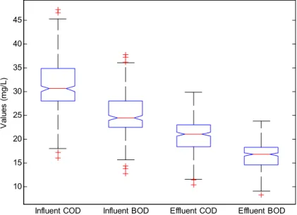
In Eq. (1),ys(i) is the smoothed value of thei-th data-point, Nis the number of neighboring data-points on either side of ys(i), and 2N+ 1 is the span. Most re-searchers use three-, four-, or five-point moving aver-ages (span) (Mjalli et al.2007). In this study, five-point moving averages (span = 5) was used because it gave satisfactory result when compared to others. The statis-tical information of the preprocessed dataset is presented in Fig.1.

Brief description of system identification

This is the process of building models of dynamic systems from observed input–output data. It involves the use of the past inputs and outputs, known as regres-sors, as model inputs (Passino and Yurkovich 1998; Tangirala2015). A linear mapping of this form is de-fined as:

y kð Þ ¼∑q_i¼1θaiy kð −iÞ þ∑pi¼0θbiu kð −i−1Þ ð2Þ

In Eq. (2),y(k) and u(k) are the system output and input variables at time interval k≥0 respectively. The number of the past output and input variables used are represented by q and p, respectively. The parameters associated with the past output and input variables are

θaandθb, respectively. When Eq. (2) is expressed in a matrix notation, it becomes:

y kð Þ ¼ f xð Þ ¼jθ θTx ð3Þ Where, x¼½y kð −1Þ;…;y kð −qÞ;u kð Þ;…;u kð −p−1ÞT θ¼ θa1;…;θaq;θb0;…θbq T ) ð4Þ In Eqs. (3) and (4),xis the regression vector, andθis the vector of unknown parameters to be estimated. Each vector is of dimensionNx1 where N=q+p+ 1. System identification involves adjusting θ making use of the information contained in the observed data until the error between the predicted and observed values is reduced to an acceptable tolerance. Fuzzy identification follows the same procedure by utilizing the predefined regression vector x, but with functional capabilities which enable it to achieve more accurate identification of nonlinear systems than the linear map defined in Eq. (2) (Passino and Yurkovich1998; Araromi et al.2014).

ANFIS architecture

Basically, neuro-fuzzy system, which only supports Takagi–Sugeno–Kang (TSK) model, is a fuzzy infer-ence system (FIS) constructed in the framework of a neural network. It employs the easy interpretability and expansiveness of fuzzy logic and the robust learning ability of artificial neural networks as it extracts fuzzy rules from observed data into a rule-base (Passino and Yurkovich1998; Guillaume2001; Karray and De Silva 2004; Mingzhi et al.2009; Nadiri et al.2018). A rule in

a first-order TSK (with consequent linear function) is as expressed in Eq. (5). pth:IFX1is Ap1ANDX2is A p 2…ANDXnis ApnTHENOp ¼αp 0þαp1X1þ…αpnXn ð5Þ In Eq. (5),Xiis thei-thinput linguistic variable of the

p-thrule. The corresponding linguistic value isAp_i andn

is the number of input linguistic variables.Ap_i is linked to a membership function (MF) μ_Ap

ið ÞXi . In each rule consequent, Op denotes the output of the inference process, and αp₀;…;αp_n are Sugeno parameters. For a zero-order TSK, each rule consequent is a constant (αp₀) as other Sugeno parameters are set to zero. Moreover, each rule in ANFIS has unity weight and one output.

Fig.2shows the structure of a first-order TSK model formulated as a five-layer feed-forward network. The model in the figure has two inputs, four rules, and an output which is determined by weighted average defuzzification method. Each layer is a step in a fuzzy identification process and their functionality is described as follows (Guillaume 2001; Karray and De Silva 2004):

Layer 1: Fuzzification

Each node i, characterized by a MF, converts the crisp inputs into membership values.

O1_i ¼μ_Ap

ið ÞX ð6Þ

Layer 2: Rule nodes

To evaluate the degree of fulfillmentWpof each rule, T-norm, and T-conorm operators are used to express the AND and OR connectives respectively. An example of a T-norm operation is:

Wp¼μApið Þ⨂X1 μA p

jð ÞX2 ; i¼1;2;j¼1;2;p

¼1;…;4 ð7Þ

Layer 3: Normalization

The normalized firing strength of the p-th rule is calculated as the ratio of its firing strength to the sum of all rules firing strengths.

Wp¼ Wp

∑4

p¼1Wp

ð8Þ Layer 4: Rule consequent

These nodes evaluate the consequent of each fuzzy rule. The values of the consequents are multiplied by normalized firing strengths.

O4_p¼WpOp¼Wp αp0þα p 1X1þαp2X2 ð9Þ Layer 5: Summation

The final output is calculated as the sum of all in-coming signals. O5¼∑4_p¼1Wp αp0þα p 1X1þαp2X2 ð10Þ Regressors formulation and selection

In this work, two multi-input single-output models were identified from the collected process data. One is for the prediction of the effluent COD (model 1) while the other is for the effluent BOD (model 2). In each case, four past outputs and six past inputs, organized into three groups, were considered as model input candidates as expressed in Eq. (11) whereu1(k) andu2(k) depicts the influent BOD and COD respectively. And the effluent BOD or COD is represented byy(k). x¼ uy k1ððk−−ijÞÞ;; 11≤≤ij≤≤46 u2ðk−jÞ 8 < : ð11Þ

It is quite difficult to determine how to select exog-enous variables for adequate model approximation and the search for the combination of the input candidates which influences the output the most is a major chal-lenge (Passino and Yurkovich1998; Ahmadi et al.2018;

Tomićet al.2018). A fuzzy brute-force search was used to select the ANFIS models inputs while LASSO was used for the GLM regressors. The search space is expo-nential in size and the task is to findx∈Xwhich satisfies a condition ψ. This exhaustive search method iterates through all the elements in the search space, testing every possible candidate solution. It builds an ANFIS model for each combination, trains it for one epoch, and reports its performance.

Since it is logical that the regressors should not exclusively be from any of the process inputs or outputs, one regressor each was selected from the three sets highlighted in Eq. (11) (Passino and Yurkovich1998; Tangirala2015). This step was separately performed for the two models and 144 combinations were generated in each case as shown in Eq. (12):

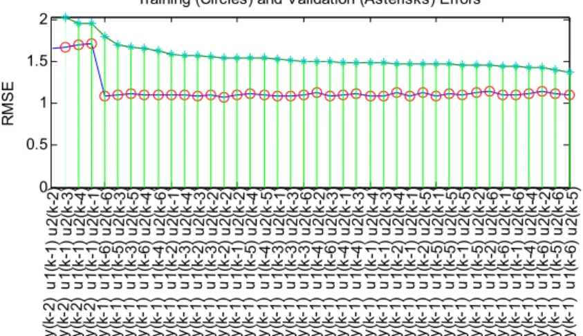
4

1C*61C *61C¼144 ð12Þ Fuzzy exhaustive search algorithm identifies the combination with the least training RMSE. But in order to obtain models with minimal error and no over-fitting, two other criteria were considered simultaneously. They are low validation RMSE and relatively low positive difference between the training and validation RMSE. Figs. 3 and 4 show the exhaustive search results for ANFIS models 1 and 2 respectively. Incidentally, the combination of regressorsy(k−1),u1(k−6), and u2(k

−5) satisfied these conditions for both models and thus stands out as the required regression vector. A rule in a first-order Sugeno model considered in this study is:

10 15 20 25 30 35 40 45

Influent COD Influent BOD Effluent COD Effluent BOD

Va lu e s ( m g /L )

Fig. 1 Statistical features of the modeled data

p_th:IFy kð −1ÞisAp₁ANDu1ðk−6ÞisAp2ANDu2ðk−5ÞisAp3THENOp ¼αp 0þα p 1y kð −1Þ þα p 2u1ðk−6Þ þα3pu2ðk−5Þ ð13Þ

For clear observation, only the combinations having comparatively low RMSE values are reported in the plots. In Fig.3, it is observed that the aforesaid combi-nation has the least validation error and a relatively low training error. The difference between the error values, which is illustrated as the distance between both points on the plot, is comparatively low. This scenario is also observed in the regressor selection process for ANFIS model 2 (Fig.4).

Notably, the identified regressors reveal the time interval between a change in the process inputs and the first significant change in the response. In case of a process disturbance and tightening environmental con-straints, this information can aid the WWTP operators in approximating the time needed to realize a set treatment quality before the treated wastewater is discharged into the environment. Eq. (13) shows that at any instant in time (day,k) the value of the effluent five-day BOD or COD, y(k), can be obtained from y(k−1), u1(k−6),

and u2(k−5) before new measurements are obtained. Since the measurement process takes time, this implies that by employing the described model inputs selection method, it is possible to approximate future effluent conditions based on measured past variables. The plant managers can also detect potential process disturbances, at least, a day earlier. In such cases, a number of acti-vated sludge process variables, such as the hydraulic or sludge retention time and mixing rate, can be adjusted to control the situation and avoid a likely shutdown. Fuzzy identification

Neuro-fuzzy systems are developed in two successive stages: structure and parameter learning. In the structure learning stage, a set of input–output numerical data is partitioned to define the rules structure. Each partition represents a rule and their boundaries overlap. Common partitioning techniques include grid-type and clustering. In grid partitioning, withninputs andkinput MFs, the number of rules is kn. Though the number of rules increases exponentially, grid portioning is effective in extracting all the rules for a small number of inputs (Guillaume2001; Karray and De Silva2004).

Grid partitioning was used in this study and two input MFs were affixed to each regressor. The number of MFs to be associated with each model input was determined by trial-and-error (Mjalli et al.2007; Jang1993). It was observed that any value higher than two increased the models’complexity and returned a very high training

and validation error. Thus, the number of rules generat-ed is kn= 23= 8. Figure 5 shows the adopted FIS structure.

In the second stage, the values of the connection weights and MFs parameters are adjusted and optimized using learning algorithms. The hybrid learning algorithm proposed by Jang (1993) was adopted in this work: back-propagation method which is based on gradient-descent optimization technique was employed to tune the antecedent parameters while least squares method was used for the consequent part.

The preprocessed data was divided into two: one-half was used for model training and the other for validation. Because correct ANFIS model specifications are deter-mined empirically, the effects of five different input MF types on the predicting performance of zero- and first-order Sugeno model structures was examined (Jang and Sun1995; Guillaume2001; Pai et al.2011). The essence was to identify the model specifications required to realize a satisfactory performance. The considered input MFs are presented in Table1.

Generalized linear model (GLM) regression with LASSO regularization

GLM regressions extend linear model regressions by relaxing the assumption of linearity in the parameters with the introduction of a link function and the use of error distributions other than normal distribution. As shown in Eq. (14), the model is a function of meanμ with a linear combinationxβformed from regressorsx

and coefficient vectorβ. The mean μiof the response variableyiis modeled as a monotonic nonlinear trans-formation of a linear function (ηi) of the regressors. For each set of observation, the linearizing invertible link functiong(·) transforms the expected value of the re-sponseμi=E(yi) to the linear predictor such thatμi=

g−1(ηi) =E(yi) (McCullagh and Nelder1989; Hardin and Hilbe2007).

gð Þ ¼μ_i η_i¼β₀þβ₁xi1þβ2xi2þβ3xi3þ…

þβkxik ð14Þ

The choice of the linearizing transformation which is partially separated from the distribution of the response is an advantage in GLM regression. Common GLM link functions include: identity, natural logarithm, inverse-square, inverse, square root, logit (sigmoid), and probit. The identity link function, as the name implies, returns

its argument unchanged such that μi=g− 1

(ηi) =ηi=

E(yi).

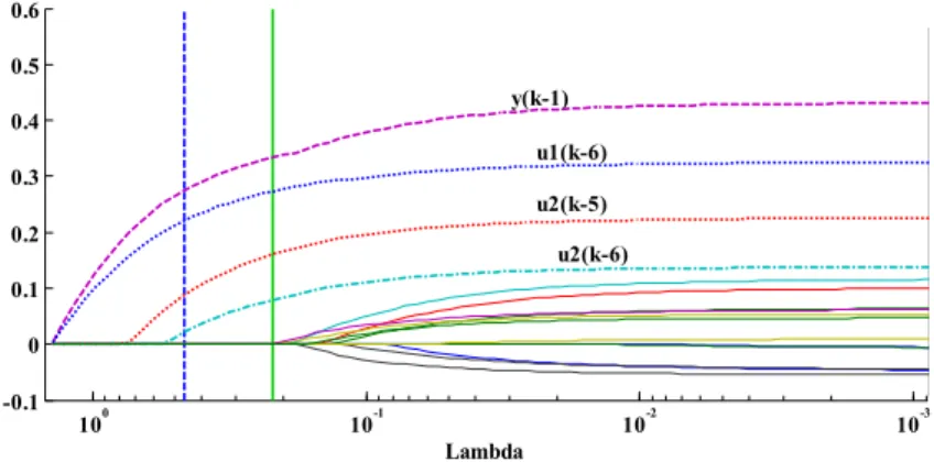
Least absolute shrinkage and selection operator (LASSO) is a regularization method used with GLM regression to identify and select dominant regressors amongst redundant ones, and produce shrinkage esti-mates with potentially low prediction errors than the regular least squares. LASSO approach minimizes the prediction error subject to a non-differentiable constraint presented in terms of the L1-norm of the coefficients (Tibshirani1996). A nonnegative regularization param-eterλ, known as penalty, is introduced to constrain the size of the estimated coefficients and solve the objective function in Eq. (15) whereNrepresents the number of data-points,β0the intercept andβthe p-vector of the coefficients.Dis the estimated expected deviance of the model applied to new data as evaluated by cross-valida-tion. Asλincreases, the number of nonzero elements in

βdecreases. min β0; β 1 NDðβ0;βÞ þλ∑ p j¼1 βj ð15Þ

Tibshirani (1996) proposed ak-fold cross-validation algorithm for the estimation of the prediction error in order to compute the bestλ. In this method, LASSO is indexed in terms ofλand the prediction error is calcu-lated over a range of values ofλfrom 0 to 1 inclusive. The value ofλwhich gives the least prediction error is selected. This method is often used for small parameters vector space. Tenfold cross-validation was used in this work. Figure 6 shows the cross-validated deviance of the LASSO fit. It is a plot of the absolute deviance againstlog λ. The broken vertical line with the blue circle indicates theλwith the minimum deviance while the longest continuous vertical line with the green circle locates the minimum deviance plus one standard deviation. 0 0.5 1 1.5 2 y (k -2) u 1(k -1 ) u2 (k -2) y( k-2 )u 1 (k -1) u 2 (k-3 ) y (k -2) u 1 (k-1 ) u2 (k -4 ) y(k -2 )u 1 (k -1) u 2 (k-1 ) y (k -1) u 1 (k-6 ) u2 (k -6 ) y(k -1 )u 1 (k -5) u 2 (k-3 ) y (k -1) u 1 (k-3 ) u2 (k -5 ) y(k -1 )u 1 (k -6) u 2 (k-4 ) y (k -1) u 1 (k-4 ) u 2(k -6 ) y (k-1 ) u1 (k -2) u 2 (k-1 ) y (k -1) u 1( k-3 ) u2 (k -4) y (k-1 ) u1 (k -2) u 2 (k-3 ) y (k -1) u 1 (k-3 ) u2 (k -2 ) y (k-1 ) u1 (k-2) u 2 (k-2 ) y (k -1) u 1(k -1 ) u2 (k -2) y (k-1 ) u1 (k -5) u 2 (k-4 ) y (k -1) u 1( k-4 ) u 2(k -5 ) y (k-1 ) u1 (k -3 )u 2 (k -1) y (k -1) u 1 (k-3 ) u 2(k -3 ) y( k-1 ) u1 (k -3 )u 2 (k -6) y (k -1) u 1 (k-4 ) u2 (k-2 ) y( k-1 ) u1 (k-6) u 2 (k-3 ) y (k -1) u 1 (k-4 ) u 2(k -1) y (k-1 ) u1 (k -4) u 2 (k-3) y (k -1 )u 1 (k-1 ) u 2(k -4 ) y (k-1 ) u1 (k -1 )u 2 (k -3) y (k -1 )u 1 (k-2 ) u 2(k -4) y (k-1 ) u1 (k -1 )u 2 (k -1) y (k -1 )u 1 (k-2 ) u 2 (k-5 ) y (k-1 ) u1 (k -5 )u 2 (k -1) y( k-1 )u 1 (k-5 ) u 2(k -5 ) y (k-1 ) u1 (k -1 )u 2 (k-5) y(k -1 )u 1 (k -5) u 2(k -2 ) y (k -1) u 1(k -2 )u 2 (k-6) y (k -1 )u 1 (k-6 ) u 2(k -1 ) y (k-1 ) u 1(k -1 )u 2 (k -6) y (k -1 )u 1 (k -4) u 2 (k-4 ) y (k-1 ) u 1(k -6 )u 2 (k -2) y( k-1 )u 1 (k-5 ) u 2(k -6 ) y (k -1) u 1(k -6 ) u2 (k -5)

Training (Circles) and Validation (Asterisks) Errors

RM

S

E

Fig. 3 Selection of regressors for ANFIS model 1 0 0.5 1 1.5 y (k -2) u 1 (k-1 ) u2 (k -2 ) y (k-2 )u 1 (k -1) u 2 (k-1 ) y (k -2 ) u 1 (k-1 ) u2 (k -3 ) y(k -2 ) u1 (k -1) u 2 (k-4 ) y (k -1 ) u 1 (k-5 ) u2 (k -3 ) y(k -1 ) u1 (k -3) u 2 (k-5 ) y (k -1 ) u 1 (k-6 ) u2 (k -6 ) y (k-1 )u 1 (k -6) u 2 (k-4 ) y (k -1 ) u 1 (k-4 ) u2 (k -6 ) y (k-1 ) u1 (k -2 )u 2 (k-1 ) y (k -1) u 1 (k-2 ) u2 (k -3 ) y (k-1 ) u1 (k -3) u 2 (k-4 ) y (k -1) u 1 (k-3 ) u 2(k -2 ) y (k-1 ) u1 (k -1) u 2 (k-2 ) y (k -1) u 1 (k-5 ) u 2(k -4 ) y (k-1 ) u1 (k -3) u 2 (k -1) y (k -1 )u 1 (k-2 ) u 2(k -2 ) y (k-1 ) u 1(k -4 )u 2 (k -5) y (k -1 )u 1 (k -3) u 2(k -6 ) y (k -1) u 1(k -1 )u 2 (k -1) y(k -1 )u 1 (k -3) u 2(k -3 ) y (k-1 ) u 1(k -4 )u 2 (k -2) y(k -1 )u 1 (k -6) u 2 (k-3 ) y (k -1 ) u 1(k -2 )u 2 (k -4) y (k-1 )u 1 (k -1) u 2 (k-3 ) y (k -1 ) u 1 (k-4 ) u2 (k -1 ) y (k-1 ) u1 (k -2) u 2 (k-5 ) y (k -1 ) u 1 (k-1 ) u2 (k -4 ) y (k-1 ) u1 (k -4) u 2 (k-3 ) y (k -1) u 1 (k-5 ) u2 (k -1 ) y (k-1 ) u1 (k -5) u 2 (k-5 ) y (k -1) u 1 (k-1 ) u2 (k -5 ) y (k-1 ) u1 (k -5 )u 2 (k -2) y (k -1 )u 1 (k-2 ) u 2(k -6 ) y (k-1 ) u1 (k -6 )u 2 (k -1) y (k -1 )u 1 (k-1 ) u 2(k -6 ) y (k-1 ) u 1(k -4 )u 2 (k -4) y (k -1 )u 1 (k-6 ) u 2(k -2 ) y (k-1 ) u 1(k -5 )u 2 (k -6) y(k -1 )u 1 (k -6) u 2 (k-5 )

Training (Circles) and Validation (Asterisks) Errors

RM

S

E

Fig. 4 Selection of regressors for ANFIS model 2

Figure 7 displays the nonzero model coefficients plotted as a function oflogλ. Each curve on the plot represents each of the 16 model input candidates (regressors) highlighted in Eq. (11). As observed, LAS-SO sets more coefficients to zero while few nonzero ones remain asλincreases. The regressors having non-zero model coefficients at the minimum deviance plus one standard deviation point arey(k−1),u1(k−6),u2(k

−5),and u2(k−6). The LASSO regularization was also separately performed for both models and the same regressors suggested by the fuzzy search, with the ex-ception ofu2(k−6), were obtained.

In the estimation of the GLMs, the responses were considered to have inverse-Gaussian distribution. The link functions used are identity, logarithmic, square root, inverse, and square. The inverse-Gaussian distribution,

otherwise known as Wald distribution, can be used to model nonnegative positively skewed data. Though this distribution emanated from the theory of Brownian mo-tion, it has been utilized in modeling different phenom-ena (Jablonski et al. 2013). The density function is presented in Eq. (16) whereμis the expected value of the response and λ is the inverse of the dispersion parameter. p yð Þ ¼ ffiffiffiffiffiffiffiffiffiffi λ 2πy3 s exp − λ 2μ2_yðy−μÞ 2 fory>0 ð16Þ

Models predicting performance metrics

RMSE and Pearson’s correlation coefficient (R-value) were used to statistically assess the predicting perfor-mance of the models: how well the predicted data ap-proximates the modeled raw data. These metrics are mathematically expressed as:

RMSE¼ ffiffiffiffiffiffiffiffiffiffiffiffiffiffiffiffiffiffiffiffiffiffiffiffiffiffiffiffiffiffiffiffiffiffiffiffiffiffiffiffiffiffiffiffi ∑n i¼1 Xobsv;i−Xpred; i 2 n s ð17Þ R−value¼ ∑ n i¼1 Xobsv;i−Xobsv ∙ Xpred; i−Xpred ffiffiffiffiffiffiffiffiffiffiffiffiffiffiffiffiffiffiffiffiffiffiffiffiffiffiffiffiffiffiffiffiffiffiffiffiffiffiffiffiffiffiffiffiffiffiffiffiffiffiffiffiffiffiffiffiffiffiffiffiffiffiffiffiffiffiffiffiffiffiffiffiffiffiffiffiffiffiffiffiffiffiffiffiffi ∑n i¼1 Xobsv;i−Xobsv 2 ∙∑n i¼1 Xpred; i−Xpred 2 r ð18Þ

WhereXobsvis the measured or observed value,Xpredis the predicted value, andnis the number of observations.

Xobsv and Xpred are the means of the observed and predicted values respectively. The reliability of the mod-el depends on the closeness of the RMSE to zero andR -value to + 1 (Gontarski et al.2000; Mjalli et al.2007; Pai et al.2011; Dürrenmatt and Gujer2012; Heddam et al. 2016; Oke et al.2017).

Fig. 5 Adopted ANFIS model structure

Table 1 Mathematical expressions of the considered MFs

Input MF Notation Membership value μAp_ið ÞX h i Triangular trimf max min X−ai bi−ai; X−ai bi−ai ;0 Trapezoidal trapmf max min X−ai bi−ai;1; X−ai bi−ai ;0

Generalized bell gbellmf ₁ 1þX−ci

ai

2bi

Gauss (one-sided) gaussmf exp−

X−ci 2σi 2

Gauss (two-sided) gauss2mf exp−

X−c_i

σi 2

Results and discussion

ANFIS modeling

As earlier stated, model 1 is the predictive model of the effluent COD while model 2 denotes that of the effluent BOD. Table2 presents the predicting performance of ANFIS model 1 for different combinations of input and output MFs. Although the least difference between the training and validation errors was achieved whentrimf

andlinearwere used as the MFs and the corresponding RMSE values are also relatively low; it is observed that the R-value (0.947) is a bit lower than that obtained whengbellmfandconstantwere used as the input and output MFs respectively. Also, thegbellmfandconstant

MF combination produced the highestR-value (0.948). Figure8 shows how the errors change as the training proceeds. It illustrates that convergence was achieved for both the training and validation errors before the 200th epoch. The resulting training (1.130) and valida-tion RMSE (1.302) are also comparatively low and the positive difference between both does not suggest

model over-fitting. Therefore, the combination of

gbellmf and constant MF types suitably identify the relationship that exists between the modeled variables for ANFIS model 1.

The predicting performances of ANFIS model 2 for different combinations of input and output MFs are presented in Table3. From the table, the highestR-value (0.947) was realized in four different modeling scenar-ios. Two of these cases are significant because they gave lower validation errors. They are trimfand linear, and

gbellmfandconstantMFs combination, but the positive difference between the training (0.899) and validation RMSE (1.041) for thegbellmfandconstantMFs com-bination is lower when compared to that obtained in the

trimf and linear MFs combination. This implies less over-fitting in the resulting model, thus, making it the model configuration with the best predicting perfor-mance for ANFIS model 2. The training progress for this case is presented in Fig.9. It shows the errors also converged before the 200th epoch. This informs that the data was not over-fitted and, hence, the produced model generalizations are reliable.

10-4 10-3 10-2 10-1 100 100 120 140 160 180 200 220 240 260 280 300 Lambda De v ia n ce

Fig. 6 Tenfold cross-validated LASSO fit 10-3 10-2 10-1 100 -0.1 0 0.1 0.2 0.3 0.4 0.5 0.6 Lambda y(k-1) u1(k-6) u2(k-5) u2(k-6)

Fig. 7 Trace plot of coefficients fits by LASSO

GLM regression

The influence of different transformations (link func-tions) on the predicting performance of the two GLMs was studied. The result of the performance evaluation is presented in Table4. The maximumR-value (0.637) and

the least errors were realized when no transformation (identity link) was applied to the responses. This is consistent with that obtained in ANFIS modeling, where the same model specifications yielded the best predicting performance for both models. The GLM regression is expressed as:

y kð Þ ¼β₀þβ₁∙y kð −1Þ þβ₂∙u1ðk−6Þ þβ3∙u2ðk−5Þ þβ4∙u2ðk−6Þ þβ5∙y kð −1Þ 2_þβ

6∙u1ðk−6Þ2

þβ7∙u2ðk−5Þ2þβ8∙u2ðk−6Þ2þβ9∙y kð −1Þ∙u1ðk−6Þ þβ10∙y kð −1Þ∙u2ðk−5Þ þβ11∙y kð −1Þ∙u2ðk−6Þ

þβ12∙u1ðk−6Þ∙u2ðk−5Þ þβ13∙u1ðk−6Þ∙u2ðk−6Þ þβ14∙u2ðk−5Þ∙u2ðk−6Þ ð19Þ

Table 2 Predicting performance using different MFs for ANFIS model 1

Input MF RMSE R-value

Output function Output function

Constant Linear Constant Linear

Training Validation Training Validation

trimf 1.164 1.310 1.129 1.309 0.946 0.947 trapmf 1.152 1.336 1.097 1.359 0.945 0.946 gbellmf 1.130 1.302 1.094 1.361 0.948 0.946 gaussmf 1.178 1.329 1.092 1.355 0.944 0.946 gauss2mf 1.173 1.341 1.112 1.372 0.944 0.945 0 100 200 300 400 500 600 700 800 900 1000 1.1 1.15 1.2 1.25 1.3 1.35 1.4 1.45 1.5 1.55 Epoch Numbers RM S E

Training (green) and Validation (red) error curve

Fig. 8 Training progress for ANFIS model 1

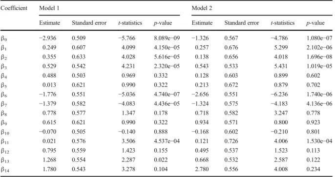
For both models, the estimated coefficients and their statistics are presented in Table5. At 5% signif-icance level, the intercept (β0) and all the LASSO selected regressors, except u2(k−6), are significant, as the p-values≪0.05. This observation is also in agreement with the fuzzy brute-force search result wherey(k−1),u1(k−6),and u2(k−5) were selected as the most influential regressors. However, the R -values and RMSE -values reported in Table 4 are undesirable. When these values are compared to those obtained in ANFIS modeling, it can be provi-sionally said that the ANFIS models perform better than the GLMs.

Significance of the results

The results obtained in this work are consistent. The same regressors were identified in the fuzzy exhaustive search and LASSO regularization processes and identi-cal specifications produced the desired predicting per-formance in both models and modeling approaches. This is largely due to the modeled data structure, and affirms that the reliability of a black-box model hinges on the correctness of the data. It is noteworthy that appropriate model specifications are determined empir-ically which is a time-consuming process for higher number of inputs as it necessitates testing different com-binations of the variables before arriving at one that

Table 3 Predicting performance using different MFs for ANFIS model 2

Input MF RMSE R-value

Output function Output function

Constant Linear Constant Linear

Training Validation Training Validation

trimf 0.918 1.046 0.893 1.043 0.946 0.947 trapmf 0.934 1.074 0.864 1.086 0.944 0.946 gbellmf 0.899 1.041 0.860 1.081 0.947 0.947 gaussmf 0.930 1.060 0.861 1.078 0.945 0.947 gauss2mf 0.950 1.101 0.903 1.101 0.941 0.944 0 100 200 300 400 500 600 700 800 900 1000 0.85 0.9 0.95 1 1.05 1.1 1.15 1.2 1.25 Epoch Numbers RM S E

Training (green) and Validation (red) error curve

Fig. 9 Training progress for ANFIS model 2

gives the desired model performance. In this study, three input variables were used to adequately model a highly nonlinear behavior and the adopted model structure achieved this within a reasonably short simulation time, circumventing the curse of dimensionality peculiar to grid-partitioning techniques in ANFIS modeling (Guillaume 2001; Karray and De Silva 2004; Jang 1993).

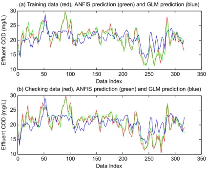
How good is a fit? One obvious metric is how close it is to the measured data-points. For visual inspection, fits of the measured data and model predictions of the effluent COD and BOD are presented in Figs.10and 11respectively. For both model training and validation

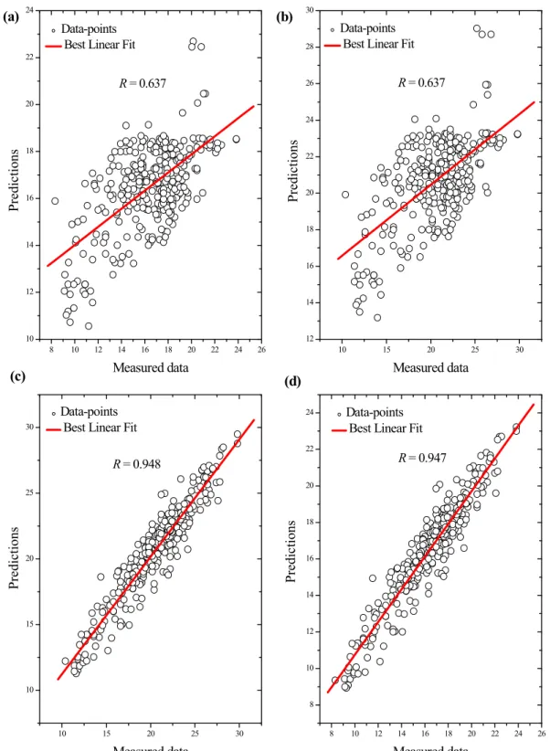
datasets, the figures show the ANFIS predictions are closer to the corresponding measured values than the GLM predictions. Figure 12a, b, c, d illustrates the degree of linear relationship between the measured data and the corresponding predictions of GLM 1, GLM 2, ANFIS model 1, and ANFIS model 2 respectively. The linear fits reveal that the measured data and ANFIS predictions are in satisfactory agreement. These show the ANFIS models outperform the GLMs. The results also illustrate that wastewater treatment processes, such as this case study, are highly nonlinear and cannot be effectively modeled using mechanistic approaches or linear model structures (Oliveira-Esquerre et al. 2002;

Table 4 GLM regression results

Transformation Model 1 R-value Model 2 R-value

RMSE RMSE

Training Checking Training Checking

Identity 2.895 3.042 0.637 2.307 2.415 0.637

Natural logarithm 2.915 3.083 0.631 2.319 2.441 0.632

Inverse 2.984 3.193 0.615 2.369 2.517 0.619

Square 2.929 3.090 0.629 2.338 2.466 0.626

Square root 2.899 3.055 0.635 2.309 2.422 0.635

Table 5 GLMs estimated coefficients and their statistics

Coefficient Model 1 Model 2

Estimate Standard error t-statistics p-value Estimate Standard error t-statistics p-value

β0 −2.936 0.509 −5.766 8.089e−09 −1.326 0.567 −4.786 1.080e−07 β1 0.249 0.607 4.099 4.150e−05 0.257 0.676 5.299 2.102e−06 β2 0.355 0.633 4.028 5.616e−05 0.138 0.656 4.018 1.696e−08 β3 0.529 0.542 4.231 2.320e−05 0.543 0.533 5.431 1.019e−05 β4 0.488 0.503 0.969 0.332 0.128 0.603 0.899 0.602 β5 0.013 0.621 0.990 0.322 0.213 0.672 0.879 0.702 β6 −1.776 0.551 −5.036 4.740e−07 −2.656 0.551 −6.236 1.740e−06 β7 −1.379 0.582 −4.083 4.436e−05 −1.324 0.575 −4.183 4.136e−06 β8 0.778 0.577 1.347 0.178 0.718 0.582 3.247 0.778 β9 0.615 0.621 0.990 0.322 0.934 0.571 0.800 0.923 β10 −0.070 0.505 −0.140 0.888 −0.168 0.602 −0.210 0.801 β11 0.021 0.576 3.506 4.537e−04 0.121 0.726 4.006 1.530e−04 β12 0.795 0.559 1.423 0.155 0.495 0.537 1.523 0.113 β13 1.268 0.554 2.287 0.022 0.668 0.532 2.587 0.122 β14 1.780 0.543 3.278 0.104 2.780 0.556 4.008 0.234

Gernaey et al.2004; Moral et al.2008; Singh et al.2010; Heddam et al.2016; Oke et al.2017).

Conclusions

The application of mechanistic approaches in identify-ing the behavior of nonlinear processes is taskidentify-ing. But ANFIS has yet proved its capability as an efficient

model approximating tool by adequately mapping-out a highly nonlinear biological wastewater treatment pro-cess based on previously measured inputs and output values of the studied variables. ANFIS predicted the process outputs with greater accuracy when compared with the GLM regression models. The data used in the study were pretreated to remove outliers and reduce noise as the predictive performance of black-box models depends on the exactness of data. Also, the influential

0 50 100 150 200 250 300 350 10 15 20 25 30

(a) Training data (red), ANFIS prediction (green) and GLM prediction (blue)

Data Index E ff luent C O D (m g/ L) 0 50 100 150 200 250 300 350 10 15 20 25 30

(b) Checking data (red), ANFIS prediction (green) and GLM prediction (blue)

Data Index E ff lue nt C O D ( m g/ L)

Fig. 10 Comparison of the model predicted and measured effluent COD values: (a) training data; (b) validation/checking data

0 50 100 150 200 250 300 350 5 10 15 20 25

(a) Training data (red), ANFIS prediction (green) and GLM prediction (blue)

Data Index Ef fl u e n t BO D ( m g /L ) 0 50 100 150 200 250 300 350 5 10 15 20 25

(b) Checking data (red), ANFIS prediction (green) and GLM prediction (blue)

Data Index E ff lu ent B O D ( m g/ L)

Fig. 11 Comparison of the model predicted and measured effluent BOD values: (a) training data; (b) validation/checking data

regressors identified indicate there are time lags in the treatment process. This is understandable as wastewater

undergo both chemical and biological changes before new process conditions are established. Therefore, the 8 10 12 14 16 18 20 22 24 26 10 12 14 16 18 20 22 24 10 15 20 25 30 12 14 16 18 20 22 24 26 28 30 10 15 20 25 30 10 15 20 25 30 8 10 12 14 16 18 20 22 24 26 8 10 12 14 16 18 20 22 24 Pre dic tions Measured data Data-points Best Linear Fit

R = 0.637

Data-points Best Linear Fit

R = 0.637 Pre dic tions Measured data Data-points Best Linear Fit

R = 0.948

Data-points Best Linear Fit

R = 0.947 Pre dic tions Measured data

(d)

(c)

(b)

(a)

ANFIS models can also serve as a reliable tool to estimate the time required to achieve a set treatment performance and also preempt process disturbances. The described modeling approach can be extended to other WWTPs as it would help the decision makers in effectively managing the plant operations in order to ensure the effluent quality consistently complies with the discharge regulations.

Acknowledgements The authors would like to acknowledge the support of Seven-Up Bottling Company, Lagos, Nigeria for re-leasing the data used.

References

Ahmadi, A., Fatemi, Z., & Nazari, S. (2018). Assessment of input data selection methods for BOD simulation using data-driven models: a case study. Environmental Monitoring and

Assessment, 190, 239.

https://doi.org/10.1007/s10661-018-6608-4.

Araromi, D. O., Sonibare, J. A., & Emuoyibofarhe, J. O. (2014). Fuzzy identification of reactive distillation for acetic acid recovery from wastewater. Journal of Environmental

Chemical Engineering, 2, 1394–1403. https://doi.

org/10.1016/j.jece.2014.05.008.

Belanche, L. A., Valde, J. J., Comas, J., Roda, I. R., & Poch, M. (1999). Towards a model of input–output behaviour of waste-water treatment plants using soft computing techniques.

Environmental Modelling & Software, 14, 409–419.

https://doi.org/10.1016/S1364-8152(98)00102-9.

Belanche, L., Valde, J. J., Comas, J., Roda, I. R., & Poch, M. (2000). Prediction of the bulking phenomenon in wastewater treatment plants.Artificial Intelligence in Engineering, 14, 307–317.https://doi.org/10.1016/S0954-1810(00)00012-1. Cristea, V., Pop, C., & Agachi, P. S. (2009). Artificial neural

networks modelling of PID and model predictive controlled wastewater treatment plant based on the benchmark simula-tion model no. 1.Computers & Chemical Engineering.

https://doi.org/10.1016/S1570-7946(09)70197-X.

Dupuit, E., Pouet, M. F., Thomas, O., & Bourgois, J. (2007). Decision support methodology using rule-based reasoning coupled to non-parametric measurement for industrial waste-water network management.Environmental Modelling &

Software, 22, 1153–1163. https://doi.org/10.1016/j.

envsoft.2006.05.025.

Dürrenmatt, D. J., & Gujer, W. (2012). Data-driven modeling approaches to support wastewater treatment plant operation.

Environmental Modelling & Software. https://doi.

org/10.1016/j.envsoft.2011.11.007.

El-Din, A. G., & Smith, D. W. (2002). A neural network model to predict the wastewater inflow incorporating rainfall events.

Water Research, 36, 1115–1126.https://doi.org/10.1016

/S0043-1354(01)00287-1.

Gernaey, K. V., van Loosdrecht, M., Henze, M., Lind, M., & Jørgensen, S. B. (2004). Activated sludge wastewater

treatment plant modelling and simulation: state of the art.

Environmental Modelling & Software, 19, 763–783.

https://doi.org/10.1016/j.envsoft.2003.03.005.

Gontarski, C. A., Rodrigues, P. R., Mori, M., & Prenem, L. F. (2000). Simulation of an industrial wastewater treatment plant using artificial neural networks. Computers &

Chemical Engineering, 24, 1719–1723. https://doi.

org/10.1016/S0098-1354(00)00449-X.

Guillaume, S. (2001). Designing fuzzy inference systems from data: an interpretability-oriented review.IEEE Transactions

on Fuzzy Systems, 9, 426–443. https://doi.org/10.1109

/91.928739.

Hamed, M. M., Khalafallah, M. G., & Hassanien, E. A. (2004). Prediction of wastewater treatment plant performance using artificial neural networks. Environmental Modelling &

Software, 19, 919–928. https://doi.org/10.1016/j.

envsoft.2003.10.005.

Hardin, J.W. & Hilbe, J.M. (2007). Generalized linear models and extensions. Texas: Stata Press.

Heddam, S., Lamda, H., & Filali, S. (2016). Predicting effluent biochemical oxygen demand in a wastewater treatment plant using generalized regression neural network based approach: a comparative study.Environmental Processes, 3, 153–165.

https://doi.org/10.1007/s40710-016-0129-3.

Jablonski, A., Barszcz, T., Bielecka, M., & Breuhaus, P. (2013). Modeling of probability distribution functions for automatic threshold calculation in condition monitoring systems.

Measurement, 46, 727–738. https://doi.org/10.1016/j.

measurement.2012.09.011.

Jang, J.-S. R. (1993). ANFIS—adaptive network-based fuzzy inference system.IEEE Transactions on Systems, Man, and

Cybernetics, 23, 665–685. https://doi.org/10.1109

/21.256541.

Jang, J.-S. R., & Sun, C.-T. (1995). Neuro-fuzzy modeling and control.Proceedings of the IEEE, 83, 378–406.https://doi. org/10.1109/5.364486.

Karray, F. O., & De Silva, C. W. (2004). Soft computing and

intelligent systems design: theory, tools and applications.

England: Pearson Education.

McCullagh, P., & Nelder, J. A. (1989).Generalized linear models. New York: Chapman & Hall.

Mingzhi, H., Jinquan, W., Yongwen, M., Yan, W., Weijiang, L., & Xiaofei, S. (2009). Control rules of aeration in a submerged bio-film wastewater treatment process using fuzzy neural networks. Expert Systems with Applications, 36, 10428– 10437.https://doi.org/10.1016/j.eswa.2009.01.035. Mjalli, F. S., Al-Asheh, S., & Alfadala, H. E. (2007). Use of

artificial neural network black-box modeling for the predic-tion wastewater treatment plants performance. Journal of

Environmental Management, 83, 329–338. https://doi.

org/10.1016/j.jenvman.2006.03.004.

Moral, H., Aksoy, A., & Gokcay, C. F. (2008). Modeling of the activated sludge process by using artificial neural networks with automated architecture screening. Computers &

Chemical Engineering, 32, 2471–2478. https://doi.

org/10.1016/j.compchemeng.2008.01.008.

Nadiri, A. A., Shokri, S., Tsai, F. T. C., & Moghaddam, A. A. (2018). Prediction of effluent quality parameters of a waste-water treatment plant using a supervised committee fuzzy logic model.Journal of Cleaner Production, 180, 539–549.

Nasr, M. S., Moustafa, M. A., Seif, H. A., & El Kobrosy, G. (2012). Application of artificial neural network (ANN) for the prediction of El-Agamy wastewater treatment plant per-formance—Egypt.Alexandria Engineering Journal, 51, 37– 43.https://doi.org/10.1016/j.aej.2012.07.005.

Oke, E.O., Jimoda, L.A., & Araromi, D.O. (2017). Determination of biocoagulant dosage for water clarification using devel-oped neuro-fuzzy network integrated with user interface based calculator. Water Science and Technology: Water Supply, ws2017241,https://doi.org/10.2166/ws.2017.241. Oliveira-Esquerre, K. P., Mori, M., & Bruns, R. E. (2002).

Simulation of an industrial wastewater treatment plant using artificial neural networks and principal component analysis.

Brazilian Journal of Chemical Engineering, 19, 365–370.

https://doi.org/10.1590/S0104-66322002000400002. Pai, T. Y., Wan, T. J., Hsu, S. T., Chang, T. C., Tsai, Y. P., Lin, C.

Y., Su, H. C., & Yu, L. F. (2009). Using fuzzy inference system to improve neural network for predicting hospital wastewater treatment plant effluent.Computers & Chemical

Engineering, 33, 1272–1278. https://doi.org/10.1016/j.

compchemeng.2009.02.004.

Pai, T. Y., Yang, P. Y., Wang, S. C., Lo, M. H., Chiang, C. F., Kuo, J. L., Chu, H. H., Su, H. C., Yu, L. F., Hu, H. C., & Chang, Y. H. (2011). Predicting effluent from the wastewater treatment plant of industrial park based on fuzzy network and influent quality.Applied Mathematical Modelling, 35, 3674–3684.

https://doi.org/10.1016/j.apm.2011.01.019.

Passino, K. M., & Yurkovich, S. (1998).Fuzzy control. California: Addison-Wesley Longman.

Pons, M. N., Spanjers, H., & Jeppsson, U. (1999). Towards a benchmark for evaluating control strategies in wastewater treatment plants by simulation.Computers & Chemical

Engineering, 23, S403–S406. https://doi.org/10.1016

/S0098-1354(99)80099-4.

Rustum, R., & Adeloye, A. J. (2007). Replacing outliers and missing values from activated sludge data using Kohonen self-organizing map.Journal of Environmental Engineering, 133, 909–916. https://doi.org/10.1061/(ASCE)0733-9372 (2007)133:9(909).

Singh, K. P., Basant, N., Malik, A., & Jain, G. (2010). Modeling the performance ofBup-flow anaerobic sludge-blanket^ re-actor based wastewater treatment plant using linear and non-linear approaches—a case study.Analytica Chimica Acta, 658, 1–11.https://doi.org/10.1016/j.aca.2009.11.001. Suh, C. W., Lee, J. W., Hong, Y. S. T., & Shin, H. S. (2009).

Sequential modeling of fecal coliform removals in a full-scale activated-sludge wastewater treatment plant using an evolu-tionary process model induction system.Water Research, 43, 137–147.https://doi.org/10.1016/j.watres.2008.09.022. Tangirala, A. K. (2015).Principles of system identification: theory

and practice. Florida: CRC Press.

Tibshirani, R. (1996). Regression shrinkage and selection via the lasso.Journal of the Royal Statistical Society: Series B

(Methodological), 58(1), 267–288.

Tomić, A.Š., Antanasijević, D., Ristić, M., Perić-Grujić, A., & Pocajt, V. (2018). A linear and non-linear polynomial neural network modeling of dissolved oxygen content in surface water: inter- and extrapolation performance with inputs’ sig-nificance analysis.Science of the Total Environment, 610-611, 1038–1046.https://doi.org/10.1016/j.scitotenv.2017.08.192. Yel, E., & Yalpir, S. (2011). Prediction of primary treatment

effluent parameters by fuzzy inference system (FIS) ap-proach. Procedia Computer Science, 3, 659–665.