Fuzzy Set Abstraction
Downloaded from: https://research.chalmers.se, 2019-05-11 18:15 UTC
Citation for the original published paper (version of record):
Lidman, J., Svenningsson, J. (2018)
Fuzzy Set Abstraction
Electronic Notes in Theoretical Computer Science, 334: 17-29
http://dx.doi.org/10.1016/j.entcs.2018.03.003
N.B. When citing this work, cite the original published paper.
research.chalmers.se offers the possibility of retrieving research publications produced at Chalmers University of Technology. It covers all kind of research output: articles, dissertations, conference papers, reports etc. since 2004.
research.chalmers.se is administrated and maintained by Chalmers Library
Fuzzy Set Abstraction
Jacob Lidman and Josef Svenningsson
1Computer science and engineering, Chalmers University of Technology,
Gothenburg, Sweden
Abstract
Program analysis plays a key part in improving modern software. Static (sound) analyses produce globally correct, but often pessimistic results while dynamic (complete) analyses yield highly precise results but with limited coverage. We present the Fuzzy set abstraction which generalizes previous work based on 3-valued logic. Our abstraction allows for hybrid analysis where static results are refined dynamically through the use of fuzzy control systems.
Keywords: Abstract interpretation, static program analysis, dynamic program analysis
1
Introduction
Static and dynamic analysis are complementary. Static analysis is sound because it summaries all possible executions, whereas dynamic analysis provides more precise information because it summaries the executions which actually happen in practice. Over-approximation in static analysis is sometimes a sever problem for appli-cations that rely on the results. Static alias analysis often produce point-to sets several times larger than dynamic alias analysis[8],[9]and in extension inhibits sev-eral opportunities for parallelization.
Being able to combine both kinds of analyzes can greatly improve results, for instance in non-functional verification (e.g. deducing worst-case benefit of com-piler optimizations) when pessimistic assumptions about input state/environment is used. In this case, sound results are interesting at compile-time so that optimiza-tions that are guaranteed to be detrimental is not applied. In contrast, complete results are interesting at run-time where the actual set of inputs are known and hence the benefit of an optimization can be accurately evaluated. The fuzzy data-flow framework[5]showed how program analyzes based on fuzzy logic can uncover
1 Email:[email protected],[email protected]
Electronic Notes in Theoretical Computer Science 334 (2018) 17–29
1571-0661/© 2018 The Author(s). Published by Elsevier B.V.
www.elsevier.com/locate/entcs
https://doi.org/10.1016/j.entcs.2018.03.003
optimization opportunities that classical frameworks would not. The generalization to many-valued fuzzy logics allow program properties to be true or false to a certain degree. The truth values are elements of the unit interval2 and denote bias of the program property. For instance, a result of 0.1875 would indicate that the property tends to false since it is closer to 0 (false) than to 1 (true).
The increased expressiveness offered by using fuzzy logic in program analysis however motivates additional research into the properties of the analysis framework, in particular soundness and completeness.
We introduce the Fuzzy Set Abstraction that generalize the three-valued logic abstraction[10]. We present the theoretical foundation of the fuzzy set abstraction and prove soundness for the static analysis (Section3.1). We also present a dynamic analysis (Section3.2) where we use an adaptive fuzzy inference system from fuzzy control theory to gradually specialize the analysis results to improve accuracy.
2
Preliminaries
We briefly introduce several concepts from the fuzzy set community. Our static analyses manipulate fuzzy sets using predicate transformers, expressed using fuzzy logic (Section2.1), and collector functions motivated by possibility theory (Section
2.2). Similarly our dynamic analyses start from the results of the static analysis and iteratively specialize it to increase the accuracy of our results. This process relies on a fuzzy classifier (Section2.3).
2.1 Fuzzy set and logic
Fuzzy sets assign a partial membership to each element as opposed to classical sets where the membership is binary. We use the common point-wise ordering to relate two fuzzy sets: S, μA ≤ S, μB ⇔ ∀s∈S:μA(s)≤μB(s).
Definition 2.1 Let S be a set of elements and μS a membership function that
assigns a membership value from the unit interval [0,1] to each element. Then
S, μS is a fuzzy set.
A fuzzy set over a singleton set can be considered a description of partial truth. Fuzzy logic defines logical connectives to manipulate such fuzzy sets. Here, com-plement¬˜is often defined as negation (i.e., 1−x) and, in the Min-max fuzzy logic, the max operation is used for disjunction ˜∨and min operator for conjunction ˜∧.
Definition 2.2 Fuzzy logics∧˜,∨˜,¬˜satisfy the De Morgans laws. ∧˜ and ˜∨are two binary functions [0,1]2 →[0,1] that are commutative, associative and
monoton-ically decreasing/increasing and have identity elements (x∧˜1 =xand x˜∨0 =x). Similarly ˜¬is a unary function¬˜: [0,1]→[0,1] that is decreasing, involutory (i.e.
˜
¬(˜¬(x)) = x) and satisfy the boundary conditions ¬˜(0) = 1 and ¬˜(1) = 03. The
2 To guarantee termination we use a finite congruence set of the unit interval.
3 In the fuzzy logic literature the conjunction operator is called a Triangular norm (T-norm), the disjunction operator called Triangular conorm (S-norm) and complement the C-norm
logical connectives are lifted point-wise for non-singleton sets of elements.
2.2 Possibility theory
Possibility theory is a non-classical theory for reasoning about uncertainty. Whereas probabilities are self-dual, i.e. P(x) = 1−P(x), possibilities Π are dually related to necessitiesN, i.e. Π(x) = 1−N(x). Underlying these two measures is a possibility distribution π that encode the partial knowledge of a universe Ω: for x ∈ 2Ω, π(x) = 1 meanxis totally possible andπ(x) = 0 meanxis rejected as impossible4. Definition 2.3 The possibility and necessity measure is defined by Π(X) = supu∈Xπ(u) and N(X) = infu∈X1−π(u) respectively, where π : 2Ω →[0,1] is a possibility distributionthat given a universe of discourse Ω with measurable subsets, satisfies:
• π(∅) = 0
• π(Ω) = 1
• For any setU of pair-wise disjoint subsetsUi⊆Ω: π(iUi) = supiπ(Ui)
Although concepts parallel to probability theory (e.g., independence, condition-ing) can be defined for possibility theory [2] we restrict attention to partial orders between distributions. An information order sort distributions based on their in-formative content by comparing a measure to its negation (i.e., Π(x) = 1−Π(x) or N(x) = 1−N(x)). The measure provides the least amount of information when it is equal to its negation, i.e. Π(x) = Π(x) = 0.5. We define a semi-lattice5
[0,1],,over a set of events isomorphic to the unit interval (i.e. [0,1] = 2Ω)
such that xy meanP(x) is more informative thanP(y):
0.5 0.1 0 0.9 1 xy= ⎧ ⎪ ⎪ ⎨ ⎪ ⎪ ⎩ max(x, y) x, y≤0.5 min(x, y) x, y≥0.5 0.5 otherwise
Conceptually the join operation returns the consensus of both inputs, i.e. the least informative of the two or the middle ground (0.5) if they are conflicting (one input is <0.5 and one i>0.5). The information order is used in our static analysis in Section
3.1 to merge results from different control paths and formalize a concretization function.
2.3 Takagi-Sugeno Adaptive-Network-based fuzzy inference system (TS-ANFIS)
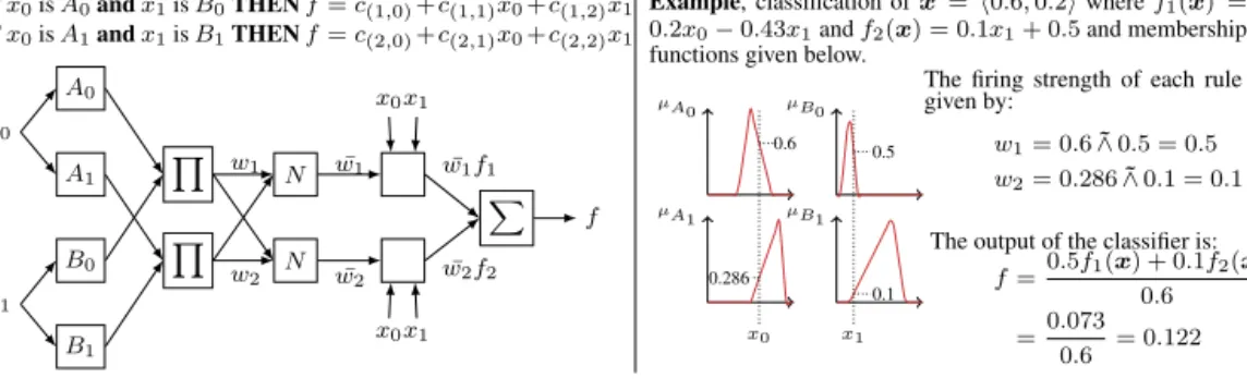
TS-ANFIS implements classification as inference in a system of fuzzy IF-THEN rules. Each rule is composed of an antecedent and consequence part. The antecedent is composed of a fuzzy set for each input variable of the classifier and the consequence is a polynomial mapping the input variables to the output domain. A two rule example classifier is shown in Figure 1for two input variablesx0 andx1 where the 4 Possibility measures are special cases of plausibility functions in Dempster-Shafer theory[2], a general-ization of Bayesian probability theory
5 Using the duality theorem the inverse order of this join semi-lattice is a meet semi-lattice, where in our case the elements would correspond to measures ofN(x) since Π(x) = 1−N(x).
IFx0isA0andx1isB0THENf=c(1,0)+c(1,1)x0+c(1,2)x1 IFx0isA1andx1isB1THENf=c(2,0)+c(2,1)x0+c(2,2)x1 x0 x1 A0 A1 B0 B1 N N x0x1 x0x1 f w1 w2 ¯ w1 ¯ w2 ¯ w1f1 ¯ w2f2
Example, classification ofx =0.6,0.2 wheref1(x) = 0.2x0−0.43x1andf2(x) = 0.1x1+ 0.5and membership functions given below.
μA0 μB0 μA1 μB1 x0 0.6 0.286 x1 0.5 0.1
The firing strength of each rule is given by:
w1= 0.6˜∧0.5 = 0.5
w2= 0.286∧˜0.1 = 0.1 The output of the classifier is:
f=0.5f1(x) + 0.1f2(x) 0.6 =0.073
0.6 = 0.122
Fig. 1. First-order Takagi-Sugeno ANFIS with two rules and two variables
fuzzy sets in the antecedent part is calledA0 (A1) andB0 (B1) for the first (second)
rule respectively and similarly the coefficients of the polynomial of the consequence part is denoted c1,i (c2,i). The classifier is composed of five layers. The first three layers look up the fuzzy membership degrees of the input vector and compute the normalized fuzzy conjunction of this collection, producing the normalized firing strengthof the rule, i.e. the fuzzy membership or weight of the rule. In the example the fuzzy membership of the input vector isμA0(x0) = 0.6 andμB0(x1) = 0.5. The
fuzzy conjuncture of the min-max fuzzy-logic evaluates tow1=min(0.5,0.6) = 0.5,
similarly w2 = 0.1, and hence the normalized weight is ¯w1 = w1w+w1 2 = 0.50.6. The
next layer weight the consequent outputfi(x) with the normalized firing strength. The final layer sums each weighted rule classification. Returning to the example we get f1(x) = 0.034 andf2(x) = 0.56 hence the output of the classifier is 0.50.60.034 +
0.1
0.60.56 = 0.122. Since the consequent part is a polynomial and the classification can
be improved online using algorithms for statistical regression/adaptive filtering, e.g. Least Mean Square (LMS). We use TS-ANFIS and LMS when we can guarantee convergence for the dynamical analysis in Section3.2.
3
Fuzzy set abstraction
Program analyses reason about the dynamics of the individuals of the analysis (e.g. memory stores, redundant expressions) with respect to a set of properties. The 3-valued logic analysis of Sagiv et al.[10] uses logical predicates to state when individuals possess a property, and logical formulas to model how statements up-date predicates. Their framework relies on first-order 3-valued Kleene logic with transitive closure and bi-lattice theory [4], where inference values are ordered both according to a information order and a truth order. The framework crucially en-ables summarizing predicates over a potentially infinite number of individuals and interpretations in a concrete semantics to a finite, tractable program analysis.
Our interest in increasing the precision of analyses and incorporating dynamic information leads us to consider analyses where individuals can possess properties to a certain degree. To this end we use a family of fuzzy logics.
One of the simplest forms of fuzzy logics is Kleene’s 3-valued logic as used by Sagiv et al.[10] which we get by restricting the min-max fuzzy logic to three
values. We will therefore use their program analysis framework as a basis for our own fuzzy set abstraction which is described in Section 3.1. Although analyzes in our framework are decidable and sound the resulting abstract description could, in the worst-case, be very large. Therefore we also consider cases where the resulting description is kept to a minimum. Analyses in this approximation yield a single interpretation representing the maximum interpretation.
3.1 Static analysis
Similar to Sagiv et al.[10]we start with a given set of predicates, avocabulary,P =
{p1, ..., pn}. A program statement, which defines the new state for each property of
each individual, is modeled as apredicate transformer, i.e. a logical formula over P that transforms a predicate into a new predicate.
Definition 3.1 LetPbe a vocabulary. Aprogram statementis a set of predicate transformers, one for each predicatep∈ P. A predicate transformer is described by a logical formula φ from the grammar below. A Flow graph is a edge-labeled connected graphG=V ∪ {vstart}, E, Cwherevstartis the unique start node with
zero in-degree, nodes v∈V are program statements, edges e ∈E⊂V ×V denote control transfer between two vertices and C maps an edge to its control transfer condition.
φ::= ⊥ | |p(v1, ..., vk)| ¬φ | φ∧φ | φ∨φ| ∀v:φ| ∃v:φ | T Cv1, v2:φ
The concrete semantics defines the set of possible 2-valued logical structures that satisfy a predicate transformer. The semantics of a formula is defined in the standard way for 2-valued logics with transitive closure.
Definition 3.2 [Sagiv et al.[10], def. 3.2] LetUS be a universe of individuals and
P =P1∪ P2...∪ Pk a set of unary, binary,..., k-ary predicates.
• 2-valued interpretation is a structureS=US, iSwhereiS(p∗) is a map from US∗ to a truth value (i.e., 0 or 1), p∗ ∈ P∗. The set of 2-valued interpretations is denoted 2-ST RUCT[P].
• Anassignment ZS is a mapping from variables to individuals, i.e. Z :V → US. The assignment iscompleteif Z is total.
• The free variables of a formulaφis defined in the standard way. If free(φ) =∅ we sayφ is aclosed formula.
• 2-valued meaning[[φ]]S2(Z) of a closed formulaφ and a complete assignment Z yields a truth value and defined inductively in Figure 2(left)
• S andZ satisfyφ if [[φ]]S2(Z) = 1. We denote this byS, Z|=φ, or S|=φ if φ is satisfied for allZ.
A statement updates each property (of each individual) according to a prede-fined transfer function. The semantics of a statement should hence generate new predicates, defined in terms of the predicates of its predecessors.
[[⊥]]S2(Z) = 0 [[⊥]]S[0,1]q(Z) = 0.0 [[]]S2(Z) = 1 [[]]S[0,1]q(Z) = 1.0 [[¬φ]]S2(Z) = 1−[[φ]]S2(Z) [[¬φ]]S[0,1]q(Z) =¬˜ [[φ]]S [0,1]q(Z) [[p(v1, ..., vk) ]]S2(Z) =iS(p)Z(v1), ..., Z(vk) [[p(v1, ..., vk) ]]S[0,1]q(Z) =iS(p)Z(v1), ..., Z(vk) [[φ1∧φ2]]S2(Z) = min [[φ1]]S2(Z),[[φ2]]S2(Z) [[φ1∧φ2]]S[0,1]q(Z) =∧˜[[φ1]]S[0,1]q(Z),[[φ2]]S[0,1]q(Z) [[φ1∨φ2]]S2(Z) = max [[φ1]]S2(Z),[[φ2]]S2(Z) [[φ1∨φ2]]S[0,1]q(Z) =∨˜[[φ1]]S[0,1]q(Z),[[φ2]]S[0,1]q(Z) [[∀v:φ]]S2(Z) = minu∈US[[φ]]S2Z[v→u] [[∀v:φ]]S[0,1]q(Z) = ∧˜ u∈US [[φ]]S [0,1]q Z[v →u] [[∃v:φ]]S2(Z) = maxu∈US[[φ]]S2Z[v→u] [[∃v:φ]]S[0,1]q(Z) = ∨˜ u∈US [[φ]]S [0,1]q Z[v →u] [[T C v1, v2:φ]]S2(Z) = [[T C v1, v2:φ]]S[0,1]q(Z) = max u[0,n]∈U Z(v1) =u0 Z(v2) =un n−1 min i=0[[φ]] S 2 ⎛ ⎝Z v1→ui v2→ui+1 ⎞ ⎠ ∨˜ u[0,n]∈U Z(v1) =u0 Z(v2) =un n−1 ˜ ∧ i=0[[φ]] S [0,1]q ⎛ ⎝Z v1→ui v2→ui+1 ⎞ ⎠
Fig. 2. Definition of the semantics of classical first-order logic with transitive closure (left) and first-order fuzzy logic with transitive closure over the congruence domain [0,1]q(right)
of unary, binary,... k-ary predicates, let φwp be the formula with free variables v1, ..., vx which updates predicatepat statement w. Given a structure S we define
the semantics ofS after w as
[[st(w)]]2(S) =US,kx=1λp∈ Pxλu1, ..., λux.[[φwp]]S2([v1→u1, ..., vx→ux])
. The 2-valued semantics define the (possibly infinite) set of logical structures that a node may see on entry. The collecting semantics is later defined as the least fixed-point of the 2-valued semantics.
Definition 3.4 Let V S map v ∈ V to a set of 2-valued logical structures. The 2-valued semantics of a flow graph G=V, E, Cis given by
[[G]]2(V S) =λv. ⎧ ⎪ ⎪ ⎨ ⎪ ⎪ ⎩ V S(vstart) v=vstart w→v∈E [[st(w)]]2(S)|S ∈V S(w) andS|=C(w, v) otherwise The natural order on [0,1] has infinite height, hence includes infinite chains. Fix-point iteration in such a domain may not terminate. Widening operators solve this problem by traversing the domain in a finite number of steps, e.g. by a sequence of
jumps in the domain followed by the top/bottom element. However, its very hard to control the degree of over-approximation introduced by a widening operator. Rather than introducing a widening operator we let our fuzzy abstraction use a finite congruence domain of the unit interval. To trade expressiveness for tractability, or vice versa, we define the abstract semantics over a family of congruence domains over [0,1]: the q domains, whereq ∈N− {0}. The domains are linearly ordered
such that a truth valuetinqis split to two truth values (not including 0.5) inq+1.
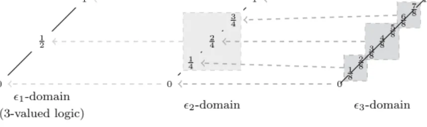
We illustrate the congruence relation in Figure 3 for the 1 (i.e., 3-valued Kleene
logic used by Sagiv et al.[10]),2 and3. The values in the light gray box of2 (i.e.
1/4, 1/2 and 3/4) are therefor mapped to 1/2 in1and similarly the dark gray boxes
1 1 2 0 1-domain (3-valued logic) 1 3 4 2 4 1 4 0 2-domain 1 7 8 6 8 5 8 4 8 3 8 2 8 1 8 0 3-domain
Fig. 3. Equivalence partitioning of the1,2and3graded truth orders
relation is consistent with the information order introduced in Section 2,i.e., when interpreting a q+1 value in aq domain the value is never moreinformative.
Definition 3.5 The q equivalence class of x ∈[0,1], denoted [x]q, is defined by rounding x to the closest multiple of 21q towards 12. The set of all q equivalence
classes is [0,1]q={21qx|x∈N2q}whereN2q =
x|x∈N∧0≤x≤2q.
The abstract semantics overqis defined in terms of the fuzzy logics from Section2.
The definition uses concepts such as interpretation and assignment which is similar to that of the concrete semantics but wheretruth value is now an element of [0,1]q
rather than{0,1}.
Definition 3.6 [Sagiv et al.[10], def. 4.2] The [0,1]q-valued interpretation and
assignment is analogous to the concrete semantics.
• Given a Fuzzy logic ∧˜,∨˜,˜¬ the fuzzy q meaning [[φ]]S[0,1]q(Z) of a closed formula φ and a complete assignment Z yields a truth value in [0,1]q and defined inductively in Figure2(right)
• The definition of the semantics of a statement (i.e., [[st(w)]][0,1]q) is analogous to the concrete case in Definition 3.3 but the formulas are interpreted in a given fuzzy logic.
• SandZpotentially satisfyφif [[φ]]S[0,1]q(Z)>0. We denote this byS, Z|=[0,1]q
φ, or S|=[0,1]q φif φ is satisfied for allZ.
Embeddings was introduced by Sagiv et al.[10]to relate 2-valued and 3-valued inter-pretations. Informally they relate logical structures that conform to an information order. The embeddings cluster individuals and decide the value of their properties in terms of the corresponding values of the members of the cluster. Importantly, the class of embeddings that minimize information loss is termedtight and are used to define the abstract semantics of a flow-graph. Note that although we choose to cluster individuals here it is also possible to cluster predicates[7] as in a predicate abstraction.
Definition 3.7 LetS=US, iSandS =US, iSbe two [0,1]q-interpretations.
satisfies below relation. The embedding istightif the relation holds for equality. ∀x∈[1, k],∀p∈ Px:iS(p)(u1, ..., ux) (u1, ..., ux)∈(US)x f(ui) =ui,1≤i≤x iS(p)(u 1, ..., ux)
The abstract semantics need to preserve information loss to be conservative (i.e. should not spuriously introduce more precise results). For this reason our abstract semantics is monotonically increasing with respect to an information order.
Lemma 3.8 (Sagiv et al.[10], Lemma 4.4) LetS =
US, iSandS=US
, iS
be two structures whereS =S and let f :US →US be a -embedding. Then for every complete assignment Z, all k-arity p ∈ Pk: iS iS ⇒ [[φ]]S[0,1]q [[φ]]S[0,1] q
where iS iS is the point-wise extension of .
Intuitively, given a finite number of individuals (predicates) we should be able to cluster (even an infinite number of) predicates (individuals) into a finite number of clusters such that all predicates (individuals) in a cluster are equivalent with respect to the individuals (predicates). We refer to this special embedding as normaliza-tion6. More specifically the number of clusters from the normalizer is bounded by
|US
| ≤(1 + 2q)
k
i=1|Pi|i in a [0,1]q domain.
Definition 3.9 Let P = P1∪...∪ Pk be the sets of unary (P1), ..., k-ary (Pk) predicates. Two individuals ui, ui ∈ US, ui = uj are equivalent if all predicates evaluate to the same values for ui and uj, i.e. if ∀p ∈ P1 : p(ui) = p(uj) and
∀p∈ P2, u ∈US : [p(u
i, u) =p(uj, u)]∧[p(u, ui) =p(u, uj)] and analogously for allPi,3≤ i≤ k. The normalizer fNorm is a -embedding that generates a new logical structure UˆS,ˆiS that maps equivalent individuals from US to the same individual in ˆUS.
Example 3.10 Let S = {u1, u2, u3, u4, u5, u6}, iS
be as in left most table be-low. Hereu2, u4 andu6 are equivalent w.r.t all predicates (i.e.,p, q andr). Shown
in the right most table below is the resulting structure when applying the nor-malizer, where equivalent individuals are represented by a new individual u246.
Individual Unary predicate
p q r u1 1 0 1 u2 1 1 0 u3 0 1 0 u4 1 1 0 u5 1 1 1 u6 1 1 0
Individual Unary predicate
p q r
u1 1 0 1 u246 1 1 0 u3 0 1 0 u5 1 1 1
Using normalization we can hence produce a logical structure with a finite num-ber of individuals, and by extension, bound the numnum-ber of logical structures. We
also consider the extreme case of normalization, when the set of logical structures is a singleton. To accommodate both cases we parameterize the abstract semantics on a functionFn, thecollector function that takesnsets (representing the results from nincoming edges) of logical structures and produce a single set of logical structures. We consider the following F∗ and∗ combinations:
(i) (n≥1) Thebounded union semantics with∪ andF∪n(S) =
n
i=1Si
. (ii) (n= 1) Themaximum semantics with and
Fn (S) = USˆ ,kx=1{λu1, ..., λux. n y=1iSy(p) [v1→u1, ..., vx →ux] |p∈ Px}.
We introduce an abstract semantics as the fixed-point, with respect to set-inclusion (whennis bounded) or the information order (whenn= 1) from Section2.2, of the equation system below and show that it over-approximates the collecting semantics.
Definition 3.11 Let F∗n be a collector function and f be a tight ∗-embedding andV Smapv∈V to a set of bounded [0,1]q-valued logical structures. The [0,1]q -valued semantics of a flow graphG=V, E, Cis given by
[[G]][0,1]q(V S) =λv. ⎧ ⎪ ⎪ ⎪ ⎪ ⎪ ⎪ ⎨ ⎪ ⎪ ⎪ ⎪ ⎪ ⎪ ⎩ F1 ∗V S(vstart) v=vstart Fn ∗ ⎛ ⎜ ⎜ ⎝ ⎧ ⎪ ⎨ ⎪ ⎩f [[st(w)]][0,1]q(S) S∈V S(w) and S|=[0,1]q C(w, v) ⎫ ⎪ ⎬ ⎪ ⎭ w→v∈E ⎞ ⎟ ⎟ ⎠otherwise Computing the fixed-point proceeds by iteratively applying a monotonic increas-ing transfer function and terminates in bounded time because the set of possible logical structures is bounded. The result of the analysis is sound as per Theorem
3.12. Note that the result of a fuzzy set abstraction usingFn is the most accurate maximum logical structure a q domain can provide, i.e. within a factor 21q of the
true value.
Theorem 3.12 For a flow graph G=V, E, C and initial assumptions Sentry =
{S0, ..., Sn} ⊂[0,1]q-ST RUCT[P], n∈N the collecting semantics of the flow graph is denoted C and is defined using the 2-valued semantics:
C=lfp⊆[[G]]2({vstart→Sentry} ∪ {v→ ∅|v∈V-{vstart})
The abstract semantics with the bounded union- and the maximum collector func-tions is similarly defined using [0,1]q-valued semantics:
AF∪ =lfpF⊆∪[[G]][0,1]q({vstart→Sentry} ∪ {v→ ∅|v∈V-{vstart}) AF =lfpF[[G]][0,1]q({vstart→Fn(Sentry)} ∪ {v→ 1 2|v∈V-{vstart}) where 1 2 = US, k x=1 p∈Px {λu1, ..., ux.iS(p) [v1→u1, ..., vx→ux] = 0.5}
The corresponding concretization functions are given by γF∪ and γF where [S]1 de-notes the interpretation of structureSin 3-valued logic, i.e. the point-wise extension
of Definition 3.5. γF∪(S) ={S#∈2-ST RUCT[P]|S# [S]1} γF(U, i) = U, i# ∈[0,1]q-ST RUCT[P]| ∀x∈[1, k], p∈ Px, u1, ..., ux∈U : i(p)[v1→u1, ..., vx→ux] −i#(p)[v 1→u1, ..., vx→ux]≤ 1 2q !
With the above definitions in place we can state or main theorem: The concrete semantics is approximated by the composition of the abstract semantics and the concretization function: ∀v: ⎧ ⎪ ⎨ ⎪ ⎩ C(v)⊆ s∈AF∪(v) γF∪(s) C(v)⊆γF AF(v) 3.2 Dynamical analysis
We next explore an dynamical analysis which starts from the results of the static analysis with an q domain and improves the accuracy by specializing the analysis
result given a sequence of dynamical assignments of a property. The aim is to improve completeness, possibly sacrificing soundness, and compute a new fuzzy set with increased classification accuracy. The resulting fuzzy set is described implicitly by an TS-ANFIS. We consider improving the accuracy with respect to the least square error between the example(s) and the analysis results.
Our dynamical analysis instantiate an TS-ANFIS and use gradient descent (GD) to improve classification online. GD is similar to Newton’s method and so we use results from Newtonian program analysis[3]in formalizing our dynamic analysis.
Esparza et al. [3] showed that polynomials f(x) = "iciφi(x) = "ici#jx ai,j i,j
overω-continuous (commutative) semirings admit points due to Kleene’s fixed-point theorem. Since membership of a fuzzy set is an element of the unit interval [0,1] we use the special case of polynomials over the real semiringR∪ {∞},+,·,0,1. We let ∂x∂f
i denote the (partial) derivative of f with respect to the variable xi, ∇f = "i ∂x∂f
iei denote its gradient and Dfν(x) = ∇f(ν)·x the differential of a
polynomial f. We stress that our polynomials are evaluated on a congruence do-main of the real semiring, i.e. an q domain. In this article we consider the case
when the resulting set of logical structures from the static analysis is a singleton, i.e., the result was computed using the maximum abstract semantics above7.
The logical structure, i.e. S= U, i, can be considered a set of classifiers, one for eachk-ary predicatep∈i, where the variables are assigned an individual (fromU) as input value. Givenp we create a two rule TS-ANFIS where the variables x[1,k] are real-valued encodings of the individuals, e.g. the encodingui→i.
7 It is possible to extend our scheme to an arbitraryn∈Nby building an TS-ANFIS with 2nrules. But
this obviously comes at a high cost and for lack of a better scheme we postpone formalization to future work
Newton’s method f+ Newton(νi)=lfp Df νi(f(νi)−ν) f− Newton(νi)=gfp Df νi(ν−f(νi)) GD onx, y f+ GD(νi)=μ·lfp ∇(νiφi(x)−y)2 f− GD(νi)=μ·gfp ∇(y−νiφi(x))2 Table 1
Newton/GD fixed-point equation
• (Rule 1) p is the fuzzy set in the premise part and f(x1, ..., xk) = 1 is the
consequent polynomial.
• (Rule 2) ¬˜p is the fuzzy set in the premise part and f(x1, ..., xk) = 0 is the
consequent polynomial.
The output of the initial TS-ANFIS is hence equal to the predicate p. Our dynam-ical analysis is iteratively given an example assignment x and the corresponding
actual fuzzy membership y. It computes a new fixed-point when x is the input producing the expected fuzzy membership and updates the consequent polynomials f(x) based on the error. The algorithm used for rule 1 minimizes the polynomial coefficient corresponding to the constant (which were initialized to 1) and maximizes the remaining coefficients (which was initialized to 0). The polynomial for rule 2 remains constant. Table 1 shows the fixed-point equations. Note that elements of a semiring do not in general have an additive inverse, hence subtraction may seem erroneous. But as noted by Esparza et al. [3]for the particular case when the func-tion is a polynomial in a semi-ring the difference is always positive, a consequence of a generalized form of Taylors theorem. For a commutative semiring the accuracy increases exponentially with each iteration[6]. The number of elements in a q do-main is 2q. Hence each iteration of our dynamical analysis produce the fixed-point in theq+1domain.
Lemma3.13shows that the fixed-point systems admit a solution. As all ascend-ing/descending chains are finite in an q domain the sequence will, assuming x is
monotonically decreasing/increasing, converge to a new consequent polynomial.
Lemma 3.13 Letf(x) be a polynomial. Then the ascending/descending sequence
νi
i∈N is increasing/decreasing monotonically and converges to unique
least/great-est fixed-point:
• 0≤νi≤f+(νi)≤νi+1≤sup≤ j∈Nνj • inf≤j∈Nνj ≤νi+1≤f−(νi)≤νi≤1
The fixed-point equations admit a recursive closed-form that we state in Lemma
3.14. Our results show that we can guarantee validity in the real semiring by imposing constraints on the inputs rather than resorting to a non-negative version of the GD algorithm[1].
Lemma 3.14 Given ax, y and a polynomialf(x)lete(k) =f(x)−y forf+and
e(k) =y−f(x) forf−. We can compute f∗ using ck+1i,j =cki,j+ 2μei(k)φ(x).
Finally, we show in Theorem 3.15 that our dynamical analysis indeed improve the analysis results for a set of examples.
be the analysis result with the Fn abstract semantics and x, y1≤i≤N a sequence of examples such that ∀j : xji+1 ≤ xji and yi+1 ≤ yi. Then each iteration i of the GD algorithm, applied to the example x, yi, updates the polynomials such that the coefficients are non-negative and in the limit converge to a polynomial that minimize the least square error to the set of examples.
4
Conclusion
We have introduced the Fuzzy Set Abstraction which enables stating properties about programs which are true or false to a certain degree. This opens up new possibilities for speculative optimizations which can now use information about which values, branches, etc. are more likely than others.
We have also shown how to perform hybrid analysis by refining the result of a static analysis online. This has been done using TS-ANFIS, an adaptive fuzzy inference system from control theory. This result paves the way for importing other results from the rich literature of fuzzy control theory.
References
[1] Chen, J., C. Richard, J. C. M. Bermudez and P. Honeine,Nonnegative least-mean-square algorithm, IEEE Transactions on Signal Processing59(2011), pp. 5225–5235.
[2] Dubois, D., H. Prade and H. Prade, “Fundamentals of Fuzzy Sets,” The Handbooks of Fuzzy Sets, Springer US, 2000.
[3] Esparza, J., S. Kiefer and M. Luttenberger,Newtonian program analysis, J. ACM57(2010), pp. 33:1– 33:47.
[4] Ginsberg, M., Multivalued logics: A uniform approach to inference in artificial intelligence, Computational Intelligence4(1988), pp. 265–316.
[5] Lidman, J. and J. Svenningsson, Bridging static and dynamic program analysis using fuzzy logic, Quantitative Aspects of Programming Languages and Systems (QAPL) (2017).
[6] Luttenberger, M. and M. Schlund, “Convergence of Newton’s Method over Commutative Semirings,” Springer Berlin Heidelberg, Berlin, Heidelberg, 2013 pp. 407–418.
[7] Manevich, R., E. Yahav, G. Ramalingam and M. Sagiv, “Predicate Abstraction and Canonical Abstraction for Singly-Linked Lists,” Springer Berlin Heidelberg, Berlin, Heidelberg, 2005 pp. 181– 198.
[8] Mock, M., M. Das, C. Chambers and S. J. Eggers,Dynamic points-to sets: A comparison with static analyses and potential applications in program understanding and optimization, in:Proceedings of the 2001 ACM SIGPLAN-SIGSOFT Workshop on Program Analysis for Software Tools and Engineering, PASTE ’01 (2001), pp. 66–72.
[9] Ribeiro, C. and M. Cintra,Quantifying uncertainty in points-to relations, in:Languages and Compilers for Parallel Computing, Lecture Notes in Computer Science 4382, Springer Berlin Heidelberg, 2007 pp. 190–204.
[10] Sagiv, M., T. Reps and R. Wilhelm,Parametric shape analysis via 3-valued logic, ACM Trans. Program. Lang. Syst.24(2002), pp. 217–298.
A
Omitted proofs
Proof. of Theorem 3.12. We first consider the case when using the F∪ function, Note that γ(S) creates the set of all 2-valued logical structures that are ∪ S,
quantized to the1domain (i.e., the 3-valued domain in Sagiv et al.[10]by Definition
3.5). Since generatingS(i.e., the fixed-point iteration) was done conservatively by Theorem3.8we can re-use the argument from Sagiv et al.[10]Theorem 4.9 (i.e., that an embedding is extensive w.r.t. to the information order: [[φ]]S2(Z)[[φ]]S3(f◦Z)), Theorem 6.1 (i.e., that we are conservative w.r.t. a branch condition and program statement) and Theorem 6.2 (i.e.,∀v:C(v)⊆s∈A(v)γ(s)).
We next consider the case when using the F function. Note that, as per Knaster-Tarskis fixed-point theorem the abstract semantics is well-defined. We ar-gue that the result is a conservative approximation (i.e., ∀v:C(v)⊆γF
AF(v)
) based on proof by contradiction on the existence of a fixed-point for the collectors Fn
: Assume an fixed-point S∞ has been reached then S∞(v), v∈V is the unique
maximal element in q. γF(S∞(v)) is the set of [0,1]q logical structures where the
predicates are within 21q from S∞(v). If S∞ is not a conservative approximation
then there exists an elementS∗∈γF(S∞(v)) that is further away fromγF(S∞(v))
than 21q which contradict that S∞ is the unique fixed-point. 2 Proof. of3.13This is a special case of Theorem 3.10 in Esparza et al.[3]with the
(non-negative) real semiring. 2
Proof. of3.14. As the fixed-point iteration is performed over a totally ordered set (the least square error) the minimal/maximal and infimum/supremum element co-incide. We consider finding the coefficients ci of a polynomialf(x) ="iciφi(x) =
"
ici#jx ai,j
i,j that minimize the least square error, e(x)2 =
f(x)−y2 at a par-ticular x, y. Sincee(x)2 is convex we know that globally minimal solution occur where gradient is zero:
∂f(x)−y2 ∂c = 2 f(x)−y· ∂ " iciφi(x)−y ∂c = 2f(x)−yφ(x) = 2e(x)φ(x)
Hence maxcif(x)−y2 = 2e(x)φ(x) and since the expression only depends on
variables in the current iteration the sequence of updates is given by ci+1 = ci+ 2μe(x)φ(x). Similary minciy−f(x)2 = −2e(x)φ(x) and hence ci+1 = ci −
−2e(x)φ(x)=ci+ 2e(x)φ(x). 2
Proof. of 3.15. Lemma 3.14 shows that each iteration finds the coefficients that minimize the least square error. Toghether with monotonicity ofx &yand Lemma
![Fig. 2. Definition of the semantics of classical first-order logic with transitive closure (left) and first-order fuzzy logic with transitive closure over the congruence domain [0, 1] q (right)](https://thumb-us.123doks.com/thumbv2/123dok_us/610107.2573103/7.727.77.621.96.370/definition-semantics-classical-transitive-closure-transitive-closure-congruence.webp)