A two-stage stochastic integer programming approach

DOCUMENTOS DE TRABAJO

BILTOKI

Facultad de Ciencias Econ ´omicas. Avda. Lehendakari Aguirre, 83

48015 BILBAO.

D.T. 2005.01

A two-stage stochastic integer programming approach .

Documento de Trabajo BILTOKI DT2005.01

Editado por el Departamento de Econom´ıa Aplicada III (Econometr´ıa y Estad´ıstica)

de la Universidad del Pa´ıs Vasco.

Dep´osito Legal No.: BI-292-05

ISSN: 1134-8984

A two-stage stochastic integer programming approach

as a mixture of Branch-and-Fix Coordination and

Benders Decomposition schemes

L.F. Escudero1, A. Gar´ın∗2, M. Merino∗3 and G. P´erez∗4

1_{Centro de Investigaci´on Operativa}

Universidad Miguel Hern´andez, Elche (Alicante), Spain e-mail: [email protected]

2_{Dpto. de Econom´ıa Aplicada III}

Universidad del Pa´ıs Vasco, Bilbao (Vizcaya), Spain e-mail: [email protected]

3_{Dpto. de Matem´atica Aplicada, Estad´ıstica e Investigaci´on Operativa}

Universidad del Pa´ıs Vasco, Bilbao (Vizcaya), Spain e-mail: [email protected]

4_{Dpto. de Matem´atica Aplicada, Estad´ıstica e Investigaci´on Operativa}

Universidad del Pa´ıs Vasco, Leioa (Vizcaya), Spain e-mail: [email protected]

Abstract

We present an algorithmic approach for solving two-stage stochastic mixed 0-1 prob-lems. The first stage constraints of the Deterministic Equivalent Model have 0–1 vari-ables and continuous varivari-ables. The approach uses theTwin Node Family(TNF) concept within the algorithmic framework so-called Branch-and-Fix Coordination for satisfying thenonanticipativityconstraints, jointly with a Benders Decomposition scheme for solv-ing a given LP model at each TNFinteger set. As an illustrative case, the structuring of a portfolio of Mortgage-Backed Securities under uncertainty in the interest rate path along a given time horizon is used. Some computational experience is reported.

Keywords: Two-stage integer programming, Benders decomposition, nonanticipativ-ity constraints, splitting variables, twin node family, branch-and-fix coordination, MBS portfolio structuring.

* This research has been partially support by the grant Grupo consolidado de alto rendimiento 9/UPV 00038.321-13631/2001 from UPV, the project MEC2001-0636 from the DGCIT, the Researchers’ Education grant program 2000 from Gobierno Vasco, and the grant GRUPOS79/04 from the Generalitat Valenciana, Spain.

Introduction

Very frequently, mainly in problems with a given time horizon to exploit, some coefficients in the objective function and the right–hand–side (rhs, for short) vector and in, a lesser extend, the constraint matrix are not known with certainty when the decisions are to be made, but some information is available. This circumstance allows to use Stochastic Integer Programming (SIP) for solving (mixed) 0–1 programs under uncertainty. It has a broad application field, mainly, in production planning (Mirhassani et al. (2000), Klein Haneveld & van der Vlerk (2001), Ahmed et al. (2003), Alonso-Ayuso et al. (2003b,c, 2004, 2005) and Lulli & Sen (2004)), energy generation planning (Takriti & Birge (2000), Gr¨owe-Kuska et al. (2001), Hemmecke & Schultz (2001), Klein Haneveld & van der Vlerk (2001), Nowak et al. (2002), N¨urnberg & R¨omisch (2002) and Triki et al. (2005)) and finance (Cohen & Thore (1970), Crane (1971), Mulvey & Vladimirou (1992), Zenios (1995a), Cari˜no & Ziemba (1998), Ziemba & Mulvey (1998), Fleten et al. (2002), Kusy & Ziemba (2002)), among others (Uryasev & Pardalos (2001), Laporte & Louveaux (2002), Maatan et al. (2002) and Wallace & Ziemba (2005)) and, specially, see the books Jarrow et al. (1995), Zenios (1995b), Ziemba & Mulvey (1998) and Scherer (2003) devoted to financial management. See also Schultz (2003). The main focus and contribution of the paper is on the design and computational as-sessment of a Branch-and-Fix Coordination (BFC) scheme for obtaining the optimal mixed 0–1 solution to the two-stage stochastic program, where the parameters’ uncertainty is rep-resented by a set of scenarios. An important feature of our approach with respect to some other approaches for two-stage SIPis that it addresses the problemwhere 0–1 variables and continuous variables have nonzero elements in the first stage constraints. The difficulty in the algorithmic approach is very much increased by having the continuous variables in the first stage constraints. The special structure of the Deterministic Equivalent Model (DEM) is exploited. The relaxation of thenonanticipativity constraints of the first stage variables allows for the independent solution of the so–called scenario cluster-related problems. The constraints related to the 0–1 variables are satisfied by using a scheme that is based on the Twin Node Family(TNF) concept introduced in Alonso-Ayuso et al. (2003a,c). The scheme is specifically designed for coordinating the node branching selection and pruning and the 0–1 variable branching selection and fixing at each Branch-and-Fix(BF) tree.

Additionally, the proposed approach considers thecompactrepresentation of theDEMat eachTNFinteger set. By fixing those variables to the nodes’ values, theDEMhas only con-tinuous variables. By exploiting the remaining model’s structure, a Benders Decomposition allows thenonanticipativity constraints on the first stage continuous variables to be satisfied and, so, obtaining theLPoptimal solution for the givenTNFinteger set. The conditions for pruning aTNFare stated.

Given a time horizon, a set of available securities and an available budget for investment, theMortgage-Backed Securities Portfolio Structuring Problem(MBSPSP) is concerned with determining the subset of securities that will be included in the portfolio as well as determining the fraction of the face value to consider for each security, under uncertainty in the interest rate path along the time horizon. The problem of concern can be viewed as the problem considered in Escudero (1995), see also Zenios (1993), but forcing an upper bound on the number of securities to include in the portfolio and requiring a conditional minimum on the face value for each security, among other types of constraints for structuring the portfolio.

The problem can be treated as a two-stage stochastic mixed 0–1 model. The first stage constraints in the problemhave the 0–1 variables for determining the securities to include in the portfolio, and the continuous variables for determining the fraction of the related face value to consider. The second stage constraints have only continuous variables under each scenario, for determining the net available cash at the so-called dedicated time periods and for representing certain types of mismatchings related to durations and present values. So, theMBSPSP can be considered as an illustrative case for the computational assessment of our approach for two-stage SIPproblem solving. Some computational experience is reported to compare the quality of the solution obtained by our approach and the optimization of the average scenario problem. A comparison is also performed with solving the DEMby a plain use of a state-of-the-art optimization engine.

The remainder of the paper is organized as follows. Section 1 states theMBSPSP. Section 2 presents the m ixed 0-1 DEM. Section 3 presents the TNF based BFC algorithmic frame-work for problemsolving. Section 4 presents an illustrative case. Section 5 reports on the computational results. Section 6 concludes.

1

Problem statement

Let a security be defined as an asset that entitles the holder to a return along a time horizon. In our case, the asset is a financial right included by a principal and a yield backed by a mortgage (so, it is calledMortgage-Backed Security, for shortMBS), whose principal can be prepaid and even delayed. So, each security (e.g., a loan) to consider for being included in the portfolio should have the following features: principal’s amortization structure up to its maturity period; (usually adjustable) yield to be paid over time; partial or full potential prepayment, such that the prepayment of a security will affect its duration and the cashflow to generate; potential delay of the principal’s amortization; and type of risk measured by the interest rate weighting factor, the so-calledOption Adjusted Spread (OAS).

The OAS is used to weight the discount rate for obtaining the present value of a given security. It can be interpreted as the implied risk penalty for a particular security, see Hayre & Lauterbach (1991) and Ben-Dov et al. (1992), among others. Note: The value 0 (resp., 1) means a neutral factor for anadditive (resp.,multiplicative) scheme, see below.

TheMBSsecuritization consists of structuring a portfolio froma set of available securities. The problemof concern consists of the MBS securitization under the uncertainty in the interest rate path along a given time horizon, which implies uncertainty in the securities’ yield, prepayment and payment delay. As we said above, the uncertainty is represented by a set of scenarios. One characteristic of our problemis the need to resort to an integer formulation (rather than using only continuous variables). That need is motivated by the problem’s requirements related to the maximum number of securities to include in the portfolio, the MBS face value conditional minimum, the exclusivity and implicative constraints in the portfolio, etc.

There are three important issues that have not been considered in the paper, namely, the recursive contingent claimoption (Dunn & McConnell (1981) and Schwartz & Torous (1989)), the transaction costs on exercising the options, (Stanton (1995) and Longstaff (2004)) and the heterogeneity among mortgage borrowers for determining theMBSs(Deng et al. (2000)).

Although important issues, they are not crucial for assessing the performance of the proposed algorithmic approach for optimizing two-stage SIPproblems.

A feasible structuring of a portfolio requires two types of constraints to be satisfied, namely: (a) first stage constraints that force some types of relationships among the securities, e.g., upper bound on the number of securities to be included in the portfolio, investment budget for the securities’ total face value, equilibriumin the total face value of the different types of securities, exclusivity and implicative relationships among those types, etc.; and (b) second stage constraints for basically analyzing the performance of the securities’ portfolio along the time horizon over the scenarios. Typical constraints are the portfolio’s cashflow balance equation including the cash inflow and outflow due to the liabilities’ satisfaction for each dedicated time period under any scenario, the lower and upper bounds for the net available cash in those periods under any scenario, the requirement that the present value of the portfolio is not smaller than the present value of the liabilities under any scenario, the requirement that the absolute mismatchings of the unit durations and the present values of theMBS in the portfolio and the set of securities where it is taken fromare not greater than given thresholds, etc.

There are different types of goals. Thescenario trackingthrough the minimization of the expected difference between the MBS portfolio’s and liabilities’ duration mismatching and the optimal related mismatching under any scenario is treated in Escudero (1995). However, we consider the minimization of the expected absolute mismatching of the durations of the MBS portfolio and the liabilities over the scenarios. It is another approach for hedging the investment’s return against small changes in the interest rate along the time horizon, for given portfolio management fees and others.

The notation to be used through the paper is as follows. Sets:

I, set of available securities.

T, set of time periods.

Ω, set of scenarios to represent the uncertainty. Deterministic parameters:

b₁, maximum number of securities that are allowed in theMBS portfolio to structure. b₂, right-hand-side vector for the subsystemof constraints for the 0-1 variablesδ_i,i∈ I. A₂, constraint matrix for the subsystem of constraints for the 0-1 variablesδ_i,i∈ I. b₃, available investment’s budget at time period 0 to create theMBS portfolio.

h, investment’s net unit return (including management fees) from the investmentb₃ as a target to reach for each so-called dedicated time period.

α_t, investment’s amortization considered for time periodt, for t∈ T, such that b₃ =

t∈T

ϕ_t, liability to be satisfied at (the end of) dedicated time periodt, for t∈ T. It can be expressed as

ϕ_t=α_t+h

τ∈T:τ≥t

α_τ. (2)

, latest dedicated time period where the cash inflow from the portfolio is committed to satisfy the liabilities, for ∈ T.

σ, σ, unit lower and upper bounds of the investment’s face value that is allowed to be kept in cash at any dedicated time period, respectively.

s_t, s_t, lower and upper bounds of available cash at dedicated time periodt, respectively, fort= 1, . . . , , such that

s_t=σ τ∈T:τ >t α_τ (3) s_t=σ τ∈T:τ >t α_τ. (4)

f_i, principal (face) value of security i, fori∈ I.

x_i, x_i, conditional lower and upper bounds of the principal (face) value out of f_i for security ito be included in theMBS portfolio, respectively, fori∈ I.

t_i, maturity period for securityi(i.e., last period where any payment has been planned). Note: t_i ∈ T,∀i∈ I.

a_it, unit principal’s amortization of security i at (the end of) time period t, for t = 1, . . . , t_i, i∈ I.

A_it, cumulated unit principal’s amortization of security i at time period t, for t = 1, . . . , t_i, i∈ I, such that

A_it=

τ=1,...,t

a_iτ, (5)

so that A_it= 1 for t=t_i.

cξ_i, extra interest rate to charge for each time period with payment delay in securityi, fori∈ I.

o_i, OASassigned to securityi, for 0≤o_i, i∈ I.

τ, maximum number of time periods where a principal’s amortization payment can be delayed for any security. Note: τ ≤ |T | −t_i, i∈ I.

Uncertain and scenario related parameters:

wω_{, weight factor assigned to scenarioω, for ω∈Ω, such that}

ω∈Ωwω = 1.

rω_t, interest rate at time periodtunder scenarioω, for t∈ T, ω∈Ω. The scenarios for the interest rate path along the time horizon can be generated from the binomial lattice approach given in Black et al. (1990) as it is done in Zenios (1993). See other schemes in Frauendorfer & Sch¨urle (1998) and Mulvey & Thorlacius (1998). An application of the so-called contamination technique (Dupacova (1986)) is presented in Dupacova et al. (1998) for the analysis of the influence of additional scenarios to a given sample in

bond portfolio management. The stochastic decomposition method for dealing with two-stage stochastic programs via sampling is described in Higle & Sen (1996). See in Kleywegt et al. (2001) and Ahmed & Shapiro (2002) some approaches for approximating the underlying two-stage stochastic program with integer recourse via sampling, among other approaches for dealing with the size of the scenario set. See in Dupacova et al. (2003) an approach for scenario reduction.

cω_it, unit yield of security i at (the end of) time period t under scenario ω. It is a function of the interest rate rω_t and the own security under scenarioω, fort= 1, . . . , t_i, i∈ I, ω∈Ω. Notice thatrω₁ =r₁, where r₁ is the interest rate at timet= 1.

βω

it, (partial or full) prepayment of the cumulated unit principal’s amortization of

secu-rity i at time periodtunder scenarioω, fort= 1, . . . , t_i, i∈ I, ω∈Ω. It is a function of the security, the age of the security, the month of the year and the interest rate at the given period. The function is usually obtained by statistical means. However, see in Kang & Zenios (1992) some complete prepayment models.

κω_itτ, unit payment delay in τ time periods of the principal’s amortization of security i that is due at time period t under scenario ω, for _τ=1,...,τ κω_itτ ≤ a_it, t= 1, . . . , t_i, τ = 1, . . . , τ , i∈ I, ω ∈Ω. It is a function of the security, the month of the year, the number of delay periods and the interest rate at the given time period.

eω_it, net unit principal amortization of securityiat time periodtplus interest payments due to principal delays. It can be expressed as

eω_it = a_it[1− t−1 j=1 β_ijω −(1 +cω_it) τ τ=1 κω_itτ] + τ:1≤t−τ≤τ

a_iτ[1 + (t−τ)(cω_iτ +cξ_i)]κω_iτ(t−τ)

(6)

γ_itω, unit return fromsecurityiat time periodt under scenario ω, fort= 1, . . . , t_i+τ , i∈ I, ω∈Ω. Under mild assumptions, it can be expressed as

γ_itω =eω_it+β_itωA_it+1+cω_itA_it 1− t−1 j=1 β_ijω . (7)

Γω_i, unit return’s present value of security iunder scenarioω, for i∈ I, ω∈Ω. It can be expressed as Γω_i = t=1,...,ti γ_itω τ=1,...,t (1 +o_i·rω_τ)−1. ₍₈₎ Note that o_i has been used as a multiplicative factor of rω_τ and, then, the zero-value is not allowed. However, it is allowed when the OAS is used as an additive factor, see Zenios (1991). Notice that the greater the risk penalty OASo_i is, the smaller the present value Γ_i is,∀i∈ I.

dω

i, change in the unit present value of the return of security i due to a small change

in the interest rate along the time horizon under scenario ω, for i∈ I, ω∈ Ω. It can be expressed as dω_i =−(1/Γω_i) t=1,...,ti t·γ_itω·o_i τ=1,...,t (1 +o_i·rω_τ)−1. ₍₉₎

Note: |dω_i| is the so-called modified Macaulay duration for a flat interest rate along a time horizon.

Φω, present value of the liabilities under scenario ω, forω ∈Ω. It can be expressed as Φω=

t∈T

ϕ_t

τ=1,...,t

(1 +rω_τ)−1. ₍₁₀₎

dω, change in the unit present value of the liabilities due to a small change in the interest rate along the time horizon under scenario ω, for ω ∈Ω. It can be expressed as dω =−(1/Φω) t∈T t·ϕ_t τ=1,...,t (1 +r_τω)−1. ₍₁₁₎

Additional deterministic parameters:

z, upper bound on the absolute difference between the unit duration of theMBS port-folio to structure and the unit duration of the available set of securities I.

v, upper bound on the absolute difference between the unit present value of the MBS portfolio to structure and the unit present value of the available set of securities I. Note. The parameters z and v allow some slackness in the representation of the MBS portfolio with respect to the available set of securities.

Structuring variables. They are 0–1 variables, such that δ_i =

1, if securityiis selected for the MBSportfolio to structure

0, otherwise. ∀i∈ I

Face value variables. They are continuous variables, such that

x_i, principal (face) value out of f_i for security ithat is included in the MBS portfolio, where x_i ≤x_i ≤x_i forδ_i = 1 and, otherwise, it is zero, fori∈ I.

Performance variables. They are continuous variables, such that

sω_t, cash availability at (the end of) dedicated time period t under scenario ω, for t= 1, . . . , , ω ∈Ω.

yω_{, free variable to take the (positive or negative) difference of the MBS portfolio’s}

duration and the liabilities’ duration under scenario ω, for ω∈Ω.

zω, free variable to take the (positive or negative) difference of the unit durations of the MBSportfolio and the set of available securities I under scenarioω, for ω∈Ω. vω, free variable to take the (positive or negative) difference of the unit present values of the MBS portfolio and the set of available securities I under scenario ω, for ω∈Ω.

2

Mixed 0-1 Deterministic Equivalent Model (

DEM

)

The goal is to structure the MBS portfolio (i.e., obtaining x_i, i ∈ I) to dedicate cash availability to satisfy the liabilities for the given set of dedicated time periods, and to protect the investment (liabilities) present value, such that a set of constraints should be satisfied by the portfolio.

The following is acompactrepresentation of the mixed 0–1DEMfor the two-stage stochas-tic MBSPSPwith complete recourse.

Objective: Minimizing the expected duration mismatching of the MBS portfolio and the liabilities over the scenarios, subject to the constraints (13)–(25).

Z_IP = m in ω∈Ω wω|yω| (12) Constraints: i∈I δ_i ≤b₁ (13) A₂δ =b₂ (14) δ_i ∈ {0,1} ∀i∈ I (15) x_iδ_i ≤x_i ≤x_iδ_i ∀i∈ I (16) i∈I x_i =b₃ (17) i∈I Γω_ix_i ≥Φω ∀ω∈Ω (18) (1 +r_tω)sω_t−1+ i∈I γ_itωx_i =ϕ_t+sω_t ∀t= 1, . . . , , ω∈Ω (19) s_t≤sω_t ≤s_t ∀t= 1, . . . , , ω∈Ω (20) i∈I dω_ix_i−dωΦω=yω ∀ω∈Ω (21) i∈I dω_ix_i /b₃− i∈I dω_i f_i / i∈I f_i=zω ∀ω∈Ω (22) |zω| ≤z ∀ω∈Ω (23) i∈I Γω_ix_i/b₃− i∈I Γω_if_i/ i∈I f_i=vω ∀ω∈Ω (24) |vω| ≤v ∀ω∈Ω. (25) The constraint system(13)-(25) has three different subsystems. The subsystem(13)-(17) is included by the first stage constraints, for structuring the MBS portfolio by considering all the scenarios via the other subsystems but without being subordinated to any of them in particular. The subsystem (18)-(20) basically protects the investment and forces some constraints for each dedicated time period under each scenario. The subsystem (22)-(25) forces the representativeness of the portfolio under each scenario.

Constraint (13) bounds above the number of securities in theMBS portfolio to structure. The system (14) imposes exclusivity and implicative constraints in theMBSportfolio for the 0–1 variablesδ_i,fori∈ I.

Constraints (16) define the semi-continuous character of the x–variables, such that no investment in any security can have a greater weight in the portfolio than a given value, and no security can have a face value smaller than a given bound, if any.

Constraint (17) forces the total investment in the portfolio to a given budget.

Constraint (18) protects the investment in the sense that the present value of the MBS portfolio cannot be smaller than the liabilities’ present value under any scenario.

Constraints (19)-(20) give the balance equations for the cashflow at the dedicated time periods, such that the return of the investment’s amortization and yield as well as the man-agement fees are guaranteed under any scenario. It is assumed that the available cash is short-time invested in a risk free environment and, in any case, it is bounded below and above by given values.

Constraint (21) gives the duration balance equations of theMBS portfolio and the liabil-ities under each scenario. The goal is precisely the minimization of the expected difference in the durations.

The constraint system(22)-(25) forces the representativeness of the MBS portfolio with respect to the set of available securities I, as measured by the unit duration and the unit present value under any scenario. It allows some upper bounds in the related differences.

Consider thecompact representation of the mixed 0–1DEM (12)-(25). Z_IP = m in ω∈Ω wω|yω| s.t. e δ ≤ b₁ A₂ δ = b_{2 δ∈ {0,1}}n −I_xδ +I_xx ≤ 0 −I_xδ +I_xx ≥ 0 e x = b₃ aω₄ x ≥ bω₄ ∀ω∈Ω A₅ωx +Bωsω = b₅ ∀ω∈Ω s≤ I_ssω ≤ s ∀ω∈Ω aω₆x +yω = bω₆ ∀ω∈Ω aω₇x +zω = bω₇ ∀ω∈Ω |zω| ≤ z ∀ω∈Ω aω₈x +vω = bω₈ ∀ω∈Ω |vω_{| ≤ v ∀ω ∈Ω,} (26)

where the additional notation is as follows: n=|I|,bω₄,bω₆,bω₇ and bω₈ are the right-hand-side (for short, rhs) parameters for the second stage constraints under scenario ω;b₅ is the rhs vector of the parameters for the cashflow balance equations; e is the unit row vector; I_x andI_x are the diagonal matrices whose diagonal vectors are the conditional lower and upper bounds of the x–variables, respectively; I_x and I_s are the unit diagonal matrices for thex–

andsω–variables, respectively,aω₄,a₆ω,aω₇ andaω₈ are the constraint row vectors related to the x–variables for the second stage constraints; Aω₅ and Bω are the constraint matrices related to thex– andsω–variables for the second stage constraints under scenarioω, respectively, for ω∈Ω; and the pair (s,s) gives the vectors of the lower and upper bounds for thesω–variables. Thecompactrepresentation (26) can be transformed in asplitting variablerepresentation, such that the variablesδ_i andx_i are replaced withδ_iω andxω_i, respectively,∀ω∈Ω, i∈ I.So, there is a model for each scenarioω∈Ω, but they are linked by the so-callednonanticipativity constraints

δω_i −δω_i = 0 (27)

xω_i −xω_i = 0, (28)

∀i∈ I, ω, ω ∈Ω :ω=ω.Then, the splitting variablerepresentation is as follows,

Z_IP = m in ω∈Ω wω|yω| s.t. e δω ≤ b₁ ∀ω∈Ω A₂ δω = b₂ ∀ω∈Ω _δω _{∈ {0,1}}n _∀ω∈Ω −I_xδω +I_xxω ≤ 0 ∀ω∈Ω −I_xδω +I_xxω ≥ 0 ∀ω∈Ω e xω = b₃ ∀ω∈Ω aω₄ xω ≥ bω₄ ∀ω∈Ω A₅ωxω +Bωsω = b₅ ∀ω∈Ω s≤ I_s sω ≤ s ∀ω∈Ω aω₆xω +yω = bω₆ ∀ω∈Ω aω₇xω +zω = bω₇ ∀ω∈Ω |zω_{| ≤ z ∀ω∈Ω} aω₈xω +vω = bω₈ ∀ω∈Ω |vω| ≤ v ∀ω∈Ω _δω_−δω _{= 0 ∀ω, ω ∈Ω :ω=ω} xω−xω = 0 ∀ω, ω∈Ω :ω =ω. (29)

Notice that the dualization (or, for the matter, the relaxation) of the constraints (27) and (28) fromthe model (29) results in|Ω|independent mixed 0–1 models. For solving the original model (29), we propose to execute a so-called Branch-and-Fix Coordination (BFC) schem e for each of the scenario-related models to ensure the integrality condition on theδ–variables, such that the nonanticipativity constraints (27) are satisfied while selecting the branching nodes and the branching variables. For this purpose the so-called Twin Node Family (TNF) concept introduced in Alonso-Ayuso et al. (2003a,c) is used. Additionally, the proposed approach optimizes the LPmodel that results from the model (26) at each TNFinteger set, so that the nonanticipativity constraints (28) are also satisfied, see below.

3

Branch-and-Fix Coordination algorithmic framework

3.1 BFC methodology

The scenario-related model for ω ∈ Ω that results fromthe relaxation of the nonantici-pativityconstraints (27) and (28) in model (29) can be expressed as follows,

Z_IPω = m in|yω| s.t. e δω ≤ b₁ A₂ δω _{= b2} δω ∈ {0,1}n −I_xδω +I_xxω ≤ 0 −I_xδω +I_xxω ≥ 0 e xω = b₃ aω₄ xω ≥ bω₄ A₅ωxω +Bωsω = b₅ s≤ I_ssω _{≤ s} aω₆xω +yω = bω₆ aω₇xω +zω = bω₇ |zω| ≤ z aω 8xω +vω = bω8 |vω| ≤ v. (30)

Instead of obtaining independently the optimal solution of the programs (30), we propose a specialization of the BFC approach, see Alonso-Ayuso et al. (2003a,c). It is specially designed to coordinate the selection of the branching node and branching variable for each scenario-relatedBranch-and-Fix(BF) tree, such that the relaxed constraints (27) are satisfied when fixing the appropriate variables to either one or zero. The approach also coordinates and reinforces the scenario-relatedBFnode pruning, the variable fixing and the objective function bounding of the subproblems attached to the nodes. See similar decomposition approaches in Carøe & Schultz (1999), Hemmecke & Schultz (2001), Klein Haneveld & van der Vlerk (2001), R¨omisch & Schultz (2001), and Nowak et al. (2002), among others. However, those approaches focus more on using a Lagrangian relaxation of the constraints (27) to obtain good lower bounds, and less on branching and variable fixing. In any case, Lagrangian relaxation schemes can be added on top. See also Schultz (2003).

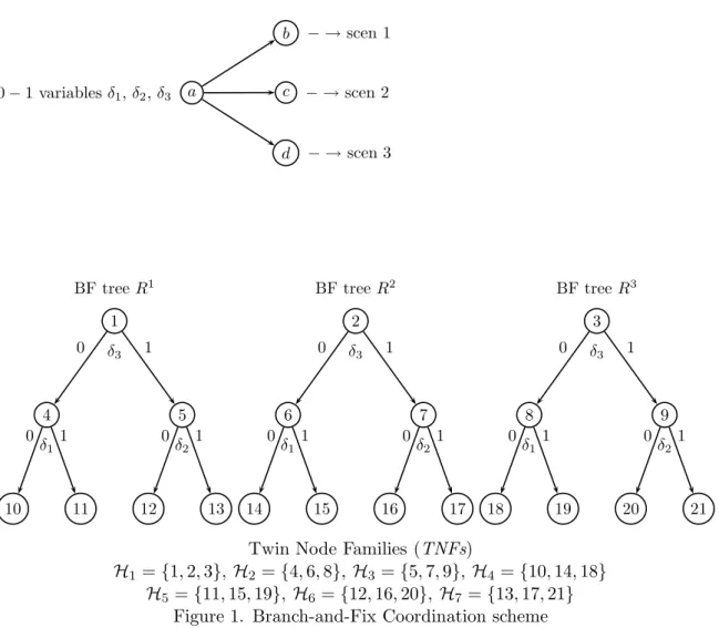
For the specialization of the BFC approach to solving problem(29), let Rω denote the BF tree associated with scenario ω, and Gω the set of active nodes in Rω, ω ∈Ω. Any two active nodes, say, g ∈ Gω and g ∈ Gω are said to betwin nodes if either they are the root nodes or the paths fromtheroot nodes to each of themin their own BF trees Rω and Rω, respectively, have branched on or fixed to the same 0–1 values for the same variablesδ_iω and δω_i,for ω, ω ∈ Ω, i∈ I. A Twin Node Family (TNF), say, H_f is a set of nodes, such that any one is atwin node to all the other members of the family, for f ∈ F, whereF is the set

0−1 variablesδ₁,δ₂,δ₃ a b − →scen 1 c − →scen 2 d − →scen 3 1 δ₃ BF tree R1 4 δ₁ 0 10 0 11 1 5 δ₂ 1 12 0 13 1 2 δ₃ BF treeR2 6 δ₁ 0 14 0 15 1 7 δ₂ 1 16 0 17 1 3 δ₃ BF treeR3 8 δ₁ 0 18 0 19 1 9 δ₂ 1 20 0 21 1

Twin Node Families (TNFs)

H1 ={1,2,3},H₂ ={4,6,8},H₃ ={5,7,9},H₄ ={10,14,18}

H5={11,15,19},H6 ={12,16,20}, H7={13,17,21}

Figure 1. Branch-and-Fix Coordination scheme

of TNFs. Note that g, g ∈ H_f for any family f ∈ F implies that ω = ω for g ∈ Gω and g ∈ Gω, ω, ω ∈ Ω. A TNF integer set is a a set of integer BF nodes, one per each tree, where thenonanticipativity constraints (27) of the 0–1 variables are satisfied.

Let us consider the scenario tree and the BFtrees shown in Figure 1, where δ_i gives the generic notation for the variables δ_iω, ∀ω ∈Ω. Notice that the first TNFto be used is H₁. Based on the LP optimal solution of the models (30) attached to the nodes in H₁, let us assume that the selected branching variable isδ₃ and, so, the nodes 4 and 5,6 and 7,and 8 and 9 are created. The newTNFs areH₂= (4,6,8) andH₃ = (5,7,9), and so forth.

It is clear that the relaxation of the nonanticipativity constraints (27) is not required for all pairs of scenarios in order to obtain computational efficiency. So, the number of scenarios to consider in a given model basically depends on the dimensions of the scenario related model (30) (i.e, the parameters |I| and t_i,∀i∈ I). The criterion for scenario clustering in the sets, say, Ω₁, . . . ,Ω_q, whereq is the number ofclustersto consider, could be alternatively based on the smallest internal deviation of the uncertain parameter (i.e., the interest rate rω_t, ∀t ∈ T), the greatest deviation, etc. The determination of the most efficient criterion

is instance dependent. In any case, notice that Ω_p∩Ω_p = ∅, p, p = 1, . . . , q : p = p and Ω = ∪q_p=1Ω_p. The specific measure for quantifying the deviation of the interest rate path for any two scenarios is also another instance dependent element. In any case, by slightly abusing the previous notation, the problemto consider for the scenario cluster p= 1, . . . , q can be expressed as follows,

Z_IPp = m in ω∈Ωp wω|yω| s.t. e δp _{≤ b1} A₂ δp = b_{2 δ}p _{∈ {0,1}}n −I_xδp +I_xxp ≤ 0 −I_xδp _+I xxp ≥ 0 e xp = b₃ aω₄ xp ≥ bω₄ ∀ω∈Ω_p A₅ωxp _+Bω_sω _{= b}ω 5 ∀ω∈Ωp s≤ I_s sω ≤ s ∀ω∈Ω_p aω₆xp +yω = bω₆ ∀ω∈Ω_p aω₇xp +zω = bω₇ ∀ω∈Ω_p |zω_{| ≤ z ∀ω∈Ω} p aω₈xp +vω = bω₈ ∀ω∈Ω_p |vω| ≤ v ∀ω∈Ω_p. (31)

Theq problems (31) are linked by the nonanticipativity constraints

δp_i −δp_i = 0 (32)

xp_i −xp_i = 0, (33)

∀i∈ I, p, p = 1, . . . , q:p=p.

3.2 All x–variables alone. Benders Decomposition scheme

By slightly abusing the notation, let the following represent theLP model after fixing in model (26) theδ–variables to the 0–1 values related to a given TNFinteger set. In the new model,x1 will denote the vector of thex–variables whose relatedδ–variables have taken the value 1, and the pair (x1, x1) gives the related lower and upper bounds.

Z_LPT N F = m in

ω∈Ω

s.t. e x1 = b₃ aω₄ x1 ≥ bω₄ ∀ω∈Ω x1≤ x1 ≤ x1 A₅ωx1 +Bωsω = b₅ ∀ω∈Ω s≤ I_s sω ≤ s ∀ω∈Ω aω₆x1 +yω = bω₆ ∀ω∈Ω aω₇x1 +zω = bω₇ ∀ω∈Ω |zω| ≤ z ∀ω∈Ω aω₈x1 +vω = bω₈ ∀ω∈Ω |vω| ≤ v ∀ω ∈Ω. (34)

By assuming that the x1–variables are the complicatingones and replacing the free vari-ables yω, zω and vω with y₁ω− yω₂, zω₁− z₂ω and vω₁− v₂ω, respectively, for yω₁, y₂ω, z₁ω, z₂ω v₁ω, v₂ω≥0, the original program(34) can be expressed

min x Fx s.t. e x1 = b₃ aω₄x1 ≥ bω₄ ∀ω∈Ω x1 ≤ x1 ≤ x1, (35) where F_x = ω∈Ω wωF_xω (36) and F_xω= m in y₁ω+yω₂ s.t. Bωsω = b₅−Aω₅x1 yω₁ −yω₂ = bω₆ −aω₆x1 z₁ω−zω₂ = bω₇ −aω₇x1 zω 1 +zω2 ≤ z vω₁ −v₂ω = bω₈ −aω₈x1 vω₁ +v₂ω ≤ v s≤ I_ssω ≤ s y₁ω, yω₂, z₁ω, zω₂, v₁ω, vω₂ ≥ 0. (37)

The dual of the primalLP problem(37) can be expressed F_xω = m ax (b₅−Aω₅x1)Tµω₅ + (bω₆ −a₆ωx1)µω₆ + (bω₇ −aω₇x1)µω₇ −zλω+ (bω₈ −aω₈x1)µω₈ −vβω+sTαω₁ −sTαω₂ s.t. BωTµω₅ +I_sαω₁ −I_sαω₂ ≤ 0 −1≤ µω 6 ≤ 1 µω₇ −λω ≤ 0 µω₇ +λω ≥ 0 µω₈ −βω ≤ 0 µω₈ +βω ≥ 0 αω₁, αω₂, λω, βω ≥0 µω₅, µω₇, µω₈ unrestricted. (38)

Given the structure of the constraint matrix that defines the feasible region in problem (38), it can be decomposed into a series of independent subproblems, such that

F_xω=F_xω(µω₅, αω₁, αω₂) +F_xω(µ₆ω) +F_xω(µω₇, λω) +F_xω(µω₈, βω) ∀ω∈Ω, (39) where F_xω(µω₅, α₁ω, αω₂) = m ax (b₅−A₅ωx1)Tµω₅ +sTαω₁ −sTαω₂ s.t. BωTµω₅ +I_sαω₁ −I_sαω₂ ≤0 αω₁, αω₂ ≥0 µω₅ unrestricted, (40) F_xω(µω₆) = m ax (bω₆ −aω₆x1)µω₆ s.t. −1≤µω₆ ≤1, (41) F_xω(µω₇, λω) = m ax (bω₇ −aω₇x1)µω₇ −zλω s.t µω₇ −λω ≤0 µω₇ +λω ≥0 λω≥0 µω 7 unrestricted, (42) and Fω x(µω8, βω) = m ax (bω8 −aω8x1)µω8 −vβω s.t µω₈ −βω≤0 µω₈ +βω≥0 βω ≥0 µω₈ unrestricted. (43)

The assumption of feasibility in the original model (34) requires the feasibility of the primal problems (37)∀ω∈Ω for all feasible values of the vectorx1 in the model (34). So, by the Duality Theorem,F_xω in the model (38) and, then, F_x (36) have also finite values.

Let Jp and Jr denote the sets of the extreme points and extreme rays of the feasible region in each problem(38), respectively. And, let an extreme point fromJp and an extreme ray fromJr be denoted as follows,

ν_jω≡(µω₅, µω₆, µω₇, µω₈, αω₁, αω₂, λω, βω)_j ω∈Ω, j ∈ Jp∪ Jr. (44) The problem(38) for ω∈Ω is finite if and only if

−c_jωx1+k_jω ≤0 j∈ Jr, (45) where k_jω = [µω₅]t_jb₅+st[αω₁]_j−st[αω₂]_j+bω₆[µω₆]_j+bω₇[µω₇]_j−z[λω]_j+bω₈[µω₈]_j −v[βω]_j c ω j = [µω5]tjAω5 + [µω6]jaω6 + [µω7]jaω7 + [µω8]jaω8. (46)

We can outer linearize the infimal value function in (38), such that it can be expressed as max

j∈Jp

ω∈Ω

wω(−c_jωx1+k_jω). (47)

By expressing the infimal value function by the outer linearized dual functions (38) and lettingZ denote the smallest upper bound, the original problem (34) for the givenTwin Node Family(TNF) can be represented as follows,

Z_LPT N F = m inZ (48) s.t. e x1 =b₃ (49) aω₄x1≥bω₄,∀ω ∈Ω (50) x1 ≤x1 ≤x1 (51) Z ≥ ω∈Ω wω(−c_jωx1+k_jω), ∀j∈ Jp (52) −c_jωx1+kω_j ≤0 ∀ω∈Ω, j ∈ Jr. (53) The problem(48)-(53) is known as the BendersMaster Program, see Benders (1962). It is not efficient to compute all its extreme points and rays (if any) (44) and, on the other hand, very few induced cuts (52)-(53) are frequently active at its optimal solution. A necessary condition for the implementation of this procedure is that the feasible region defined by (49)-(51) be finite. So, the solution can be iteratively obtained by identifying extreme points and rays based–cuts fromthe optimization of the so-called Auxiliary Program (AP), and appending themto the so-called Relaxed Master Program (RMP) for its optimization. The RMP can be expressed as

Z = m inZ s.t. e x1 =b₃ aω₄x1≥bω₄ ∀ω∈Ω x1 ≤x1 ≤x1 (54) Z ≥ ω∈Ω wω(−c_jωx1+k_jω) ∀j∈ Jp −c_jωx1+k_jω ≤0 ∀ω∈Ω, j∈ Jr,

whereJp ⊆ Jp andJr⊆ Jrare the subsets of the extreme points and extreme rays already identified, respectively.

At the first iteration,RMPis only included by the submodel (48)-(51). TheAP is given by the model (38), whose value (39) is obtained by solving independently the models (40)-(43) for a given value, say,xˆ1 of the vector of thex1–variables. This value is the optimal solution in theRMPthat has been solved in the previous iteration, its solution value beingZ.

Notice that the primal infeasibility (i.e., dual unboundness) of the model (37) is detected for the vectorxˆ1 if there is a scenario whose model (40)-(43) is unbounded for that vector. In this case, by the Farkas’ lemma, there exists an extreme rayν_jω (44) such that ν_jωW ≤0 and −cω_jx1+kω_j >0, whereW is the matrix of the feasible region for the dual problem (38). Then, one feasible cutfromthe set (55) should be appended to theRMP, at least.

−cω_jx1+k_jω ≤0 ∀ω ∈Ω0, (55) where Ω0 gives the set of scenarios fromΩ whose related models (40)-(43) are unbounded, and (44) gives the corresponding extreme ray.

On the other hand, if all dual models (40)-(43), ∀ω ∈Ω are bounded for the vector xˆ1, letZ=F_xˆ denote the optimal value of the objective function (39) and (56) be theoptimality cutto be appended to theRMPifZ (39)> Z (54).

Z ≥

ω∈Ω

wω(−cω_jx1+kω_j), (56)

where (44) gives the corresponding extreme point as the AP optimal solution for the point _xˆ1_.

Notice that ifZ =Z thenxˆ1 is the optimal solution of the model (34), beingZ_LPT N F =Z.

3.3 All x–variables with fractional δ–variables. Benders Decomposition

scheme

By abusing again the notation let δf denote the vector of the δ–variables to be allowed to take fractional values,δ1 the vector of theδ–variables that have been fixed to one,x1f _the

vector of thex–variables whose relatedδ–variables do not take the value zero in model (34), and ef and Af₂ (res.,e1 and A1₂) the unit row vector and constraint matrix for the variables’

vectorδf (res., δ1). The model can be expressed as follows, Z_LPf = m in ω∈Ω wω|yω| s.t. e δf ≤ b₁−e1δ1 A₂ δf = b₂−A1₂δ1 _δf _∈[0,1]n −I_xδf +I_xx1f ≤ 0 −I_xδf +I_xx1f ≥ 0 e x1f _{= b3} aω₄ x1f ≥ bω₄ ∀ω∈Ω A₅ωx1f +Bωsω = b₅ ∀ω∈Ω s≤ I_s sω ≤ s ∀ω∈Ω aω 6x1f +yω = bω6 ∀ω∈Ω aω₇x1f +zω = bω₇ ∀ω∈Ω |zω| ≤ z ∀ω∈Ω aω₈x1f +vω = bω₈ ∀ω∈Ω |vω| ≤ v ∀ω∈Ω. (57)

By assuming that the δf– andx1f–variables are the complicating ones and replacing the free variablesyω, zω andvω withy₁ω−y₂ω, zω₁−z₂ω andv₁ω−v₂ω,respectively, fory₁ω, y₂ω, z₁ω, z₂ω v₁ω, v₂ω≥0 as above, the program(57) can be expressed as

min x Fx s.t. e δf ≤ b₁−e1δ1 A₂ δf _{= b2−A}1 2δ1 _δf _∈[0,1]n −I_xδf +I_xx1f ≤ 0 −I_xδf +I_xx1f ≥ 0 e x1f = b₃ aω₄x1f ≥ bω₄ ∀ω ∈Ω, (58) where F_x = ω∈Ω wωF_xω (59)

andF_xω can be expressed following the same rationale as in (37)–(47), but replacingx1 with x1f. Fromwhere it results that Z_LPf can be expressed as

s.t. e δf ≤ b₁−e1δ1 A₂ δf = b₂−A1₂δ1 _δf _∈[0,1]n −I_xδf +I_xx1f ≤ 0 −I_xδf +I_xx1f ≥ 0 e x1f = b₃ aω 4x1f ≥ bω4 ∀ω∈Ω Z ≥ _ω∈Ωwω(−c_jωx1f +kω_j) ∀j∈ Jp −c_jωx1f +k_jω ≤ 0 ∀ω∈Ω, j ∈ Jr. (60)

The problem(60) is the BendersMaster Program. TheRelaxed Master Program (RMP) can be expressed as Z = m inZ s.t. e δf ≤ b₁−e1δ1 A₂ δf = b₂−A1₂δ1 _δf _∈[0,1]n −I_xδf +I_xx1f ≤ 0 −I_xδf +I_xx1f ≥ 0 e x1f _{= b3} aω₄x1f ≥ bω₄ ∀ω∈Ω Z ≥ _ω∈Ωwω_(−cω j x1f +kωj) ∀j∈ J p −c_jωx1f +k_jω ≤ 0 ∀ω∈Ω, j ∈ Jr, (61)

where Jp ⊆ Jp _{and J}r _{⊆ J}r _{are the subsets of the extreme points and extreme rays,}

respectively. Again, the feasible region of the initial relaxed master program must be finite. The Auxiliary Problem(AP) is given by the model (38) whose value (39) is obtained by solving independently the models (40)-(43) but, now, replacing the vectorxˆ1 with the vector _xˆ1f_.

Thefeasibilityand theoptimality cuts fromAPto be appended toRMPare given by the constraints (55) and (56), respectively, where againxˆ1 is replaced withxˆ1f.

3.4 BFC implementation

Different BFCimplementations can be considered. We present the version that has been implemented for performing the computational experimentation reported in Section 5.

Notice that theδ– andx–variables have zero coefficients in the objective function (12). In fact the y–variables are the unique variables in the objective function. These variables give the residual values of the duration balance equation (21) of theMBS portfolio and liabilities under each scenario. So, there is not a clear criterion for assigning branching priorities to the δ–variables. We have chosen the model’s input order (i.e., a random order) as the branching priority.

Based on the same reason, the objective function value could not be a good indication for the node branching selection. So, we have chosen the depth first strategy for the TNF branching selection, having first “branching on the zeros” and after “branching on the ones” for the chosenδ–variable to satisfy thenonanticipativityconstraints (32) for the selectedTNF to branch.

Notice that aTNFcan be pruned due to any of the following reasons: (a) theLPrelaxation of the scenario-cluster model (31) attached to a given node member is infeasible, (b) there is not a guarantee that a better solution than theincumbent one can be obtained fromthe best descendantTNFinteger set (in our current implementation, it is based on its objective function value, also called solution value), (c) theLPmodel (34) attached to theTNFinteger set is infeasible or its solution value is not better than the solution value of theincumbent solution, in case that all δ–variables have already been branched on or fixed for the family, and (d) see below when there is someδ–variable in theTNFinteger set that has not yet been branched on, nor fixed.

Once aTNFhas been pruned, the same branching criterion allows one to perform either a “branching on the ones” (in case it has already been “branched on the zeros”) or abacktracking to the previous branchedTNF.

The solution to be obtained by solving the LP model (34) attached to a TNF integer set could be the incumbent solution. However, it does not necessarily mean that it should be pruned, except if all δ–variables have been branched on or fixed for the family, as it is said above. Otherwise, a better solution can still be obtained by branching on the non-yet branched on, nor fixed δ–variables. Let Z_LPT N F be the solution value in (34) that satisfies thenonanticipativity constraints (28) by fixing theδ–variables to their 0–1 values (where the constraints (27) are already satisfied). The family can be pruned if Z_LPT N F = Z_LPf , where Z_LPf is the solution value of model (57), where both constraint types are satisfied, but the non-yet branched on, nor fixedδ–variables are allowed to take fractional values. Notice that the solution space defined by model (34) is included in the space defined by model (57). In this case, there is no better solution than ZT N F

LP to be obtained fromthe descendantTNF

integer sets.

For presenting theBFCalgorithmto solve model (29), let the following additional notation be adopted:

Rp_{, BFtree for the scenario cluster p, for p= 1, . . . , q.}

LPp_{, LPrelaxation of the scenariocluster-related model (31) attached to a given node}

member from the BFtree Rp in the given TNF, forp= 1, . . . , q.

Z_LPp , solution value of the LP model LPp_{, forp= 1, . . . , q. By convention, let Z}p LP =

+∞ in case of infeasibility. Note: Z_LPp is the expected duration mismatching of the MBS portfolio and the liabilities over the scenarios incluster p, for theLP relaxation case.

Z_IP, lower bound of the solution value of the original model (29) to be obtained from the best descendant TNFinteger set for a given family. It will be computed asZ_IP =

p=1,...,qZLPp for any family, but the one included by the root nodes of the BF trees.

For the latter family, Z_IP is given by the LP relaxation of the original problem(26); the value is reported as Z_LP in the computational experience shown in section 5 when

computed in Step 1 below, and it is obtained by solving the problem (57), via Benders Decomposition, without fixing a priori any δ–variable.

By convention, Z_LPT N F = +∞, for the infeasible problem(34) related to a given TNF integer set, andZ_LPf = +∞, for the infeasible problems (57).

BFC Algorithm

Step 0: Initialize Z_IP := +∞.

Step 1: Solve theLPrelaxation of the original problem(26) and computeZ_IP.If there is anyδ–variable that takes a fractional value then goto Step 2. Otherwise, the optimal solution to the original problemhas been found and, so, Z_IP := Z_IP and stop.

Step 2: Initialize i:= 1 and goto Step 4.

Step 3: Reset i:=i+ 1.Ifi=|I|+ 1 then goto Step 8. Step 4: Branch δ_ip:= 0 and, so, fix xp_i := 0,∀p= 1, . . . , q.

Step 5: Solve the linear problems LPp,∀p= 1, . . . , q and computeZ_IP.

If Z_IP ≥Z_IP then goto Step 7. If there is any δ–variable that either takes fractional values or takes different values for some of the q scenario clustersthen goto Step 3. If all the x–variables take the same value for all scenario clusters p = 1, . . . , q then updateZ_IP := Z_IP and goto Step 7.

Step 6: Solve theLP model (34) to satisfy the constraints (33) for thex1–variables in the given TNFinteger set. Notice that the solution value is denoted by Z_LPT N F.

Update Z_IP := min{Z_LPT N F, Z_IP}. Ifi=|I| then goto Step 7.

Solve theLPmodel (57), where the fractionalδ–variables are the non-yet branched on, nor fixed in the current TNF. Notice that the solution value is denoted by Z_LPf . If Z_LPT N F =Z_LPf then goto Step 7, otherwise goto Step 3.

Step 7: Prune the branch.

If δp_i = 0,∀p= 1, . . . , q then goto Step 10. Step 8: Reset i:=i−1.

If i= 0 then stop, since the optimal solution Z_IP has been found. Step 9: If δp_i = 1, ∀p= 1, . . . , qthen goto Step 8.

Step 10: Branchδp_i := 1 and, so,x_i ≤xp_i ≤ x_i,∀p= 1, . . . , q. Goto Step 5.

4

Illustrative case

In this section we present an illustrative case, where we have |Ω|= 2 scenarios, |I|= 3 securities, |T | = 4 tim e periods, = 3 dedicated time periods and a maximum of b₁ = 2 securities in the portfolio. In spite of the small toy instance, the model (12)-(25) has 26 constraints, 24 variables (3 are 0–1 ones) and 90 nonzero elements in the constraint matrix. The interest rate path along the time horizon is as follows, in percentage: r₁1 = r₁2 = 6.3, r1₂ = 6.5,r₂2 = 6.1, r₃1= 7.5,r2₃ = 7.9,r₄1= 8.0, andr2₄ = 8.1. Objective function: Z_IP = m in 0.5y+1+ 0.5 y−1+ 0.5 y+2+ 0.5 y−2 Constraints: δ₁+δ₂+δ₃ ≤2 700δ₁−x₁ ≤0 400δ₂−x₂ ≤0 1000δ₃−x₃ ≤0 −1300 δ₁+x₁ ≤0 −1700 δ₂+x₂ ≤0 −2700 δ₃+x₃ ≤0 x₁+x₂+x₃ = 3000 0.936641 x₁+ 0.938030 x₂+ 0.937013x₃≥2788.769287 0.936293 x₁+ 0.937609 x₂+ 0.937256x₃≥2792.632813 −s1₁+ 0.252000 x₁+ 0.158500 x₂+ 0.336150 x₃ = 894 −s2₁+ 0.248800 x₁+ 0.154900 x₂+ 0.333310 x₃ = 894 1.065 s1₁−s1₂+ 0.420750 x₁+ 0.252500 x₂+ 0.340000 x₃ = 846 1.061 s2₁−s2₂+ 0.422390 x₁+ 0.255300 x₂+ 0.341600 x₃ = 846 1.075 s1₂−s1₃+ 0.410000 x₁+ 0.330800 x₂+ 0.400000 x₃ = 798 1.079 s2₂−s2₃+ 0.410000 x₁+ 0.330400 x₂+ 0.400000 x₃ = 798 2.102381 x₁+ 2.767783 x₂+ 2.009360x₃−y+1+y−1= 6511.689941 2.105035 x₁+ 2.771116 x₂+ 2.011282x₃−y+2+y−2= 6516.945800 2.102381x₁+ 2.767783 x₂+ 2.009360 x₃−3000 z+1+ 3000z−1= 6800.824707 2.105035x₁+ 2.771116 x₂+ 2.011282 x₃−3000 z+2+ 3000z−2= 6808.942871 z+1+z−1 ≤0.566735 z+2+z−2 ≤0.566735 0.936641 x₁+ 0.938030 x₂+ 0.937013x₃−3000 v+1+ 3000v−1= 2811.262939 0.936293 x₁+ 0.937609 x₂+ 0.937256x₃−3000 v+2+ 3000v−2= 2810.480957 v+1+v−1 ≤0.234272 v+2+v−2 ≤0.234272 δ₁, δ₂, δ₃∈ {0,1} 22.5≤s1₁, s2₁ ≤2250 15≤s1₂, s2₂ ≤1500 7.5≤s1₃, s2₃ ≤750 y+ω, y−ω, z+ω, z−ω, v+ω, v−ω ≥0,∀ω= 1,2 (62)