a Neural Network Enhanced Hamiltonian
Markov Chain Monte Carlo Sampler
Thomas Yu 1, Marco Pizzolato 1, Gabriel Girard2, Jonathan Rafael-Patino1, Erick Jorge Canales-Rodr´ıguez1,2,3,4, and Jean-Philippe
Thiran1,2,5
1 Signal Processing Lab (LTS5), ´Ecole Polytechnique F´ed´erale de Lausanne,
Lausanne, Switzerland
[email protected], [email protected]
2
Department of Radiology, Centre Hospitalier Universitaire Vaudois (CHUV), Lausanne, Switzerland
3 FIDMAG Germanes Hospital`aries, Sant Boi de Llobregat, Barcelona, Spain 4
Mental Health Research Networking Center (CIBERSAM), Madrid, Spain
5 University of Lausanne, Lausanne, Switzerland
Abstract. Probabilistic parameter estimation in model fitting runs the gamut from maximum likelihood or maximum a posteriori point esti-mates from optimization to Markov Chain Monte Carlo (MCMC) sam-pling. The latter, while more computationally intensive, generally pro-vides a better characterization of the underlying parameter distribution than that of point estimates. However, in order to efficiently explore dis-tributions, MCMC methods ideally require generating uncorrelated sam-ples while also preserving reasonable acceptance probabilities; this be-comes particularly important in problematic regions of parameter space. In this paper, we extend a recently proposed Hamiltonian MCMC sam-pler parametrized by neural networks (L2HMC) by modifying the loss function to jointly optimize the distance between samples and the ac-ceptance probability such that it is stable and efficient. We apply this enhanced sampler to parameter estimation in a recently proposed MRI model, the multi-echo spherical mean technique. We show that it gen-erally outperforms the state of the art Hamiltonian No-U-Turn (NUTS) sampler, L2HMC, and a least squares fitting in terms of accuracy and precision, also enabling the generation of more informative parameter posterior distributions. This illustrates the potential of machine learning enhanced samplers for improving probabilistic parameter estimation for medical imaging applications.
Keywords: Markov Chain Monte Carlo·Hamiltonian MCMC Sampler ·Magnetic Resonance Imaging·Optimization·Parameter Estimation.
1
Introduction
Given a data vectors∈Rdgenerated from varying an independent experimental
explain the data, probabilistic parameter estimation constructs a probabilistic model for the data and views the problem as inferring the parameters of a prob-ability distribution [17]. For example, one can define the likelihood of the data given fixed parameters by treating each data point as an independent sample from a Gaussian distribution with mean at the model evaluated at the corre-sponding v,x and with a variance coming from the measurement noise. Using Bayes’ theorem, the posterior probability distribution of the parameters given the data is proportional to the product of the likelihood function and the priors on the parameters: p(x|s)∝p(s|x)p(x), (1) where, p(s|x) =N(M(x,v), σ2) = d Y i=1 1 √ 2πσ2exp( (si−M(x,vi))2 2σ2 ), (2)
and σ2 denotes the noise variance. The prior distribution p(x) encodes con-straints such as sum concon-straints or upper/lower bounds through, for example, Dirichlet and uniform distributions [1]. An immediate candidate for a parameter estimate is then the maximum a posteriori (MAP) point estimate
x∗= arg max
x
p(x|s). (3) This reduces the parameter estimation to an optimization problem. However, there are two potential problems with this point estimate. First, the general problems of uniqueness and feasibility of optimization, i.e. finding the MAP esti-mate. Second, the underlying assumption of this point estimate is that the mode is a good representation of the underlying probability distribution. Intuitively, we can see the truth of this assumption for many commonly used distributions in three or less dimensions e.g. normal or exponential. However, this assumption can fail as the dimensionality and complexity of the distribution increases due to the geometry of high dimensional spaces [3] and the concentration of measure phenomenon [3, 14]. Hence, inferring the parameters of a probabilistic model of high dimension and/or complexity through a mode point estimate can lead to spurious results. One approach to handle these issues is to first characterize the posterior distribution with Markov Chain Monte Carlo (MCMC) techniques [9] by sampling from the posterior distribution. One can then, as an example, use the mode, mean, median, etc. of the marginal posterior distributions of the pa-rameters for the parameter estimate. In this paper, we use the expectation of each parameter over its marginal posterior, approximated by
x∗≈ 1 N N X i xi, (4)
where the subscriptidenotes one of the N samples.
The contributions of this paper are, first, to extend a Hamiltonian MCMC sampler parametrized with neural networks proposed in [15] . We modify the
loss function to balance acceptance probability and mixing such that both fast mixing and stable exploration of problematic regions of state space are possible. Second, we apply our extended sampler to estimate the parameters of a recently proposed MRI model and compare it to a least squares fitting and application of two state of the art Hamiltonian samplers.
2
Related Work
2.1 Hamiltonian Markov Chain Monte Carlo
In the following, we denote the posterior distribution from which we want to sample asp(x) with x∈Rn being the state variables. MCMC methods sample
from the posterior by generating a sequence of samples where each new sample xt is generated from the previous samplext−1 according to a transition distri-butionT(xt|xt−1) [4]. In order for the posterior to be the unique distribution to which this sequence converges, the transition distribution must satisfy ergodic-ity, which can usually be safely assumed, and an invariance property which is usually shown by proving a property called detailed balancep(xt)T(xt−1|xt) =
p(xt−1)T(xt|xt−1).
One well known way to construct a transition satisfying detailed balance called the Metropolis-Hastings algorithm [9] is as follows: given a proposal dis-tribution q(x0|xt−1), sample a candidate x0; then, accept x0 with probability A(x0|xt−1) = min(1, p(x 0)q(x t−1|x0) p(xt−1)q(x0|xt−1)). If accepted, xt = x 0. If rejected, x t =
xt−1. However, even if a sampler satisfies these properties, the convergence is only proven asymptotically [4]. The typical procedure is to first have a burn-in stage where the sampler is run for some amount of steps burn-in order for it to converge. Then, the actual sampling begins, with the burn-in samples being discarded [4].
For efficient exploration, the samples should ideally be uncorrelated, which can be accomplished by large distances between samples in the sample space, i.e. mixing. Autocorrelation analysis using multiple chains of samples can be used as a rough measure of how many samples are necessary. We emphasize that a balance must be found between the acceptance probability and the mixing; acceptance probabilities which are very high can mean the samples are very close/correlated and large distances between samples can lead to only a small number of samples being accepted. One powerful MCMC method which scales with the dimensionality and complexity of the posterior is Hamiltonian MCMC (HMCMC) [6]. In HMCMC, one generates proposal samples by integrating along trajectories of a Hamiltonian dynamical system constructed from combining the posterior distribution of interest with a momentum distribution. This is then followed by the Metropolis acceptance step to yield a new sample. Formally a
joint distribution is constructed with state variables (x,p): pH(x,p)∝exp(−U(x)−K(p)), (5) p(x)∝exp(−U(x)), (6) K(p) =1 2p Tp, (7)
where we omit a normalizing constant andpare the momentum variables which are added. This form is motivated from statistical physics by the canonical dis-tribution of energy states of a system, whereU andK denote the potential and kinetic energy respectively, and the Hamiltonian (total energy) isH =U+K[6]. HMCMC samples frompH(x,p), and we can obtain the marginal distribution of xfrom the samples.H defines a dynamical system, which is a set of differential equations used to evolvex,pforward in time from an initial sample.
In practice, these equations are integrated numerically, characterized by a step sizeand a number of stepsLsuch thatLis the time period over which a sample trajectory is evolved. The most common numerical scheme is the leapfrog scheme, which we write below for one time step with initial condition (x,p) and result (x0,p0). p12 =p− 2∂xU(x),x 0 =x+p1 2,p0 =p− 2∂xU(x 0). (8)
Given an initial x0, an initial momentum p0 is sampled from a distribution,
usually a standard Gaussian [4]. The proposed sample from running the dy-namics, (x0,p0), is then accepted in a Metropolis-Hastings step with probability α = min(1, exp(−U(x)−12p
Tp)
exp(−U(x0)−12p0Tp0)). Ideally, this procedure is then repeated un-til the convergence of the samples to the distribution, with the output of each proposal becoming the new initial sample. The main advantage of HMCMC is that it generally proposes samples which are far away from the initial sample, thus efficiently exploring the posterior, while maintaining reasonable acceptance probabilities [4]. A state of the art HMCMC sampler called the No U Turn Sam-pler (NUTS) [10] improves on standard HMCMC by adaptively tuning L, to manage the distance between samples and acceptance probability. HMCMC can perform poorly in certain circumstances, in particular, in highly curved sample spaces such as those that might arise in the posteriors derived from parameter estimation of complex models [8].
2.2 L2HMC
Levy et. al. [15] recently proposed a framework called L2HMC which parametrizes the standard HMCMC sampler with a neural network and maximizes the ex-pected distance between samples through minimization of a loss function which rewards large expected squared distances between samples. Furthermore, the parametrization is carefully tailored to preserve detailed balance and have a tractable Jacobian for the correction of the acceptance probability due to the
potential non-volume preserving dynamics. The algorithm of L2HMC is struc-turally similar to standard HMCMC, but modifications are made to the proposal stage. First, for each step t, 1 ≤t ≤L, a random binary mask mt ∈ {0,1}n is
constructed such that approximately half of the entries of the mask are 1. The conjugate mask is denoted as mc
t. Instead of updating x in one step
accord-ing to the classical algorithm, the update is split into two steps each updataccord-ing only the variables ofxcorresponding tomt, mct separately. These are denoted as
xmt =xmt andxmct =xm c
t respectively, whereis the component-wise
multiplication operator. Each update equation is modified with scaling factors for each term depending on only variables which are not being updated. Con-cretely, letζ1= (x, ∂xU(x0), t). Thenpis first updated according to
p12 =pexp(
2Sp(ζ1))−
2∂xU(x)exp(Qp(ζ1)) +Tp(ζ1), (9) where Sp, Qp, Tp :R2n+1 →Rn are scaling functions parameterized by a neural
network. Letζ2= (xmc
t,p, t) andζ3= (x 1 2
mt,p, t). Thenxis updated according to x12 =xmc t +mt h xexp(Sx(ζ2)) +(p 1 2exp(Qx(ζ2)) +Tx(ζ2)) i , (10) x0=xmt+m c t h xexp(Sx(ζ3)) +(p 1 2 exp(Qx(ζ3)) +Tx(ζ3)) i , (11) where Sx, Qx, Tx : R2n+1 → Rn are also scaling functions parameterized by a
neural network. Finally, letζ4= (x0, ∂xU(x0), t):
p0=p12 exp( 2Sp(ζ4))− 2∂xU(x 0)exp(Q p(ζ4)) +Tp(ζ4). (12)
These learned scaling functions, structured as a two layer neural network, can allow the sampler to learn, for example, how to carefully navigate regions of high curvature in the parameter space rather than having to manipulate and L to accomplish this. As in NUTS [10], the time reversed version of the above dynamics can also be used to propose samples, and L2HMC takes a random combination of the forward and backward dynamics proposal as the final pro-posal [15]. Letθ be the vector of parameters of the above functions. After each complete cycle of proposal and acceptance, the loss function is optimized using Adam [12]. Concretely, let ξ= (x, p) be the initial sample, andξ0 = (x0, p0) be the sample after the acceptance step. Letδ(ξ, ξ0) =kx−x0k2
2andA(ξ0, ξ) denote the acceptance probability. Then the loss functionL(θ) used is
L(θ) =Ep(ξ) −δ(ξ, ξ 0)A(ξ0, ξ) λ2 + λ2 δ(ξ, ξ0)A(ξ0, ξ) , (13) where the expectation is taken over the batch of samples over which the training is taking place. λ is the typical length scale of the distribution, which Levy et. al. set in the case of a multivariate normal distribution, as the smallest standard deviation in the covariance matrix. For simplicity, in eq. 13, we omit an additional term with identical form as above [15] designed to enhance burn-in by usburn-ing an arbitary proposal distribution. Fig 1 shows a flowchart of the algorithm of sampling with the neural network parametrization.
Fig. 1.Flowchart of the training algorithm for neural network parametrization of HM-CMC. The components of the algorithm are very similar to standard HMCMC; how-ever, the differences lie in the altered dynamics/proposal stage and the update of the neural network parameters after each step. When sampling, the network parameters are fixed at the last training values.
3
Methods
3.1 Neural Network Enhanced Hamiltonian MC (NNEHMC) The first contribution of this paper is to extend L2HMC by augmenting the loss function to balance acceptance probability and the distance between samples. LetAHM C(ξ0, ξ) denote the acceptance probability used in standard HMCMC.
We introduce the loss function
LN N EHM C(θ) =
Ep(ξ)[−δ(ξ, ξ0)A(ξ0, ξ)−βAHM C(ξ0, ξ)]. (14)
We removed the reciprocal distance term as it did not meaningfully change the dynamics of the sampling in the distributions we considered. Further, we do not integrate the time reversed dynamics in our sampling. We argue that this form of loss function more faithfully and naturally enhances the desirable properties of Hamiltonian dynamics. In theory, Hamiltonian dynamics preserve energy along trajectories; hence, since the probability of a sample is proportional to exp(−H), the acceptance probability is always 1 [4]. However, the introduction of numerical integration causes violation of this property; nonetheless HMCMC still, generally, provides high acceptance rates, with additional tuning possible through changing orL. One can view this tuning as reducing the error of the leapfrog scheme such that the numerical integration gets closer and closer to the theoretical Hamiltonian dynamics with its property of preserving energy. However, the dynamics of L2HMC is no longer a numerical approximation of Hamiltonian dynamics due to the scaling terms. Hence, while it is valid as an MCMC sampler, there is no theoretical basis for the sampler to produce samples with high acceptance probabilities which are largely independent of the squared distance as in standard HMCMC.
As a way of both inducing the sampler to remain close to Hamiltonian dynam-ics and balancing the acceptance probability and mixing, we add the negative standard HMCMC acceptance probability in the loss function, with the pa-rameterβ enforcing the tradeoff between it and the negative expected squared distance. We argue that this loss function can lead to two desirable properties. First, it could lead to faster mixing and faster convergence than in L2HMC since, from the beginning, it can balance learning the standard, approximately energy preserving Hamiltonian dynamics with opportunities to move great distances. One can interpret the additional term as enforcing approximate conformity, in some sense, to Hamiltonian dynamics, mediated by β. Second, crucial for pa-rameter estimation, we argue that this term helps to keep the sampler stable when exploring high curvature regions. In these regions, the acceptance proba-bility can drop to zero easily due to large distance steps and numerical issues can develop [8]. The acceptance probability of the neural network parametrized sampler differs from the classical acceptance by the Jacobian of the new, scaled dynamics, which is identically 1 in the standard case. Hence, if the standard acceptance probability is the dominant term, it can still enforce high acceptance probabilities for the sampler. We thus treat the neural network as an enhance-ment that allows the sampler to learn ”approximate” Hamiltonian dynamics which can balance and enhance the desirable properties of HMCMC while learn-ing to minimize its weaknesses. We henceforth refer to our sampler as Neural Network Enhanced Hamiltonian MC (NNEHMC).
In the results, we compare the performance of NNEHMC and L2HMC on a toy distribution also tested in [15]. The distribution is a strongly correlated 2-D Normal distribution with mean zero, and a covariance matrix obtained from diag(100,0.1) rotated by 45 degrees. For both samplers, we use the same = 0.1, L= 10, initialize with the same 200 samples, train in batches of 200 samples for 5000 steps, then fix the neural network parameters and sample 200 chains for 2000 steps using the trained sampler [15]. We tune β in NNEHMC by looking at the autocorrelation analysis and the acceptance probabilities. We setλ= 0.1 as is done in [15]. We compare the two samplers by the autocorrelation of the samples as well as the effective sample size derived from the autocorrelation, which can be seen as a measure of how many of the samples are ”useful” for inference [4].
3.2 Biophysical Parameter Estimation
The second contribution of this paper to apply NNEHMC to biophysical pa-rameter estimation in a recently proposed MRI model, the Multi Echo Spherical Mean Technique (MESMT) [5].
Multi Echo Spherical Mean Technique (MESMT). MRI Diffusometry and T2 relaxometry can be combined into a multi-modal analysis which jointly estimates diffusivities, T2’s, and water volume fractions of different tissue com-partments. The extended spherical mean technique (SMT) framework introduced
by [5] is one example of this, generalizing the diffusion MRI model SMT [11] by including the effects of changing the echo timeTEin the acquisition on the MRI
signal and using the additional information to simultaneously estimate theT2’s and diffusivities of the compartments in brain white matter. The model signal is a function ofb andTE. For givenb, TE
M odel(TE, b,x) =vIexp( −TE TI 2 ) √ πerf(pbλ k) 2p bλk +vEexp( −TE TE 2 ) exp(−bλ⊥) √ πerf(p b(λk−λ⊥)) 2p b(λk−λ⊥) +vCSFexp( −TE T2csf) exp(−bDcsf),
where vI, vE, vCSF are the volume fractions of the intra-axonal, extra-axonal,
and cerebrospinal fluid (CSF) compartments respectively,λk, λ⊥ are the parallel and perpendicular diffusivities. The likelihood of this model is constructed as in the introduction. In the fitting, we fix the values of T2csf = 2s and Dcsf =
0.003mms2 at those of free water [11, 16], but we allowvCSF to be free.
Using our proposed sampler, we can bound the T2’s and diffusivities based on prior physical knowledge [11, 16] so we use uniform priors as follows:
TI 2 ∼ U(5ms,200ms),T2E∼ U(5ms,100ms),λk∼ U(0.0005mm 2 s ,0.003 mm2 s ), λ⊥∼ U(0.0001mm 2 s ,0.0005 mm2 s ).
Experimental Setup. We simulate three datasets using three differentTE0s= 50,75,100ms, with threeb = 300,2150,4000s/mm2 values per dataset, and fit them simultaneously. The ground truth parameters are as follows:vI = 0.5, vE=
0.3, vCSF = 0.2, λk = 0.0015mm 2 s , λ⊥ = 0.0002 mm2 s , T I 2 = 140ms, T2E = 70ms. Since the volume fractions must sum to one, we use a 3D, symmetric Dirich-let prior for the volumes: (vI, vE, vCSF)∼Dir(1.0,1.0,1.0). We generated one
hundred signals from the ground truth parameters by adding one hundred re-alizations of Gaussian noise with a standard deviation of σ = 1201 . We simu-lated many instances of a typical diffusion acquisition using Dmipy [7] with a mean SNR of 20 on the b0 data, then performed spherical averaging on each instance. The standard deviation of the resulting signals over the instances was estimated to be around 1201 , which motivates our setting ofσ. We then estimated the parameters over each signal using NUTS, L2HMC, and NNEHMC within the Bayesian framework described in Section 3.2. We also show a fitting using constrained least squares (LSQ). We imposed the same constraints in both the probabilistic and deterministic fittings. We initialize NUTS with a variational inference estimate [13], and use 1000 samples for burn-in and 1000 samples for inference. We initialize L2HMC and NNEHMC with the first 50 samples of the NUTS burn-in, train on batches of 50 samples for 1000 steps, then fix the param-eters of the network and use the trained sampler to generate 1000 samples for inference. We set λ=σ, since it is roughly the length scale of the distribution.
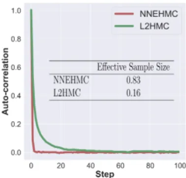
Fig. 2. Plot of the average autocorrelation of 200 chains of length 2000 for L2HMC and NNEHMC with the corresponding effective sample size. The autocorrelation and effective sample size are calculated as in [15]. We see that NNEHMC mixes faster in sampling steps and has a larger effective sample size.
In the results, we report the relative absolute error as follows: letting g denote the ground truth parameter andeas the estimate, the relative absolute error is computed as |g−e|/g. We note that we scale b by 10e−2 and the diffusivities by 10e2 in the sampling and results.
4
Results and Discussion
4.1 Strongly Correlated GaussianIn Fig 2, we show the average autocorrelation of the samples over 50 chains from sampling the strongly correlated Gaussian as a function of steps in the chain as well as a table with the effective sample sizes derived from the autocor-relation. We note that NNEHMC mixes faster and has an effective sample size almost eight times larger than that of L2HMC. Further, on the same computer, NNEHMC requires 179s of computation time while L2HMC requires 1561s. This is mostly because NNEHMC does not use the time reversed dynamics. In cases with tractable distributions and derivatives one can also speed up the sampling by using GPU computation [2].
4.2 Multi Echo Spherical Mean Technique (MESMT)
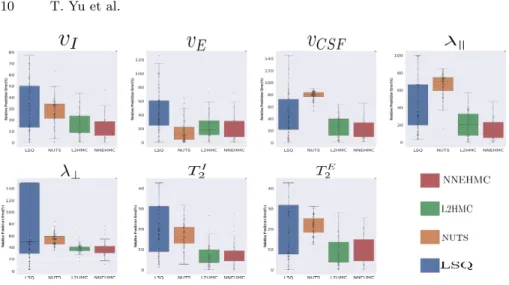
In Fig. 3, 4, we show the relative absolute error and an example of the marginal posterior probability distributions produced by the MCMC samplers.
We can see that, in general, the MCMC samplers are more accurate and pre-cise than the least squares fitting. However, we see that NNEHMC and L2HMC significantly outperform NUTS in estimating volume fractions and λk, even
Fig. 3. Box plots of relative absolute errors from ground truth using least squares (blue), NUTS (orange), L2HMC (green), and NNEHMC (red). We note that in general, NNEHMC has the lowest mean error and variance. Further, NUTS has significant issues in the estimation ofλk and the volume fractions, which is not observed in NNEHMC
or L2HMC.
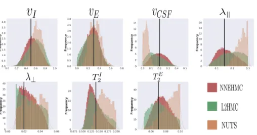
though they all start from the same initialization. Inspection of the probabil-ity distributions reveals that NUTS gives distributions biased away from the ground truth for these parameters. Furthermore, we note that NNEHMC gener-ally outperforms L2HMC regarding the accuracy and variance of the estimates. Unlike in the toy example, where we knew the precise mean and variance of the distribution, we can only compute an approximate autocorrelation analysis in this case. We obtained an effective sample size of 1.5e−3 for NNEHMC and 1.9e−3 for L2HMC. However, the mean computation times for a single signal are 280sfor NNEHMC and 443sfor L2HMC.
Furthermore we emphasize that using L2HMC on this model is numerically unstable.By changing the random seed in our implementation, 18 out of the 100 trials with L2HMC either decline to and remain at zero acceptance probability for all chains by the end of training or encounter numerical errors (NaN, infinities). This can happen, for instance, if the proposal samples move too far away. NNEHMC was robust to such changes. We do not consider these results in the analysis since they are invalid for parameter estimation and would artificially bias the results for L2HMC negatively. In order for NUTS not to develop similar numerical issues, we had to set a desired acceptance probability of 99%. It is probable that the poor results of NUTS stem, in part, from inefficient sampling due to a highly curved parameter space which the adaptive tuning could not overcome. Thus, we can see that the parametrization with a neural network can enable efficient sampling of problematic regions in parameter space; however, regularization with an acceptance probability term is needed for stability.
Fig. 4.Representative plots of the marginal probability distributions for each param-eter, where the black vertical line denotes the ground truth value. We can see that NNEHMC provides informative posterior distributions from which inference seems justified, while NUTS provides quasi-uniform distributions and distributions biased towards the parameter bounds.
5
Conclusion
In this paper, we have proposed and tested a parametrization of Hamiltonian MCMC with a neural network (NNEHMC) which jointly optimizes sample accep-tance probability and disaccep-tances between successive samples in order to efficiently and stably sample probability distributions, particularly in regions of parameter space with high curvature. Such regions frequently occur in the probabilistic es-timation of parameters in bio-physical models since the posterior distributions are parametrized, in part, by highly nonlinear models. We show on a recently proposed MRI model that the neural network enhancement provides parame-ter estimates which are more accurate and precise than those given by a least squares fitting and the state of the art NUTS and L2HMC samplers; in addition NNEHMC provides more numerically stable sampling than NUTS or L2HMC. Furthermore, we show that the neural network parametrization provides qualita-tively different and more informative posterior distributions than those produced from NUTS; NNEHMC can produce posterior distributions which are Gaussian-like centered near the correct parameter values. This highlights the potential of augmenting MCMC methods with neural networks to improve probabilistic estimation of parameters in biophysical models.
Acknowledgements. Thomas Yu is supported by the European Union’s Hori-zon 2020 program under the Marie Sklodowska-Curie project TRABIT (agree-ment No 765148). Marco Pizzolato is supported by the SNSF under Sinergia
CRSII5 170873. This work is also supported by the Center for Biomedical Imag-ing (CIBM) of the Universities of Geneva and Lausanne and the EPFL as well as the foundations of Leenaards and Louis-Jeantet.
References
1. Balakrishnan, N., Nevzorov, V.B.: A Primer on Statistical Distributions. John Wiley & Sons (2004)
2. Beam, A.L., Ghosh, S.K., Doyle, J.: Fast Hamiltonian Monte Carlo using GPU Computing. Journal of Computational and Graphical Statistics 25(2), 536–548 (2016)
3. Betancourt, M.: A conceptual introduction to Hamiltonian Monte Carlo. arXiv preprint arXiv:1701.02434 (2017)
4. Brooks, S., Gelman, A., Jones, G., Meng, X.L.: Handbook of Markov Chain Monte Carlo. CRC press (2011)
5. Canales Rodriguez, E.J., Pizzolato, M., Aleman-Gomez, Y., Kunz, N., Pot, C., Thiran, J.P., Daducci, A.: Unified multi-modal characterization of microstructural parameters of brain tissue using diffusion MRI and multi-echo T2 data. In: Joint Annual Meeting ISMRM-ESMRMB (2018)
6. Duane, S., Kennedy, A.D., Pendleton, B.J., Roweth, D.: Hybrid Monte Carlo. Physics Letters B195(2), 216–222 (1987)
7. Fick, R., Wassermann, D., Deriche, R.: Mipy: An Open-Source Framework to im-prove reproducibility in Brain Microstructure Imaging. In: OHBM 2018-Human Brain Mapping. pp. 1–4 (2018)
8. Girolami, M., Calderhead, B.: Riemann Manifold Langevin and Hamiltonian Monte Carlo Methods. Journal of the Royal Statistical Society: Series B (Statistical Methodology)73(2), 123–214 (2011)
9. Hastings, W.K.: Monte Carlo sampling methods using Markov chains and their applications (1970)
10. Hoffman, M.D., Gelman, A.: The No-U-Turn Sampler: Adaptively Setting Path Lengths in Hamiltonian Monte Carlo. Journal of Machine Learning Research15(1), 1593–1623 (2014)
11. Kaden, E., Kelm, N.D., Carson, R.P., Does, M.D., Alexander, D.C.: Multi-compartment microscopic diffusion imaging. NeuroImage139, 346–359 (2016) 12. Kingma, D.P., Ba, J.: Adam: A Method for Stochastic Optimization. arXiv preprint
arXiv:1412.6980 (2014)
13. Kucukelbir, A., Tran, D., Ranganath, R., Gelman, A., Blei, D.M.: Automatic Differentiation Variational Inference. The Journal of Machine Learning Research
18(1), 430–474 (2017)
14. Ledoux, M.: The Concentration of Measure Phenomenon. No. 89, American Math-ematical Soc. (2001)
15. Levy, D., Hoffman, M.D., Sohl-Dickstein, J.: Generalizing Hamiltonian Monte Carlo with Neural Networks. arXiv preprint arXiv:1711.09268 (2017)
16. MacKay, A.L., Laule, C.: Magnetic Resonance of Myelin Water: An in vivo Marker for Myelin. Brain Plasticity2(1), 71–91 (2016)
17. Sengijpta, S.K.: Fundamentals of Statistical Signal Processing: Estimation theory (1995)