Industrial and Manufacturing Systems Engineering
Publications Industrial and Manufacturing Systems Engineering 11-2018
Statistical reliability of wind power scenarios and
stochastic unit commitment cost
Didem Sari Iowa State University Sarah M. Ryan
Iowa State University, [email protected]
Follow this and additional works at:https://lib.dr.iastate.edu/imse_pubs
Part of theEnergy Systems Commons, and theOperational Research Commons
The complete bibliographic information for this item can be found athttps://lib.dr.iastate.edu/ imse_pubs/172. For information on how to cite this item, please visithttp://lib.dr.iastate.edu/ howtocite.html.
This Article is brought to you for free and open access by the Industrial and Manufacturing Systems Engineering at Iowa State University Digital Repository. It has been accepted for inclusion in Industrial and Manufacturing Systems Engineering Publications by an authorized administrator of Iowa State University Digital Repository. For more information, please [email protected].
Statistical reliability of wind power scenarios and stochastic unit
commitment cost
Abstract
Probabilistic wind power scenarios constitute a crucial input for stochastic day-ahead unit commitment in power systems with deep penetration of wind generation. To minimize the cost of implemented solutions, the scenario time series of wind power amounts available should accurately represent the stochastic process for available wind power as it is estimated on the day ahead. The high computational demands of stochastic programming motivate a search for ways to evaluate scenarios without extensively simulating the stochastic unit commitment procedure. The statistical reliability of wind power scenario sets can be assessed by
approaches extended from ensemble forecast verification. We examine the relationship between the statistical reliability metrics and the results of stochastic unit commitment when implemented solutions encounter the observed available wind power. Lack of uniformity in a mass transportation distance rank histogram can eliminate scenario sets that might lead to either excessive no-load costs of committed units or high penalty costs for violating energy balance when the committed units are dispatched. Event-based metrics can help to predict results of implementing solutions found with the remaining scenario sets.
Keywords
Wind power scenarios, Stochastic unit commitment, Reliability, Scenario generation
Disciplines
Energy Systems | Operational Research
Comments
This is a post-peer-review, pre-copyedit version of an article published inEnergy Systems. The final authenticated version is available online at DOI:10.1007/s12667-017-0255-7. Posted with permission.
Statistical Reliability of Wind Power Scenarios and Stochastic Unit Commitment Cost
Didem Sari Sarah M. Ryan*
Industrial & Manufacturing Systems Engineering Iowa State University
Ames, IA 50011-2164
*Corresponding Author: [email protected], Phone 515-294-4347, Fax 515-294-3524
Acknowledgment
1
Statistical Reliability of Wind Power Scenarios and Stochastic Unit Commitment Cost
Abstract
Probabilistic wind power scenarios constitute a crucial input for stochastic day-ahead unit commitment in power systems with deep penetration of wind generation. To minimize the cost of implemented solutions, the scenario time series of wind power amounts available should accurately represent the stochastic process for available wind power as it is estimated on the day ahead. The high computational demands of stochastic programming motivate a search for ways to evaluate scenarios without extensively simulating the stochastic unit commitment procedure. The statistical reliability of wind power scenario sets can be assessed by approaches extended from ensemble forecast verification. We examine the relationship between the statistical reliability metrics and the results of stochastic unit commitment when implemented solutions encounter the observed available wind power. Lack of uniformity in a mass transportation distance rank histogram can eliminate scenario sets that might lead to either excessive no-load costs of committed units or high penalty costs for violating energy balance when the committed units are dispatched. Event-based metrics can help to predict results of implementing solutions found with the remaining scenario sets.
Keywords: Wind power scenarios, Stochastic unit commitment, Reliability, Scenario
generation
1. Introduction
Wind power accounts for an increasing share of power generation due to environmental pressures and its low marginal operating cost, which reduces the overall cost of meeting the demand for electrical energy. However, the stochasticity and intermittency of wind requires system operators to schedule the thermal generating units more carefully. Inefficient scheduling of dispatchable generating units may negatively affect both cost and system reliability.
The unit commitment (UC) problem, typically solved on the day ahead of the operating day, determines a short-term schedule for the thermal generation units to supply the power demand not met by nondispatchable units. Within the decision making process of scheduling and dispatching electric power generation resources, it is intended to minimize the operational costs, which include startup, shutdown, and generation costs, while respecting technical and security constraints. For systems with a more conventional generation mix, a UC solution that provides an acceptable response can be obtained by
2
committing a fixed amount of reserve capacity to be available to compensate for load forecast errors. However, as the uncertainty due to renewable penetration increases, these UC solutions may no longer guarantee system reliability.
The deep penetration of renewable energy resources, such as wind and solar power, leads to increased uncertainty in the net load; i.e., the load less the variable generation. The need to account for this increased uncertainty when optimizing the day-ahead generation schedule has led to great interest in stochastic programming (SP) models for UC [1]. In the SP-based UC formulations, probabilistic scenarios are employed for representing the uncertain net load. To achieve a good solution in a stochastic unit commitment (SUC) program we must formulate a finite number of reasonable scenarios for the time series of variable generation availability over the scheduling horizon. We focus on SUC with uncertainty from wind generation.
The quality of the SUC solution is directly linked to the quality of wind power scenarios. In the rapidly growing literature on the modeling and computational aspects of SUC, research on scenario evaluation according to the quality of the resulting SUC solutions is very limited. In this paper, we examine the relationship between statistical reliability of wind power scenario sets and the quality of the resulting SUC solutions. Solution quality is assessed according to the costs incurred by implementing the UC schedule and dispatching committed generators to meet the observed net load.
A distinctive feature of the proposed scenario quality assessment approach is to employ historical observations of the actual wind power time series and the associated day-ahead forecasts over a time period. Using these data, a convincing way to assess a collection of daily wind power scenario sets generated by some method is as follows: For each day in the historical simulation, generate wind power scenarios on the day ahead using the historical data available up to that time and employ them in the SUC problem. Simulate the implementation of the first stage decisions, which are the units’ on/off schedules, followed by the economic dispatch decisions according to the actual wind power availability for that day. A good scenario generation method should produce a collection of scenario sets that result in low costs in this historical simulation over a long sequence of days. However, the challenging computational complexity of SUC makes this evaluation method cumbersome. Incorporation of a large number of scenarios in large instances requires the repeated solution of large deterministic equivalent mathematical programs. This challenge motivated a search for ways to evaluate wind power scenario sets (and, by inference, the scenario generation methods that produce them) without having to solve multiple instances of the stochastic program.
We evaluate the statistical reliability of wind power scenarios; i.e., the consistency between the probabilistic scenarios and observations [2,3], using statistical metrics. In [4], aiming to assess the reliability of probabilistic scenarios for wind energy time series, we
3
employed some existing ensemble forecast verification approaches and introduced a mass transportation distance rank histogram to assess the reliability of unequally likely scenarios. In this paper, we conduct a historical simulation where we judge the quality of the SUC decisions by implementing the UC solution (i.e., the first stage decisions in the stochastic program) and measuring the costs incurred when the committed units are dispatched to meet the actual load less the observed wind energy. We investigate the relationship between the statistical metric values and the simulated commitment and dispatch costs.
Besides illuminating this relationship, the contribution of this paper is to suggest an approach for using the statistical reliability metrics to choose from among scenario generation methods. Correspondence between statistical reliability, as assessed by the metrics, and low cost in the historical simulation would indicate that the former can substitute for the latter as a faster method to assess the quality of scenarios generated. Using the recently proposed statistical reliability metrics [4], we do find that lack of such reliability corresponds to high costs in the historical simulation. With the proposed evaluation approach, it is possible to quickly test collections of scenario sets produced by alternative methods. In this manner, we can distinguish among the scenario sets according to their predicted effect on SUC solutions and, without extensively simulating the SUC, choose a scenario generation method that is expected to yield low costs when the resulting unit commitment decisions are implemented.
The paper proceeds as follows: a review of related literature is provided in Section 2. The statistical metrics that we use for wind power scenario evaluation are explained in Section 3. The stochastic unit commitment and dispatch problem is described in Section 4 along with our procedure to simulate its implementation over a historical time period. In Section 5, we explain our case study in detail. We provide SUC simulation results over week-long historical time periods from each season of a year, as well as statistical metrics computed over the whole year, for wind power scenario sets generated by two different scenario generation methods including variants within each method. We examine correspondence between the SUC results and statistical metrics for each scenario generation variant. Finally, we conclude in Section 6 with a brief summary and outline of future research directions.
2. Literature Review
As global wind power capacity increases, the operational planning in power systems becomes more critical to accommodate variability. Deep penetration of wind power increases uncertainty in net load, which requires more sophistication in the short-term scheduling procedures while it is expected to reduce the overall cost of electrical energy production. The effect of wind power generation on the various components of the operating costs such as the costs of producing power, starting up generating units, CO2
4
emissions, etc., is quantified to analyze the impact of wind power generation [5]. Early studies examined the impact of significant wind penetration on short-term scheduling in specific regions [6] and explored the possible improvements to be obtained by accounting for the uncertainty in the optimization [7]. More recent efforts have incorporated sub-hourly dispatch in unit commitment procedures [8] and developed methodology to solve the classical economic dispatch problem in the presence of wind power generation while also accounting for generator reliability uncertainty [9].
Unit commitment is an important short-term planning problem for electrical power generation. It is solved over a specific time horizon to determine when to start up or shut down thermal generating units and how to dispatch the online generators to meet system demand while satisfying generation constraints, such as generation limits, ramping limits, and minimum up/down times, so that the overall operation cost is minimized. The traditional approach to incorporating uncertainty in these scheduling processes is to increase the levels of reserve requirements. Ortega and Kirschen discussed the relationship between UC policies and spinning reserve requirements in terms of cost/benefit [10]. Ela and O’Malley concluded that power system operators must increase reserve margins to account for the larger uncertainty in the net load that results from the rapid growth in renewable generation [11]. Zhou et al. showed how to improve the performance of power system in terms of cost and reliability by scheduling energy and operating reserves that accommodate the wind power forecast uncertainty [12].
By solving SUC problems with probabilistic scenarios for the wind power trajectory, implicit rather than fixed reserve limits are imposed to maintain system reliability. To our knowledge, the first application of stochastic programming to unit commitment was intended to manage uncertainty in demands [13]. The inherent uncertainty and variability of renewable generation revived interest in SUC [14-17], as an alternative to depending on traditional pre-determined reserve limits. Bouffard and Galiana [18] developed a SUC model with a focus on system security. A SUC formulation including reserve requirements was proposed by Ruiz et al. [19] and the results of this combined approach were compared with those of the traditional approach for the efficient management of uncertainty. The study indicated that SUC produces more robust schedules that are better at meeting load and have lower expected costs. Wang et al. included sub-hourly constraints in a SUC model with probabilistic scenarios for wind power [20] while Quan et al. used scenarios to represent not only the uncertainties due to the renewable energy sources, such as wind and solar, but also generator outages [21]. By solving SUC problems where probabilistic scenarios represent the wind power trajectories, cost savings can be achieved in systems with deep penetration of wind power [7,19,22-24].
For an effective stochastic planning approach, the scenario time series of wind power should accurately represent the stochastic process for available wind power. It is critical for a wind power scenario set to follow the observed time series in characteristics such as
5
the levels of wind power available at different time points, the correlations among these levels, and the presence and severity of ramps. Morales et al. proposed a methodology to generate wind speed scenarios for use in stochastic programming decision models [25]. Pinson et al. generated probabilistic short-term wind power production scenarios [26] and employed statistical metrics to evaluate them [27].
Previous research has identified some statistical metrics that can distinguish between scenario sets. Minimum spanning tree rank histograms were developed for evaluating the reliability of ensemble forecasts [28-30] and applied to equally likely scenarios [27]. The ability of scenarios to represent some critical events that can have an impact on unit commitment and dispatch costs can be assessed by event-based verification. Pinson and Girard defined significant gradient and long lasting events, then evaluated sets of equally likely wind scenarios according to those events [27]. Brier scores [31] were used to measure the wind power scenarios’ ability to capture the critical events. A mass transportation distance rank histogram assesses the statistical reliability of a scenario set where different probabilities of occurrences can be incorporated [4].
Previous SUC research has focused on improving the mathematical formulation, developing solution approaches to decrease the optimality gap, and devising various scenario reduction techniques to decrease the solution time. Various alternative formulations for unit commitment under uncertainty have been proposed to reduce the computation times [32-34]. Moreover, scenario reduction techniques that are specified to SUC are proposed to decrease the computational demands to a degree [35,36]. Research that considers assessing the scenarios and comparing the performance of different scenario sets according to SUC results is very limited. One recent study analyzed different wind power point forecasts by employing them in deterministic unit commitment and comparing with the results of SUC employing wind power scenarios [24]. Our aim is to assess wind power scenario generation methods that are used in SUC problems according to the costs incurred when the resulting solutions are implemented. Although advanced methods are applied to SUC problems to reduce the computational effort [23,37-39], a simulation study to compare a different scenario sets over a historical time period remains computationally very demanding. Therefore, we are interested in ways to evaluate a scenario generation method (or its output) without extensively simulating the stochastic unit commitment procedure.
3. Statistical metrics for wind power scenario evaluation
Our statistical verification tools for quick evaluation of wind power scenarios are modeled after ensemble forecast verification tools in meteorology. The important properties of an ensemble forecast are reliability, sharpness, skill, and the ability to mimic specific characteristics of the stochastic processes [2,28]. We focus on how to measure the (statistical) reliability, which is the degree to which the scenarios and the observations
6
share the same distribution. In the context of ensemble forecasts, sharpness represents the
concentration of the forecasts. Sharpness implies high confidence on the part of the forecaster but does not necessarily imply good forecasts. A forecast can have this attribute even if it has a poor reliability. From the stochastic optimization perspective, the sharper the set of wind power scenarios, the less uncertainty is represented for consideration in decision making. Skill is defined as relative accuracy and it encompasses both reliability
and sharpness. We conjecture that sharpness and skill may not be as appropriate as reliability for evaluating scenarios. However, the ability of scenarios to capture critical properties of the stochastic process, such as ramps, may be very important.
The forecasts that compose an ensemble are assumed to have equal probabilities of occurrence, whereas scenarios do not have to be equally likely. Thus, the verification tools for ensemble forecasts must be modified to incorporate unequal probabilities. In this study we employ the recently proposed mass transportation distance rank histogram [4], as well as event-based verification that is modified to evaluate the combined ability of unequally likely scenarios to represent the predefined critical events. These two statistical evaluation metrics are utilized to quantify whether the collection of scenario sets possesses desirable properties that are expected to lead to a lower cost when the resulting SUC solutions are implemented. Define the following notation:
yd0 {yh0,d}: observed wind power in hour h=1,…,H on day =1,…, D
yds {yhs,d}: wind power in hour h=1,…,H on day =1,…, D, in scenario s = 1,…, S
yd0*: observed time trajectory, scaled according to installed capacity, on day d.
yds*: scaled time trajectory on day d in scenario s.
yds: de-biased wind power trajectory on day d in scenario s
zd0
: observation on day d standardized according to the Mahalanobis transformation
zds: Mahalanobis-transformed wind power trajectory on day
d in scenario s
pds: probability of occurrence of scenario s on day d
3.1. Mass transportation distance rank histogram
In meteorology, a minimum spanning tree (MST) rank histogram is used to verify the reliability of multidimensional ensemble forecasts. It is based on the idea that “reliability can be measured by the degree to which the ensemble forecast members and observation
d
7
are random samples from the same [probability density function]” [30, p.1490]. For stochastic programming, we judge a scenario set to be reliable if the probability of event occurrence according to the scenarios matches the relative frequency of that event’s occurrence in observations [4]. The MST rank histogram quantifies the reliability of ensemble forecasts where the ensemble members are equally likely but does not accommodate unequal probabilities. In the MST rank histogram, the pre-ranking function is based on the minimum spanning tree lengths. Given a set of nodes, a spanning tree is a set of edges that connects all nodes with no cycles. A minimum spanning tree is a spanning tree with the smallest total edge length (Kruskal, 1956). There are also alternative approaches, other than MST, to check reliability. Some other rank histograms that are used to assess the calibration of multivariate ensemble forecasts are multivariate rank, average rank, and band depth rank histograms [40].
Motivated by the widespread use of the Wasserstein metric in scenario generation and reduction procedures based on stability analysis [41], a mass transportation distance (MTD) rank histogram was developed for assessing the reliability of unequally likely scenarios [4]. The MTD rank histogram behaves similarly to the MST rank histogram [29,30] when applied to equally likely scenarios and also accommodates unequal scenario probabilities. Widespread use in applications confirm that the scenario sets reduced according to the MTD yield optimal solutions close in value to the solution to the original problem. These results motivated our use of the MTD as a pre‐ranking function for the rank histogram. The MTD rank histogram is able to distinguish between sets of scenarios that are more or less (statistically) reliable according to their bias, variability and autocorrelation. The MTD between two discrete distributions is the minimum cost of transporting the probability from one distribution to the other, where cost is proportional to the distance between supporting points of the distributions [42,43]. The MTD rank histogram is constructed as follows [4]:
(a) Scale the set
yd0,yd1, . . . ,yds
to obtain yd0* and yd1*, . . . ,yds*.(b) Find the MTD for the observation, l0, which is the distance from the set of
scenarios
k*:
1,...,
dy k S to the observation yd0*. Then compute the MTD for
each scenario, lj, j1,...,S, from the set
ydk*:k
0,...,S
\ j
toj d
y . When computing lj, assign the probability of scenario ydj*, which is j
d
p , to the observation yd0*.
(c) Find the MTD rank, r, of the observation MTD l0, when l l0, , ,1ls are ordered
8
Simulation studies demonstrated that MTD rank histograms display a downward slope for an under-dispersed ensemble of scenarios and an upward slope for an over-dispersed ensemble [4]. Flat histograms result when the observation and scenarios are drawn from the same distribution. Bias over-populates the small ranks similarly as under-dispersion. However, high variance in the scenarios can compensate for bias and result in misleadingly flat histograms. To prevent misdiagnosis, the scenarios should be de-biased before constructing MTD rank histograms, according to the following formula:
* * 0* , , , , 1 1 1 1 , for 1,..., D S s s s h d h d h d h d d s y y y y h H D S
.In the context of wind power, we are particularly interested in assessing whether the autocorrelation of scenarios, as a way of describing their temporal smoothness, matches that of observations. Simulation studies were conducted to examine the behavior of MTD rank histogram according to autocorrelation [4]. To de-correlate the data and equalize variances of the marginal distributions, the data were standardized according to the Mahalanobis transformation. The Mahalanobis transformation employs the sample covariance matrix:
0*
0*
T
*
*
T 1 0* s* 1 1 S , where 1 1 Sscen scen s scen s scen
scen d d d d d d d d s S scen d d d s y y y y y y y y S y y y S
The transformation is a multi-dimensional extension of standardization by subtracting the mean and dividing by the standard deviation:
0 1 2 0* 1 2 s* S , S scen d scen d d s scen d scen d d z y y z y y where Sscen1 2 D 1 2DT, D is the matrix whose columns are the eigenvectors of Sscen, and 1 2
is the diagonal matrix containing the reciprocals of the square roots of the corresponding eigenvalues [29].
For over-dispersed scenarios, as the observation autocorrelation decreases, the histogram becomes flatter; however, an upward slope can still be observed. For under-dispersed scenarios, a downward slope is observed for all levels of autocorrelation of the observations but it is less pronounced when the observation autocorrelation is high. If the scenarios and observations have the same autocorrelation and marginal variance, the MTD
9
rank histogram appears to be flat. When the marginal variances of scenarios and observation are the same, the difference between autocorrelations will affect the pattern of the rank histogram. For scenarios with higher (lower) autocorrelation level than the observation, a downward (upward) slope is observed. If we generate scenarios with heterogeneous autocorrelation levels, we observe a hill-shaped MTD rank histogram. This occurs because the presence of both much more and much less smooth scenarios than the observation widens the range of mass transportation distances among scenarios. Thus, the MTD from the scenarios to the observation will fall in the middle rank frequently. Overpopulation of the middle ranks results in a hill-shaped MTD rank histogram that is skewed according to the proportions of scenarios with high and low autocorrelation. Certain combinations of over-dispersion and weak correlation can result in a deceptively flat histogram. This is a limitation of both MTD and MST rank histograms. In summary, the shape of the MTD rank histogram closely corresponds to that of the MST rank histogram when applied to equally likely scenarios. It can also be used to diagnose higher, lower, and mixed levels of autocorrelation in the scenarios compared to the observation. The MTD rank histogram is able to diagnose the same problems as the MST rank histogram and, unlike the MST rank histogram, accommodates unequal scenario probabilities.
3.2. Event based verification
Event-based verification can be used to explore the ability of scenario sets to represent some specific characteristics of stochastic processes. The first step is to determine which stochastic process characteristics are critical to capture. The events can then be defined to detect these critical characteristics. We use Brier scores to measure the ability of scenarios to capture the pre-defined critical events. The Brier score is a strictly proper score to assess these binary situations, which depend on the occurrence and non-occurrence of the event, as applied in [27]. It is computed as the sum of squared distances between the observation indicator and scenario average [31]. In general,
21 1 Brier score = N n n n f o N
where Nis the number of periods that an event could potentially occur, n
f is the summed
probabilities of scenarios that contain it at period n , and n
o is the observation indicator
(1 if it occurs, 0 otherwise) at period n .
For SUC, we define ramp up (down) events as the maximum increase (decrease) in net load being greater than or equal to a threshold , within a duration of
hours. By changing the parameters and
, different specific events can be defined [27]. For wind power scenarios, we are particularly interested in ramp down events because an unexpected loss of a significant amount of wind power could trigger the need for expensive peaking generators to be brought into service. An indicator variable, denoted as 1
, takes value10
1 if the event occurs or 0 otherwise. Ramp events beginning in hour h are defined as follows
for a given time series:
( ), ( ),
RampUp( ; , , ) 1 y hd i 0,1,...,1 s.t. yh d yh i d
( ), ( ),
RampDown( ; , , ) 1 y hd i 0,1,...,1 s.t. yh i d yh d Denoting the parameter set as
,
, RampUp( ; )yd0
and RampDown( ; )yd0
define the ramp up and ramp down events for observed time series on day d beginning attime h within a time window of length
. For the scenarios, the event probabilities can bedefined mathematically as:
, 1 P [RampUp( ; )]s S RampUp( ; )s s h d d d d s y y p
, 1 P [RampDown( ; )]s S RampDown( ; )s s h d d d d s y y p
The probability-weighted average of indicator variables for the scenarios takes a value in the interval [0,1]. An hourly Brier score can be computed as:
0
2,
Bs( , ; RampDown( )) P [RampDown( ; )] RampDown( ; ) for s 1,...,
hourly h d d d
h d y y d D
whereas we define a daily Brier score as:
1 1 Bs( ;RampDown( )) = Bs( , ;RampDown( )) . ( ) H k daily hourly h d h d H
Brier scores measure the degree of correspondence between scenarios and observation based on the event occurrence. They are lower for scenario sets that more accurately reflect the frequency of the event’s occurrence.
4. Stochastic unit commitment and dispatch problem
Deep penetration of wind power or other types of renewable generation requires more sophistication in operational planning to accommodate variability. One of the most significant short-term planning problems for electric power generation is unit commitment, in which an optimal on-off schedule is found for each thermal generating unit over a given period of time [13]. In the two-stage SUC formulation, the unit commitment decisions are usually made in the first stage and the dispatch decisions are made in the second stage [44]. That is, dispatch decisions are scenario-dependent whereas commitment decisions (except,
11
possibly, those of fast-start units) do not depend on the scenarios. The two-stage stochastic program minimizes commitment costs in the first stage as well as expected generation cost and penalties on load mismatch in the second stage while satisfying operational restrictions over all scenarios. The abstract version of the two-stage model is as follows:
min T Q ,
(1) . . (2) binary v f S c v v S s t Av b v
(3) where Q , ,s (4) , min | (5) S T s s s s s v S E Q v Q v s q u Wu h T v Scenarios, s, have a finite discrete distribution. They represent probabilistic time
trajectories for wind energy over the scheduling time period. The objective function, represented by equation (1), includes two parts. The first-stage cost related to commitment of units, T
c v, includes total startup, shutdown, and no-load costs of committed units. The
second-stage cost,Q ,
v S , is the expected value over a given set of scenarios, S, whichincludes the generation cost and penalties on load mismatch and reserve requirement imbalances given the unit commitments, v, from the first stage (4). The goal of SUC is to
minimize total commitment cost, expected generation cost and expected penalties on imbalances in generation and reserve. Equation (2) enforces the minimum up and down time constraints for the binary variable v. Thermal units cannot be shut down (started up)
immediately after being shut down (started up), because these operations require predefined time periods for each unit. After realizing each scenario given the commitment of units, formula (5) minimizes generation cost and penalties on load and reserve requirement imbalances. Energy balance, reserve requirement, transmission, and ramp rate constraints as well as generation level limitations, etc., related to every concrete scenario are also summarized in the feasible region described by (5). Complete recourse is guaranteed by including slack variables in the energy balance constraints, whose values quantify the load mismatch. A shortage occurs if the sum of energy amounts from dispatching the committed units is less than the net load (load less wind energy) at a specific period, while excess occurs if the sum is greater than the net load. Reserve requirements maintain reliability if contingencies that are not modeled in scenarios occur, such as outages of generators. Transmission constraints formulate and restrict power flow in each transmission line. Ramp rate constraints represent maximum available changes in generation levels of each unit between two consecutive periods. Generation level limitations restrict the available power generation level of a thermal unit based on its operational status. In our case study, we use the concrete SUC model described in [36].
12
4.1. Simulation procedure over a historical time period
The deterministic equivalent of the stochastic program can be solved in its extensive form as a large-scale mixed-integer program. To assess the performance of wind energy scenarios in a historical simulation, we solve the stochastic unit commitment problem for a specific day, and then obtain the economic dispatch for the same day with the observed net load using the fixed first stage decision variables vd from the SUC, as was done in [24].
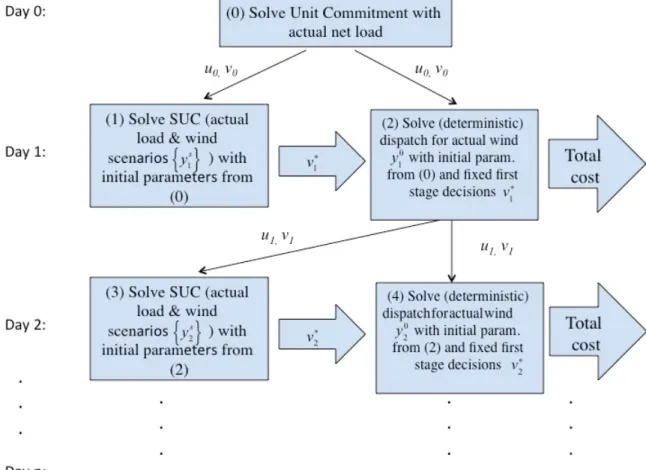
The simulation procedure over a historical time period is depicted in Figure 1:
Fig. 1 SUC and dispatch simulation procedure over a historical time period
We initialized the unit commitment solution procedure using the commitment at the end of the previous day of the historical time period to set the units’ initial on/off states and past durations as well as power generation levels at the beginning of the solution time period. To decide the initial parameters on Day 1 of the historical time period, we solved the deterministic unit commitment and dispatch problem with the observed load and observed wind energy for the previous day, which is represented by Day 0 in Figure 1. Minimum up and down time constraints for the generation units can affect the next day’s initial decisions because if a unit is on (off) at the end of the day, it still must be on (off) the next day until it reaches its minimum up (down) time. Moreover, to satisfy the ramp
13
rate constraints for the first hour of the day, we need the previous day’s power generation amounts for the last hour. To mitigate end-of-horizon effects, we employed a planning horizon of 36 hours, where we repeated the first 12 hours’ net load demand for the last 12 hours. For the first day of the historical period, we solved the SUC problem with probabilistic wind power scenarios 1s
y given the initial parameters from the previous day
and obtained the first stage decision variables, v1. We fixed them to their optimal values
and solved the economic dispatch problem, which is represented by equations (4) and formula (5), with the actual load and observed wind 0
1
y as well as the same initial
parameters obtained from the previous day. Because fixed commitments are applied in the economic dispatch problem, the start-up costs and minimum up and down time constraints need not be considered. Finally, second stage decision variable u1is obtained with actual
net load rather than expectation over scenarios. The total costs and results are recorded and the same steps repeated for the remaining days of the historical time period.
This procedure is repeated using wind power scenarios for each day generated by each of several methods. The hypothesized scenario impacts on cost are as follows: Scenarios that are focused too narrowly (too sharp in the parlance of ensemble forecasts) cause failure to account for the actual risk, and too few low-cost units committed. This may result in starting up additional high cost units or even penalties on load mismatch. If the scenarios are too widely dispersed, the optimization result is too risk averse, and too many units are committed. This may result in excessive no-load cost of committed units. Failure to capture the likelihood of critical events, such as severe down-ramps in wind energy, in the scenarios may likewise result in high dispatch costs.
5. Case study
For our case study, we compiled data to represent a recent year in a down-scaled representation of a region. For statistical assessment we used the whole year’s worth of scenarios, whereas we arbitrarily choose one week from each season to assess the wind power scenarios’ performance according to the SUC simulation results.
5.1. The dataset
To generate wind power scenarios we used the day-ahead hourly wind forecast and observation data from the Bonneville Power Administration (BPA) from 2012/10/01 to 2013/09/31 [45,46]. The days with missing data and/or with wind states considered abnormal were ignored, as documented in detail in [4]. Because only spatially aggregated wind power data are available from BPA, we also aggregated load to a single-bus system, so that transmission constraints were not considered. We obtained the load data from Independent System Operator of New England (NE) [47]. All eight load zones in ISO-NE were treated as a single bus. To focus on the effects of wind power uncertainty we used
14
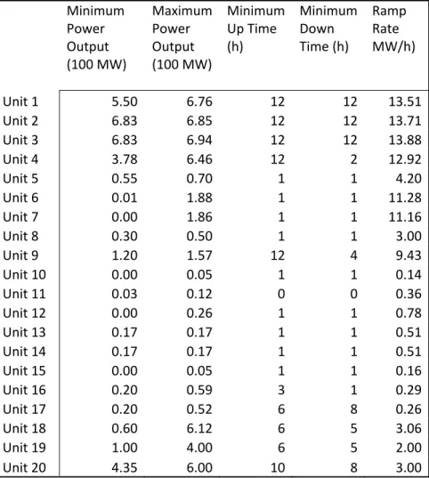
the observed load and generated probabilistic scenarios only for wind power. Thus, the net load scenarios were obtained by subtracting wind power scenarios from the observed load. A representative subset of 20 generators was selected to keep the computation time manageable. Thus, we scaled the net load scenarios (observed load less wind scenarios) and the observed net load by the ratio of the capacity of the selected generators to the total installed capacity. The characteristics of the generators are given in Table 1 and 2. When simulating the SUC procedure we assumed a 20% wind penetration and omitted reserve requirements. We imposed severe penalties in the optimization of $1 million and $10 thousand per kWh as penalty costs for shortage and excess, respectively.
Table 1 Generator physical characteristics
Minimum Power Output (100 MW) Maximum Power Output (100 MW) Minimum Up Time (h) Minimum Down Time (h) Ramp Rate MW/h) Unit 1 5.50 6.76 12 12 13.51 Unit 2 6.83 6.85 12 12 13.71 Unit 3 6.83 6.94 12 12 13.88 Unit 4 3.78 6.46 12 2 12.92 Unit 5 0.55 0.70 1 1 4.20 Unit 6 0.01 1.88 1 1 11.28 Unit 7 0.00 1.86 1 1 11.16 Unit 8 0.30 0.50 1 1 3.00 Unit 9 1.20 1.57 12 4 9.43 Unit 10 0.00 0.05 1 1 0.14 Unit 11 0.03 0.12 0 0 0.36 Unit 12 0.00 0.26 1 1 0.78 Unit 13 0.17 0.17 1 1 0.51 Unit 14 0.17 0.17 1 1 0.51 Unit 15 0.00 0.05 1 1 0.16 Unit 16 0.20 0.59 3 1 0.29 Unit 17 0.20 0.52 6 8 0.26 Unit 18 0.60 6.12 6 5 3.06 Unit 19 1.00 4.00 6 5 2.00 Unit 20 4.35 6.00 10 8 3.00
Table 2 Generator cost characteristics
15 Cold Start Up ($) Medium Start Up ($) Hot Start Up ($) A0 ($/hr) A1 ($/MWhr) A2 ($/MWhr^2) Unit 1 30.79 19.25 19.09 0.00 0.06 0.61 Unit 2 26.90 22.93 18.96 0.00 0.06 0.57 Unit 3 26.90 22.93 18.96 0.00 0.06 0.56 Unit 4 0.00 0.00 0.00 4.96 0.05 0.49 Unit 5 0.85 0.85 0.85 0.00 2.69 26.87 Unit 6 1.01 1.01 1.01 0.00 1.42 14.18 Unit 7 7.22 6.94 6.66 0.00 1.34 13.35 Unit 8 0.00 0.00 0.00 0.00 6.81 68.10 Unit 9 0.00 0.00 0.00 2.25 0.54 5.41 Unit 10 0.00 0.00 0.00 0.00 9.34 93.42 Unit 11 0.00 0.00 0.00 0.00 3.9 38.97 Unit 12 0.00 0.00 0.00 0.00 2.38 23.82 Unit 13 0.00 0.00 0.00 0.00 6.10 60.95 Unit 14 0.00 0.00 0.00 0.00 6.10 60.95 Unit 15 0.00 0.00 0.00 0.00 9.55 95.48 Unit 16 0.00 0.00 0.00 0.00 1.63 16.29 Unit 17 0.00 0.00 0.00 0.00 1.20 11.96 Unit 18 47.36 27.61 4.59 0.00 0.03 0.33 Unit 19 15.97 9.49 3.02 0.00 0.16 1.59 Unit 20 86.55 58.31 30.06 4.38 0.24 2.39
5.2. Wind power scenario generation
Two different methods were used to generate scenarios. The first one is the quantile regression with Gaussian copula approach [26,4]. For this method, we start by estimating a distribution of day-ahead wind power forecast error based on the historical data after the day-ahead wind power forecast is obtained. For each hour of the day ahead, a quantile regression model estimates the 0.05, 0.10, …, 0.95 quantiles of forecast error based on forecasted wind power generation. Then, by linearly interpolating the quantiles with hypothetical minimum and maximum forecast error, we estimate the distribution of forecast error for each hour. The Gaussian copula method transforms the 24 hourly forecast error distributions into a multivariate Gaussian distribution with covariance of forecast errors of different hours. Thus, we can easily generate forecast error scenarios by projecting Monte Carlo samples from the multivariate Gaussian distribution onto 24 forecast error distributions. Finally the forecast error scenarios are added to the day-ahead forecast to generate day-ahead wind power scenarios (labeled as QR) [4]. Moreover, we re-modeled the tails by adding another quantile (0.01 and 0.99) to linearly interpolate and truncating
16
the remaining tails (<0.01, >0.99). This variant results in slightly smoother scenarios (labeled as QRnew).
The second scenario generation method is an epi-spline approximation approach [48], and two different variants are generated with cutting probabilities (0, 0.1, 0.9, 1) and (0, 0.33, 0.66 1) [4]. For this method, first error distributions are approximated using exponential epi-splines. Hours within the day are partitioned into intervals by day-part separators (dps; i.e., specific hours of the day). A set of cutting probabilities of error distributions is predefined. Scenarios are generated by the following steps [49]:
1. Cluster forecasts in the training set according to patterns of their left-hand, right-hand and pointwise derivatives at dps hours.
2. Within each cluster, approximate the log error density for each hour with an epi-spline as described in [48]. Numerically integrate to obtain cdfs of the error distributions. 3. Given a forecast of hourly wind power values, identify the cluster to which the forecast belongs at each dps. Compute “skeleton points” for each dps as conditional expected values between the quantiles corresponding to the predefined cutting probabilities.
4. Combine the skeleton points throughout the day.
We use the labels EPI(0.1, 0.9) and EPI(0.33, 0.66) to denote the epi spline scenarios obtained with different cutting points. Each wind power scenario set has 27 scenarios.
5.3. Results and Discussion
The SUC and dispatch problems were solved in their extensive forms by PySP [50] using CPLEX as the MIP solver over the selected historical time periods. Results of the historical time period simulations and statistical metrics are presented in this section. In the plots , we use date IDs given in Table 3.
Table 3 Date IDs and date ranges of the 4 historical time periods used for the SUC simulations
Time period Date range Date ID (i=1,…,7) 1 2012/10/17 – 2012/10/23 1_i 2 2013/01/01 – 2013/01/07 2_i 3 2013/04/14 – 2013/04/20 3_i 4 2013/07/07 – 2013/07/13 4_i
17
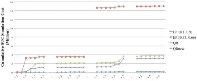
Figure 2 plots the cumulative costs of our SUC and dispatch simulation for wind power scenarios generated by EPI(0.1, 0.9), EPI(0.33, 0.66), QR and QRnew. As can be seen, EPI(0.1, 0.9) performs the best, whereas EPI(0.33, 0.66) is the worst. We observe a slight improvement in QRnew compared to QR.
Fig. 2 Cumulative SUC and dispatch costs over 4 historical time periods
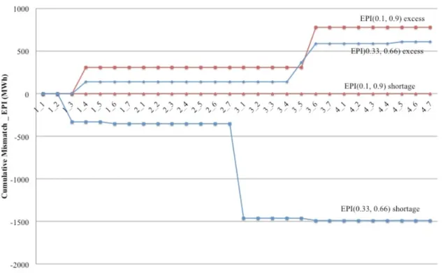
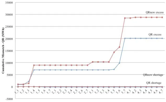
Figures 3 and 4 show the cumulative deviations from optimal generation levels in megawatt hours incurred by epi-spline and quantile regression scenarios over 4 historical time periods, respectively.
Tables 4 and 5 show the dates when there occur positive and/or negative mismatch by epi-spline and quantile regression scenarios, respectively. The excess and shortage amounts relative to the optimal generation levels are expressed as percentages.
18
Fig. 3 Cumulative deviations from optimal generation level occurred by epi-spline
scenarios over 4 historical time periods
Table 4 Percentages of deviations from the optimal generation levels by Epi spline scenarios.
EPI(0.1, 0.9) EPI(0.33, 0.66)
Date excess(%) shortage(%) excess(%) shortage(%)
2012/10/19 0 0 0 0.674 2012/10/20 3.221 0 0.785 0 2012/10/22 0 0 0 0.031 2013/4/14 0 0.005 0 3.121 2013/4/18 0 0 0.779 0 2013/4/19 1.756 0 0.098 0.848 2013/4/20 0.096 0 0 0 2013/7/11 0 0 0.295 0
19
Fig. 4 Cumulative deviations from optimal generation levels occurred by quantile
regression scenarios over 4 planning historical time periods
Table 5: Percentages of deviations from the optimal generation levels by quantile regression scenarios.
QR QRnew
Date excess(%) shortage(%) excess(%) shortage(%)
2012/10/17 1.489 0 1.790 0 2012/10/19 2.729 0 0.770 0 2012/10/20 26.880 0 42.750 0 2012/10/21 0 1.511 0 0 2012/10/22 0 0.045 0 0.310 2013/4/14 0 0 3.990 0
20 2013/4/15 0 0.012 0 0 2013/4/18 0.604 0 13.660 0 2013/4/19 9.909 0.044 8.430 0 2013/4/20 245 0 288 0 2013/7/8 0 0.011 0.330 0
Figure 5 shows the MTD rank histograms of wind power scenarios after de-biasing and scaling. To quantify the uniformity of the resulting MTD rank histograms we use the Cramér-von Mises goodness of fit statistic because it is sensitive to skewed rank histograms. According to the Cramèr‐von Mises test, where the critical value is 0.33, we reject the null hypothesis of uniformity for all four rank histograms at the 1% significance level.
21
Fig. 5 Mass transportation distance rank histograms for scenarios EPI(0.1, 0.9),
EPI(0.33, 0.66), QR, and QRnew
The MTD rank histogram is useful for checking the statistical reliability of scenarios according to their bias, variability, and autocorrelation, as mentioned earlier. Apparently in Figure 5 the smallest rank is over-populated in the histogram of EPI(0.33, 0.66), which indicates under-dispersion. This scenario set prevents the optimization from accounting for the actual risk due to the inherent uncertainty in wind. The high difference in SUC and dispatch cost in Figure 2 is due to the high penalties assigned to positive mismatch (shortage) in load and startup costs for additional high-cost units. The largest proportion of the cost is due to the unsatisfied demand, which may happen when the observed wind power availability is lower than all of the wind power scenario trajectories at some time period.
The cumulative deviations from optimal generation levels and percentages of deviations incurred by epi-spline scenarios are represented in Figure 3 and Table 4, respectively. EPI(0.33, 0.66) results in higher and more frequent shortage than the other scenario sets. This is a result of under-dispersion as indicated by the overpopulation of smallest ranks in MTD rank histogram in Figure 5. We conjecture that using EPI(0.33, 0.66) scenarios will result in the highest cost over the whole year. As explained and shown by simulation studies in [4], heterogeneous autocorrelation levels in scenarios cause rank histograms to be hill-shaped, as observed in the histogram for QR in Figure 5. This is one result of having both very wildly varying and smooth scenarios. Optimization is risk averse with those scenarios and as a result too many low-cost units may be committed, and excessive no-load costs of committed units occur. Moreover, too many committed units will cause penalty costs due to excess because of the minimum power generation limit constraints of the units as seen in Figure 4 and Table 5. Thus, the penalty costs for excess are higher and occur more frequently for the quantile regression scenarios than the epi-spline scenarios (Tables 4 and 5). Moreover, even if we ignore all penalty costs due to the mismatch in load, we still observe that quantile regression scenarios result in higher costs than do the epi-spline scenarios. After better modeling the tails in the quantile regression scenario generation method, we obtained slightly smoothed scenarios. This is indicated by a flatter histogram as seen in Figure 5 (QRnew). Eliminating very wild scenarios results in slightly lower costs in SUC in Figure 2. However, we still observe some penalty costs due to shortage in demand in all of the variants of the QR scenarios (Figure 3 and Table 5). The shortage is not because of the under-dispersion as in EPI(0.33, 0.66), but because of the sampling behavior.
As explained and shown with the simulation studies in [4], under-dispersion, over-dispersion, and differences in autocorrelation levels affect the skewness of the rank histogram, whereas heterogeneous autocorrelation levels in scenario set overpopulate the middle of the rank histogram. Moreover, some combinations of all these statistics may
22
result in a misleadingly flat histogram, which is a limitation of both the MST and MTD rank histograms. It would not be valid to assert that the wind power scenario set with flattest MTD rank histogram would perform the best in a SUC and dispatch solution procedure over a historical time period. However, we can eliminate the scenario sets having right-skewed and hill-shaped rank histograms because the majority of the costs occur because of under-dispersion (which result in penalties due to positive mismatch in load) and heterogeneous autocorrelation levels in the scenario set (which result in committing too many units, excessive no-load costs and penalties due to negative mismatch in load). In our case study, we can choose EPI(0.1, 0.9) over EPI(0.33, 0.66) and QRnew over QR. The MTD rank histogram seems to be better able to distinguish among the variants of each scenario generation methods than across the methods.
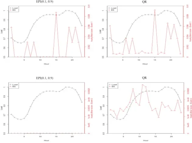
We assessed the scenarios according to the RampDown event with 2 different sets of parameters. The average daily Brier scores are represented in Table 6 and the plots in Figure 6 show the average hourly Brier scores and average hourly loads.
Table 6. Average daily Brier scores for RampDown event with two different parameters for scenarios EPI(0.1, 0.9), EPI(0.33, 0.66), QR, and QRnew.
Table 6 shows the average daily Brier scores for RampDown events with two different parameters. One limitation of Brier score to evaluate wind power scenarios is that it gives very low scores when the scenario sets are too sharp. Since the under-dispersed EPI(0.33, 0.66) scenarios are too sharp, they result in low scores whereas their costs are too high in SUC. However, if the scenario set is not under-dispersed, the Brier scores of RampDown events are very successful to catch the differences over the scenarios. As can be seen from Table 6, QRhas the highest Brier score whereas EPI(0.1, 0.9) has the lowest.
Events EPI(0.1, 0.9) EPI(0.33, 0.66) QR QRnew 1-RampDown(=1, ξ=0.2) 0.0015 0.0015 0.0023 0.0018 2-RampDown(=1, ξ=0.4) 0.0000 0.0000 0.0002 3.3e-06
23
Fig. 6 Hourly average load and average hourly Brier scores for Event 1 and 2
Figure 6 shows hourly average load and average hourly Brier scores according to the events shown in Table 6 for the wind power scenario sets that have the highest and lowest average daily Brier scores. The load ramps up after hour 9, and the peak load occurs between hours 12 and 21. Thus, the differences among Brier scores of wind power scenarios during those hours are more critical. If the wind power scenarios do not successfully reflect the likelihood of the RampDown event in that time range, expensive peaking generators would be required to satisfy the unexpectedly high net load.
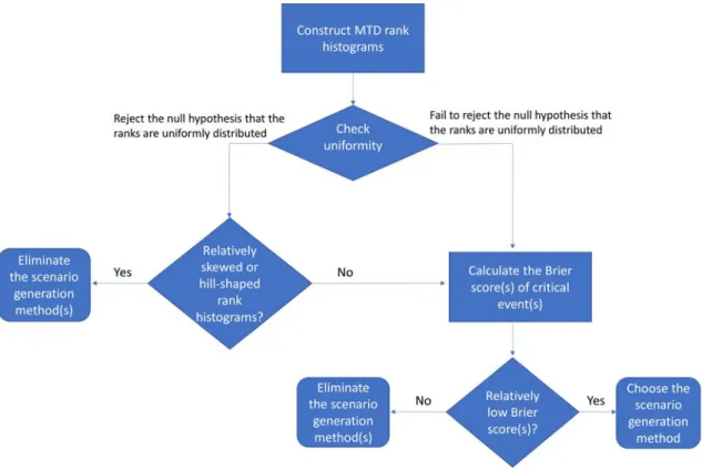
To summarize, we would expect a successful collection of wind power scenario sets to first be reliable, which means a good level of correspondence between scenario distribution and observation distribution according to their autocorrelation and variability and, second, to represent the critical events such as RampDown and RampUp with some specific parameters for our SUC and dispatch problem. We recommend to first use the MTD rank histograms to eliminate the scenario generation methods that produced underdispersed scenarios (right-skewed rank histogram) and/or scenarios with inaccurate autocorrelation levels (hill-shaped rank histogram). Then compare the remaining scenario collections according to the Brier scores of the RampDown event. This process is depicted in Figure
24
7, where the word “relatively” refers to comparisons among the collections of scenario sets produced by competing scenario generation methods.
Fig. 7 Process for selecting from among alternative scenario generation methods
5.4.Daily comparisons
In this section, for some specific days we display plots of wind power scenarios generated by two variants of each methods and represent daily SUC and dispatch costs by comparing some cost components to give additional insight.
Figures 8 and 9 show the wind power scenarios generated by epi-spline approximation on the left and quantile regression with Gaussian copula approach on the right. Wind energy is scaled according to the capacity.
25
Fig. 8 Wind power scenarios generated for day 2012/10/19. (a) EPI(0.1, 0.9), (b)
EPI(0.33, 0.66), (c) QR, (d) QRnew
For day 2012/10/19 the SUC costs resulting from using the different wind power scenarios are ordered as EPI(0.33,0.66)> QR> QRnew> EPI(0.1,0.9). The majority of the costs occur because of the penalties for all the scenario sets except EPI (0.1, 0.9). However, EPI(0.33, 0.66) has the highest penalties. No-load costs for EPI scenarios are lower than QR scenarios.
26
Fig. 9 Wind power scenarios generated for day 2013/04/19. (a) EPI(0.1, 0.9), (b)
EPI(0.33, 0.66), (c) QR, (d) QRnew
For day 2013/04/19, all of the scenario sets have penalty due to excess, and the amount of excess is ordered as QR> QRnew> EPI(0.1, 0.9)> EPI(0.33, 0.66). Only EPI(0.33, 0.66) and QR caused shortage penalties and the shortage amount is higher for EPI(0.33, 0.66).
27
Fig. 10 Wind power scenarios and net load scenarios for day 2013/04/14. (a) EPI(0.1,
0.9), (b) EPI(0.33, 0.66), (c) Net load scenarios for EPI(0.1, 0.9), (d) Net load scenarios for EPI(.33, 0.66)
Figure 10 shows the plots of wind scenarios on the left-hand side and net load (observed load – wind scenario) scenarios after scaling according to the generator capacity and adjusting according to the 20% wind penetration on the right. On day 2013/04/14, no negative mismatch occurred for both of the epi spline wind scenario sets. However, there was positive mismatch for both, which corresponded to 0.005% and 3.121% deviation from the optimal generation level for EPI(0.1, 0.9) and EPI(0.33, 0.66), respectively.
6. Conclusions
A stochastic unit commitment formulation for uncertain wind power can achieve cost savings but the computation time increases with the dimension of the deterministic optimization and the number of scenarios. To facilitate a comparison among scenario generation methods using observations over a long historical time period, we employ two statistical metrics: mass transportation distance rank histogram and event based verification. Our case study indicates that these statistical tools can predict the performance
28
of the resulting unit commitment schedules when the committed units are dispatched to meet the observed demand. Two different scenario generation methods and their variants are compared according to their performance in a simulation of the SUC procedure. Using the mass transportation distance rank histogram we can eliminate the scenario generation methods that might lead to either high no-load costs or high penalty costs due to shortage or excess. Then, after defining critical event(s) for the problem we compare the scenario collections produced by the remaining generation methods according to their Brier scores. Both metrics have limitations. For some specific combinations of over-dispersion and weak correlation, the MTD rank histogram appears deceptively flat. Moreover, Brier scores may be very low for under-dispersed and/or sharp scenario sets. According to the results of the case study, we can conclude that, of the wind power scenario generation methods and variants tested, the epi-spline approximation approach with cutting probabilities (0, 0.1, 0.9, 1) performs the best in the SUC problem, as could be predicted by its flat MTD rank histogram and low Brier scores for ramp-down events.
In future work, this study could be extended to a multi-area setting, in which transmission constraints would also be included in the SUC formulation. Both scenario generation methods tested here use day-ahead forecasts of wind power time series. Thus, testing the resulting collections of scenario sets in the historical simulation would require a data set of not only observations but also historical day-ahead multi-area forecasts of wind power, which we have thus far not been able to obtain. The MTD rank histogram would easily accommodate the increased dimensionality of each scenario, but larger scenario sets and/or longer historical time periods might be required to distinguish among scenario generation methods. Developing appropriate event descriptions on which to compute Brier scores would be a more intricate task in this setting.
REFERENCES
1. Zheng, Q.P.P., Wang, J.H., Liu, A.L.: Stochastic Optimization for Unit Commitment‐A Review. IEEE T Power Syst 30(4), 1913‐1924 (2015).
2. Gneiting, T., Balabdaoui, F., Raftery, A.E.: Probabilistic forecasts, calibration and sharpness. J Roy Stat Soc B 69, 243‐268 (2007).
3. Hsu, W.R., Murphy, A.H.: The Attributes Diagram ‐ a Geometrical Framework for Assessing the Quality of Probability Forecasts. Int J Forecasting 2(3), 285‐293 (1986). doi:Doi 10.1016/0169‐2070(86)90048‐8
4. Sari, D., Lee, Y., Ryan, S., Woodruff, D.: Statistical metrics for assessing the quality of wind power scenarios for stochastic unit commitment. Wind Energy 19(5), 873‐893 (2016).
5. Ortega‐Vazquez, M.A., Kirschen, D.S.: Assessing the Impact of Wind Power Generation on Operating Costs. IEEE T Smart Grid 1(3), 295‐301 (2010).
29
6. Ummels, B.C., Gibescu, M., Pelgrum, E., Kling, W.L., Brand, A.J.: Impacts of wind power on thermal generation unit commitment and dispatch. IEEE T Energy Conver 22(1), 44‐51 (2007).
7. Tuohy, A., Meibom, P., Denny, E., O'Malley, M.: Unit Commitment for Systems With Significant Wind Penetration. IEEE T Power Syst 24(2), 592‐601 (2009). 8. Yang, Y.C., Wang, J.H., Guan, X.H., Zhai, Q.Z.: Subhourly unit commitment with
feasible energy delivery constraints. Appl Energ 96, 245‐252 (2012).
9. Osorio, G.J., Lujano‐Rojas, J.M., Matias, J.C.O., Catalao, J.P.S.: A probabilistic approach to solve the economic dispatch problem with intermittent renewable energy sources. Energy 82, 949‐959 (2015).
10. Ortega‐Vazquez, M.A., Kirschen, D.S.: Optimizing the spinning reserve requirements using a cost/benefit analysis. IEEE T Power Syst 22(1), 24‐33 (2007).
11. Ela, E., O'Malley, M.: Studying the Variability and Uncertainty Impacts of Variable Generation at Multiple Timescales. IEEE T Power Syst 27(3), 1324‐1333 (2012).
12. Zhou, Z., Botterud, A., Wang, J., Bessa, R.J., Keko, H., Sumaili, J., Miranda, V.: Application of probabilistic wind power forecasting in electricity markets. Wind Energy 16(3), 321‐338 (2013).
13. Takriti, S., Birge, J.R., Long, E.: A stochastic model for the unit commitment problem. IEEE T Power Syst 11(3), 1497‐1506 (1996).
14. Bakirtzis, E.A., Biskas, P.N., Labridis, D.P., Bakirtzis, A.G.: Multiple Time Resolution Unit Commitment for Short‐Term Operations Scheduling Under High Renewable Penetration. IEEE T Power Syst 29(1), 149‐159 (2014).
15. Papavasiliou, A., Oren, S.S.: Multiarea Stochastic Unit Commitment for High Wind Penetration in a Transmission Constrained Network. Oper Res 61(3), 578‐592 (2013).
16. Wu, H.Y., Shahidehpour, M.: Stochastic SCUC Solution With Variable Wind Energy Using Constrained Ordinal Optimization. IEEE T Sustain Energ 5(2), 379‐388 (2014).
17. Madaeni, S.H., Sioshansi, R.: The impacts of stochastic programming and demand response on wind integration. Energy Systems 4(2), 109‐124 (2013). doi:10.1007/s12667‐012‐0068‐7
18. Bouffard, F., Galiana, F.D.: Stochastic security for operations planning with significant wind power generation. IEEE T Power Syst 23(2), 306‐316 (2008). 19. Ruiz, P.A., Philbrick, C.R., Zak, E., Cheung, K.W., Sauer, P.W.: Uncertainty
Management in the Unit Commitment Problem. IEEE T Power Syst 24(2), 642‐ 651 (2009).
20. Wang, J.D., Wang, J.H., Liu, C., Ruiz, J.P.: Stochastic unit commitment with sub‐ hourly dispatch constraints. Appl Energ 105, 418‐422 (2013).
21. Quan, H., Srinivasan, D., Khambadkone, A.M., Khosravi, A.: A computational framework for uncertainty integration in stochastic unit commitment with intermittent renewable energy sources. Appl Energ 152, 71‐82 (2015). 22. Ela, E., Milligan, M., O'Malley, M.: A Flexible Power System Operations Simulation
30
23. Papavasiliou, A., Oren, S.S., O'Neill, R.P.: Reserve Requirements for Wind Power Integration: A Scenario‐Based Stochastic Programming Framework. IEEE T Power Syst 26(4), 2197‐2206 (2011).
24. Wang, J., Botterud, A., Bessa, R., Keko, H., Carvalho, L., Issicaba, D., Sumaili, J., Miranda, V.: Wind power forecasting uncertainty and unit commitment. Appl Energ 88(11), 4014‐4023 (2011).
25. Morales, J.M., Minguez, R., Conejo, A.J.: A methodology to generate statistically dependent wind speed scenarios. Appl Energ 87(3), 843‐855 (2010).
26. Pinson, P., Madsen, H., Nielsen, H.A., Papaefthymiou, G., Klockl, B.: From Probabilistic Forecasts to Statistical Scenarios of Short‐term Wind Power Production. Wind Energy 12(1), 51‐62 (2009).
27. Pinson, P., Girard, R.: Evaluating the quality of scenarios of short‐term wind power generation. Appl Energ 96, 12‐20 (2012).
28. Gneiting, T., Stanberry, L.I., Grimit, E.P., Held, L., Johnson, N.A.: Assessing probabilistic forecasts of multivariate quantities, with an application to ensemble predictions of surface winds. Test 17(2), 211‐235 (2008).
29. Wilks, D.S.: The minimum spanning tree histogram as a verification tool for multidimensional ensemble forecasts. Mon Weather Rev 132(6), 1329‐1340 (2004).
30. Gombos, D., Hansen, J.A., Du, J., McQueen, J.: Theory and applications of the minimum spanning tree rank histogram. Mon Weather Rev 135(4), 1490‐ 1505 (2007).
31. Brier, G.W.: Verification of Forecasts Expressed in Terms of Probability. Mon Weather Rev 78(1), 1‐3 (1950). doi:10.1175/1520‐ 0493(1950)078<0001:VOFEIT>2.0.CO;2
32. Bruninx, K., Dvorkin, Y., Delarue, E., Pandzic, H., D'haeseleer, W., Kirschen, D.S.: Coupling Pumped Hydro Energy Storage With Unit Commitment. IEEE T Sustain Energ 7(2), 786‐796 (2016).
33. Siface, D., Vespucci, M.T., Gelmini, A.: Solution of the mixed integer large scale unit commitment problem by means of a continuous Stochastic linear programming model. Energy Systems 5(2), 269‐284 (2014). doi:10.1007/s12667‐013‐0107‐z
34. Bruninx, K., Bergh, K.V.d., Delarue, E., haeseleer, W.D.: Optimization and Allocation of Spinning Reserves in a Low‐Carbon Framework. IEEE T Power Syst 31(2), 872‐882 (2016). doi:10.1109/TPWRS.2015.2430282
35. Shukla, A., Singh, S.N.: Clustering based unit commitment with wind power uncertainty. Energ Convers Manage 111, 89‐102 (2016).
36. Feng, Y., Ryan, S.M.: Solution sensitivity‐based scenario reduction for stochastic unit commitment. Computational Management Science 13(1), 29‐62 (2016). doi:10.1007/s10287‐014‐0220‐z
37. Ji, B., Yuan, X.H., Chen, Z.H., Tian, H.: Improved gravitational search algorithm for unit commitment considering uncertainty of wind power. Energy 67, 52‐62 (2014).
38. Nasri, A., Kazempour, S.J., Conejo, A.J., Ghandhari, M.: Network‐Constrained AC Unit Commitment Under Uncertainty: A Benders' Decomposition Approach. IEEE T Power Syst 31(1), 412‐422 (2016).
31
39. Cheung, K., Gade, D., Silva‐Monroy, C., Ryan, S.M., Watson, J.P., Wets, R.J.B., Woodruff, D.L.: Toward scalable stochastic unit commitment Part 2: solver configuration and performance assessment. Energy Syst 6(3), 417‐438 (2015). doi:10.1007/s12667‐015‐0148‐6
40. Thorarinsdottir, T.L., Scheuerer, M., Heinz, C.: Assessing the Calibration of High‐ Dimensional Ensemble Forecasts Using Rank Histograms. Journal of Computational and Graphical Statistics 25(1), 105‐122 (2016). doi:10.1080/10618600.2014.977447
41. Dupacova, J., Gröwe‐Kuska, N., Römisch, W.: Scenario reduction in stochastic programming: An approach using probability metrics. Math Program 95(3), 493‐511 (2003). doi:10.1007/s10107‐002‐0331‐0
42. Rachev, S.T.: Probability Metrics and the Stability of Stochastic Models. Wiley, New York (1991)
43. Rachev, S.T., Rüschendorf, L.: Mass Transportation Problems. Probability and Its Applications. Springer‐Verlag Berlin (1998)
44. Feng, Y.H., Rios, I., Ryan, S.M., Spurkel, K., Watson, J.P., Wets, R.J.B., Woodruff, D.L.: Toward scalable stochastic unit commitment. Part 1: load scenario generation. Energy Syst 6(3), 309‐329 (2015). doi:10.1007/s12667‐015‐0146‐8
45. . http://transmission.bpa.gov/Business/Operations/Wind/default.aspx.
46. . http://www.bpa.gov/Projects/Initiatives/Wind/Pages/Wind‐Power‐ Forecasting‐Data.aspx. 2016
47. . http://www.iso‐ne.com/isoexpress/web/reports/pricing/‐/tree/zone‐info. 48. Royset JO, W.R.‐B.: Nonparametric density estimation via exponential epi‐eplines:
Fusion of soft and hard information. https://www.math.ucdavis.edu/~rjbw/mypage/Statistics_files/RstW13_xsp l.pdf (2013).
49. Rios, I., Wets, R.J.‐B., Woodruff, D.L.: Multi‐period forecasting and scenario generation with limited data. Computational Management Science 12(2), 267‐ 295 (2015). doi:10.1007/s10287‐015‐0230‐5