SHORT TERM LOAD FORECASTING USING A NEURAL NETWORK BASED TIME SERIES APPROACH
By
SUCI DWIJAYANTI
Bachelor of Science in Electrical Engineering Sriwijaya University
Palembang, Indonesia 2006
Submitted to the Faculty of the Graduate College of the Oklahoma State University
in partial fulfillment of the requirements for
the Degree of MASTER OF SCIENCE
SHORT TERM LOAD FORECASTING USING A NEURAL NETWORK BASED TIME SERIES APPROACH
Thesis Approved:
Dr. Martin Hagan Thesis Advisor Dr. Carl Latino
ACKNOWLEDGMENTS
It gives me great pleasure in expressing my gratitude to all those people who have sup-ported me and had their contributions in making this thesis possible. First and foremost, I must acknowledge and thank The Almighty Allah SWT for blessing, protecting and guid-ing me throughout this period. I could never have accomplished this without the faith I have in the Almighty.
I am indebted and would like to express my deepest gratitude to my advisor, Dr. Martin Hagan, for his excellent guidance, caring, patience, and providing me with an excellent atmosphere for doing research. I would also like to thank Dr. Carl Latino and Dr. R.G. Ramakumar for serving on my committee, for their support and advisement. While doing this thesis, I would never have been able to finish it without help from friends and support from my family. I would like to thank my friend Leni for her help in obtaining the data from PT. PLN Batam Indonesia and all of my friends for their help during the time I am here. Last and most importantly, I would also like to thank my parents, Rahman HS and Suwasti, my sister, Agustin Darmayanti, and brothers, Ridho Akbar and Norman Wibowo, for their endless love, support and encouragement.
Name: SUCI DWIJAYANTI Date of Degree: May, 2013
Title of Study: SHORT TERM LOAD FORECASTING USING A NEURAL NETWORK BASED TIME SERIES APPROACH
Major Field: Electrical Engineering
Short term load forecasting (STLF) is important, since it is used to maintain optimal per-formance in the day-to-day operation of electric utility systems. The autoregressive inte-grated moving average (ARIMA) model is a linear prediction method that has been used for STLF. However, it has a weakness. It assumes a linear relationship between current and future values of load and a linear relationship between weather variables and load con-sumption. Neural networks have the ability to model complex and nonlinear relationships. Therefore, they can be used as a robust method for nonlinear prediction, and they can be trained with historical hourly load data. The purpose of this work is to describe how neural networks can transform linear ARIMA models to create short term load prediction tools. This thesis introduces a new neural network architecture - the periodic nonlinear ARIMA (PNARIMA) model. In this work, first, we make linear predictions of the daily load using ARIMA models. Then we test the PNARIMA predictor. The predictors are tested using load data (from May 2009 - April 2011) from Batam, Indonesia. The results show that the PNARIMA predictor is better than the ARIMA predictor for all testing periods. This demonstrates that there are nonlinear characteristics of the load that cannot be captured by ARIMA models. In addition, we demonstrate that a single model can provide accu-rate predictions throughout the year, demonstrating that load characteristics do not change substantially between the wet and dry seasons of the tropical climate of Batam, Indonesia.
TABLE OF CONTENTS
Chapter Page
1 INTRODUCTION 1
2 SHORT TERM LOAD FORECASTING 5
2.1 Overview of Load Forecasting . . . 5
2.2 The importance for short term load forecasting . . . 8
2.3 Short term load forecasting methods . . . 11
2.3.1 Conventional or classical approaches . . . 11
2.3.2 Computational intelligence based techniques . . . 15
3 ARIMA MODELING 20 3.1 Linear time series Overview . . . 20
3.1.1 Stationary stochastic processes . . . 20
3.1.2 Autocovariance and autocorrelation function . . . 21
3.1.3 Differencing . . . 22
3.1.4 White noise . . . 23
3.2 AR, MA, ARMA and ARIMA Models . . . 23
3.3 Time series models for prediction . . . 27
3.3.1 Model identification . . . 27
3.3.2 Parameter estimation . . . 33
3.3.3 Diagnostic testing . . . 34
4 NEURAL NETWORKS FOR FORECASTING 38
4.1 Neural Networks Overview . . . 38
4.2 Designing neural networks for forecasting . . . 44
4.2.1 Data Collection and pre-processing . . . 45
4.2.2 Selecting the network type and architecture . . . 46
4.2.3 Selecting training algorithm . . . 47
4.2.4 Analyzing network performance . . . 52
5 RESULTS 54 5.1 Data Description . . . 54
5.2 Fitting the ARIMA model . . . 59
5.2.1 Preliminary model structure determination . . . 60
5.2.2 Parameter estimation and model validation . . . 64
5.3 Fitting the neural network model . . . 68
5.3.1 Preliminary structure determination . . . 68
5.3.2 Form of neural network prediction . . . 71
5.3.3 Fitting and validation of the neural network model . . . 75
5.4 Comparison of ARIMA and neural network models on test data . . . 77
6 CONCLUSIONS 80
REFERENCES 83
LIST OF TABLES
Table Page
3.1 Behaviour of Theoretical ACF and PACF for Stationary Process . . . 30
3.2 GPAC Array . . . 32
3.3 GPAC Array for An ARMA(p, q)Process . . . 33
5.1 Classification and Composition of Consumers . . . 55
5.2 Training and Testing Periods . . . 58
5.3 Confidence Intervals for Final ARIMA Model Training Data August to Oc-tober 2009 . . . 64
5.4 ARIMA Models . . . 67
5.5 Seasonal ARIMA Performance for Training data . . . 68
5.6 PNARIMA Performance for Training data . . . 77
LIST OF FIGURES
Figure Page
2.1 A Typical Configuration of An Electric Power System . . . 6
2.2 An Input-Output Configuration of A STLF System and Its Major Uses . . . 10
3.1 System Identification Steps . . . 27
3.2 ACF and PACF ofzt = 0.5zt−1 +et . . . 29
3.3 ACF and PACF ofzt =et+ 0.8et−1 . . . 30
4.1 General Neuron . . . 39
4.2 Layer ofSNeurons . . . 39
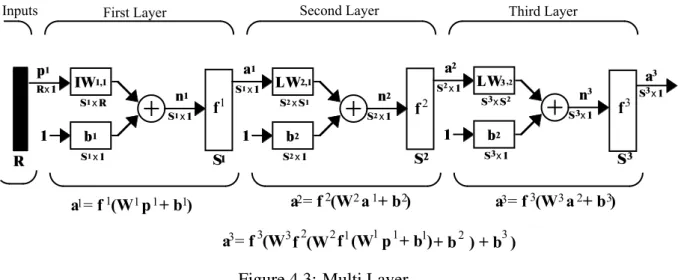
4.3 Multi Layer . . . 40
4.4 Tapped Delay Line . . . 40
4.5 NARX Neural Network . . . 41
4.6 NARX Neural Network Architecture . . . 42
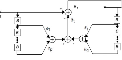
4.7 ARMA Model . . . 42
4.8 Abbreviated Notation of the ARMA Model . . . 43
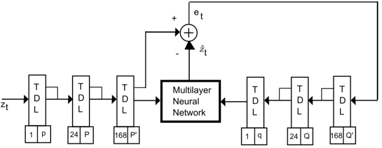
4.9 Nonlinear ARMA (NARMA) Predictor Model Using a Neural Network . . 43
4.10 Periodic NARIMA (PNARIMA) Model . . . 44
4.11 Flowchart of Neural Network Training Process . . . 44
4.12 Neural Networks . . . 48
4.13 Levenberg-Marquardt Flowchart . . . 49
5.1 Hourly Electric Load Consumption for August 3 - 9, 2009 . . . 56
5.3 Relationship Between Temperature and Daily Peak Electric Load
Con-sumption for August, 2009 . . . 57
5.4 ACF and PACF from Original Load August to October, 2009 . . . 60
5.5 ACF Differenced of Load August to October, 2009 . . . 61
5.6 ACF and PACF Load August - October 2009 Difference∇1∇24 . . . 62
5.7 ACF and PACF Residual for Tentative Model . . . 63
5.8 ACF and PACF Residual for Final Model . . . 65
5.9 ARIMA Prediction for One Week in August - October, 2009 . . . 66
5.10 PNARIMA Architecture for Prediction . . . 70
5.11 ACF and PACF Residual for PNARIMA Neural Network . . . 75
5.12 PNARIMA Prediction During a Typical Week During August - October, 2009 . . . 76
5.13 PNARIMA and ARIMA Predictions of Testing Data from The Period from August to October, 2010 . . . 78
LIST OF ABBREVIATIONS AND SYMBOLS
List of Abbreviations
ACF Autocorrelation function PACF Partial autocorrelation function GPAC Generalized partial autocorrelation STLF Short term load forecasting
MTLF Mid term load forecasting LTLF Long term load forecasting ARMA Autoregressive moving average
ARIMA Autoregressive integrated moving average
ARMAX Autoregressive moving average with exogenous input NARIMA Nonlinear autoregressive integrated moving average
PNARIMA Periodic nonlinear autoregressive integrated moving average NARX Nonlinear autoregressive with exogenous input
TDL Tapped delay line RMSE Root mean square error MAE Mean absolute error
List of Symbols
zt Power load of timet
ˆ
zt Predictions of power loadzt
Bnzt Backward shift operatorzt−n ∇d Difference operator(1−B)d
ϕp, θq The autoregressive and moving average parameters
et Error (difference between actual and predicted value)
wt The differenced load at timet
ˆ
wt Predictions of the differenced loadwt
pl(t) Theithinput vector to the network at timet nm(t) The net input for layerm
fm(.) The transfer function for layerm am(t) The output for layerm
IWm,l The input weight between inputland layerm LWm,l The layer weight between layerland layerm bm The bias vector for layerm
DLm,l The set of delays in the tapped delay line between Layerl and Layerm
DIm,l The set of delays in the tapped delay line between Inputland Layerm
Sk Number of neurons in layerk
R Dimension of input vector
||w|| Norm
Wk(t) Weight matrix
CHAPTER 1
INTRODUCTION
Load forecasting plays an important role as a central and integral process in the planning and operation of electric utilities. If the load forecasting is accurate, there will be a great potential savings in the control operations and decision making, such as dispatch, unit com-mitment, fuel allocation, power system security assessment, and off-line analysis. Errors in forecasting the electric load demand will increase operating costs. Bunn and Farmer [1] pointed out that in the UK, a 1% increase in forecasting error implied a£10 million increase in operating costs. If the predicted electric load is higher than the actual demand, the oper-ating cost will increase significantly, and it wastes scarce resources. On the other hand, if the predicted electric load is less than the actual demand, it can cause brownouts and black-outs, which can be costly, especially to large industrial customers. In addition, reliable load forecasting can reduce energy consumption and decrease environmental pollution.
In general, based on the time horizon, electric load forecasting can be organized into three categories: short term, mid term and long term. In this work, we will focus on short term load forecasting (STLF). STLF refers to the prediction of loads for time leads from one hour up to one week ahead. Mandal et.al [2] explained that STLF is an important tool in day to day operation and planning activities of the utility system, such as energy transactions, unit commitment, security analysis, economic dispatch, fuel scheduling and unit maintenance.
STLF is a very complex process, because there are many factors that influence it, such as economic conditions, time, day, season, weather and random effects. Electric load de-mand itself is a function of weather variables, human social activities and industrial
activi-ties. Hipert et.al [3] explain that short term load forecasting becomes complicated because the load at a given hour depends not only on the load of the previous hour but also the load at the same hour on previous days, and the load at the same hour on the day with the same denomination in the previous week. In addition, the predictor needs to model the relation between the load and other variables, such as weather, holiday activities, etc.
During the last few decades, various methods for STLF have been proposed and imple-mented. These methods can be classified into two main types; traditional or conventional and computational intelligence approaches. Time series models, regression models and the Kalman filter are some of the conventional methods. Expert system models, pattern recog-nition models and neural network models are some of the computational intelligence based techniques. Hagan and Klein [4] were the first to use the periodic ARIMA model of Box and Jenkins for STLF. This is a univariate time series model, in which the load is mod-eled as a function of its past observed values, with daily and weekly cycles accounted for. Papalexopoulos and Hesterberg [5] used the regression model for STLF. The disadvantage of the regression model is that complex modeling techniques and heavy computational ef-forts are required to produce reasonably accurate results [6]. Other time series approaches are multiplicative autoregressive models, dynamic linear and nonlinear models, threshold autoregressive models and methods based on Kalman filtering.
Another predictor category is the causal model. In this method, the load is modeled as a function of some exogenous factors, especially weather and social variables. Examples of causal models include the Box-Jenkins transfer function model, ARMAX models, non-parametric regression, structural models and curve fitting procedures. Hagan and Klein [7] introduced the Box and Jenkins transfer function model to STLF. Later, Hagan and Behr [8] added a static nonlinearity to the temperature input of that model. Linear and nonlinear STLF using bilinear models have been performed by Zhang [9]. He included temperature effects to increase the accuracy. Another approach to nonlinear STLF is computational in-telligence. Expert systems are intelligent methods that have been implemented to forecast
the short term load in the Taiwan power system [10].
Another computational intelligence method involves neural networks. Neural networks have given excellent results in STLF [3]. They have become popular because of their abil-ity to learn complex and nonlinear relationships through training on historical data, which is very difficult with traditional techniques. Adya and Collopy [11] come to two main con-clusions, based on their evaluation: they showed that neural networks have the potential for prediction, and research in neural networks must be validated by making comparisons between the neural networks and alternative methods. Zhang et. al [12] reviewed the appli-cation of neural networks to load forecasting and showed that neural networks could deal with the large amount of historical load data with nonlinear characteristics, but they ignored the linear relationship among the data. Other research on STLF using neural networks can be found in [2], [3], [6], [13], [14] and [15].
Since the time series approach is good for capturing linear factors, and neural net-works are able to model nonlinearities, this work tries to combine the two approaches. The main objective of this research is to demonstrate how neural networks can transform linear ARIMA models to create a new forecasting tool, which can improve the accuracy of STLF. In this work, we will first make linear predictions of the daily load using ARIMA mod-els. Then, we develop a new nonlinear predictor from the ARIMA model, using neural networks. This model is called the periodic nonlinear ARIMA (PNARIMA) network. This is a new approach to STLF. We demonstrate that it has higher accuracy than the conven-tional time series approach (i.e. the ARIMA model). As a case study, the STLF methods will be tested using data obtained from Batam, Indonesia. Batam is chosen because it is the major industrial area in Indonesia, with most of the large industries located there. The load data will be provided by PT. PLN (State Electricity Company) Batam. The data set contains hourly electricity consumption from May 2009 to April 2011.
Accurate STLF is very important for industrial areas such as Batam. As the govern-ment corporation that supplies electricity needs, PT. PLN Batam has to meet public
elec-tricity demands continuously. In addition, accurate STLF can help to determine the most economic commitment of generation sources consistent with realibility requirements, op-erational constraints and policies, and physical, environmental, and equipment limitations. STLF can also be used to assess the security of the power system at any point and provides the system dispatcher with timely information [16].
Following this introduction, the thesis is organized as follows: Chapter 2 discusses the basics of STLF. ARIMA modeling is discussed in Chapter 3, including the fundamentals of time series analysis and system identification. Neural networks for forecasting are dis-cussed in Chapter 4. Chapter 5 shows the results of STLF using the proposed approaches: ARIMA and neural network models. The results are compared to judge the robustness of these two methods. Chapter 6 is the last chapter, and it summarizes the results and makes suggestions for future work.
CHAPTER 2
SHORT TERM LOAD FORECASTING
2.1 Overview of Load Forecasting
The electric power system is a real-time energy delivery system. It is different from water or gas systems which are storage systems. The electric power system is called a real-time system because the power is generated, transported and supplied at the moment we turn on the electric switch. In electric power systems, there are three stages in supplying the power from the power plant to the customers. Those are generation, transmission and distribution. Fig. 2.1 shows a typical configuration of an electric power system. A typical configuration of a power system will be different in each region; it depends on the geographical area, the interconnection, the penetration of renewable resources and the load requirements. The electric power system starts from generation. In this process, the power plant generates the electrical energy. To produce the electrical energy, the power plant transforms other sources of energy, such as heat, solar, hydraulic, wind and fossil fuel. Then, in the power station, the energy is transformed to high voltage electrical energy. The high voltage energy will be transmitted through transmission lines. The energy will be transported from distant gener-ating stations where the energy is produced to the load centers. Before being distributed to the consumers, the sub station will transform the high voltage electrical energy to a lower voltage. This lower voltage energy will be distributed to the customers using the distribu-tion line. Radial or ring distribudistribu-tion circuits are examples of networks in the distribudistribu-tion process. Again, this energy will be transformed based on the type of customers, such as industrial, residential or commercial.
Figure 2.1: A Typical Configuration of An Electric Power System[17]
In the operation of an electric power system, the capability to provide the load to the customers is the most challenging aspect, because it means that they must always fulfill the load requirements instantaneously and at all times. The generator must have extra load that might be used at any time. Due to the significant load fluctuations during each day, the system operator must be able to predict the load demand for the next few hours or even the next few years so that the appropriate planning can be performed. For example, fossil fuel generators need considerable time to be synchronized to the network. This condition forces
the power generation to have available a sufficient amount of generation resources. Hence, prior knowledge of the load requirements enables the electric utility operator to optimally allocate the system resources.
To have prior knowledge of the load requirements, there is a need for load forecasting. The ability to forecast load is one of the most important aspects of effective management of power systems. Load forecasting is essential for planning and operational decision making. Based on the time horizon or lead time, load forecasting can be categorized in three major groups.
1. Short term load forecasting 2. Mid term load forecasting 3. Long term load forecasting
The differences in time horizon have consequences for the models and methods applied and for the input data available and selected. The decision maker must consider not only finding the appropriate model type but also determining the important external factors needed to get the most accurate forecast [18].
Short term load forecasting (STLF) usually forecasts the load up to one week ahead, and is an important tool in such day to day operations of the power system as hydro-thermal coordination, scheduling of energy transactions, estimating load flows and making decisions that can prevent overloading. STLF is an active research area, and there are many different methods. Recently, this area is becoming more and more important because of two main facts: the deregulation of the power systems, which presents new challenges to the forecasting problem, and the fact that no two utilities are the same, which necessitates a detailed case study analysis of the different geographical, meteorological, load type, and social factors that affect the load demand [17]. Typically, there are three mains groups of inputs that are used for STLF. They are seasonal input variables (load variations caused by air conditioning and heating units), weather variables (temperature, humidity, wind and
cloud covers) and historical load data (hourly loads for the previous hour, the previous day, and the same day of the previous week). The output of STLF will be the estimated load every hour in a day, daily or weekly energy generation and the daily peak load.
Another type of load forecasting is mid term load forecasting (MTLF). It has a longer time horizon, from one week to one year. MLTF is used for scheduling maintenance, scheduling of the fuel supply and minor infrastructure adjustments. MLTF also enables a company to estimate the load demand over a longer period, which can help them in negotiations with other companies. Demographic and economic factors influence MLTF. Typically, the output of MLTF is the daily peak and average load [19, 20]. MLTF has a strong relationship with STLF. Longer term decision levels must be incorporated into short term decision levels. This coordination between different decision levels is particularly important in order to guarantee that certain objectives of the operation that arise in the medium-term are explicitly taken into account in the short-term [21]. Moreover, the coor-dination between decision levels has become an important issue for generation companies in order to increase their profitability.
The last type of load forecasting is long term load forecasting (LTLF). LTLF covers a period of twenty years. LTLF is needed for planning purposes, such as constructing new power stations, increasing the transmission system capacity, and in general for expansion planning of the electric utility. There are more indicators that influence LTLF in demo-graphic and economic development. Some factors that are taken into account in LTLF are population growth, industrial expansion, local area development, the gross domestic prod-uct, and past annual energy consumption. The output from this forecasting is the annual peak load demand and the annual energy demand for the years ahead [22]
2.2 The importance for short term load forecasting
STLF is an essential part of daily operations of the utilities. No utility is able to work with-out it. Moreover, nowadays, STLF has become an urgent matter due to the complexity of
loads, the system requirements, the stricter power quality requirements, and deregulation. The error in forecasting would lead to increased operational cost and decreased revenue. In the deregulation issue, STLF is going to be of benefit in determining the schedule of energy transactions, preparing operational plans and bidding strategies. STLF provides the input data for load flow studies and contingency analysis in case of loss of generator or of line. STLF would be useful for utility engineers in preparing the corrective plan for the different types of expected faults.
STLF is involved in a number of key elements that ensure reliability, security and eco-nomic operation of power systems. Gross and Galiana [16] stated the principal objective of the STLF is to provide the load prediction for
1. the basic generation scheduling function to determine the most economic commit-ment of generation sources consistent with reliability requirecommit-ments, operational con-straints and policies, and physical, environmental, and equipment limitations
2. assessing the security of the power system at any time point, especially to know in which condition the power system may be vulnerable so the dispatchers can prepare the necessary corrective actions such as switching operations, power purchases to operate the systems securely
3. timely dispatcher information to operate the system economically and reliably To achieve those objectives, some major components are needed. The major components of an STLF system are the STLF model, the data sources, and the man-machine interface. Fig. 2.2 shows a general input-output configuration of an STLF system and its major uses.
Figure 2.2: An Input-Output Configuration of A STLF System and Its Major Uses [16]
The roles of STLF itself can be divided into three main areas: actions, studies and operations [17]. The role of STLF in actions is that STLF will be an essential part in the negotiation of the bilateral contracts between utilities and regional transmission operator. STLF is needed in studies such as economics dispatch, unit commitment, hydro-thermal coordination, load flow analysis and security studies. In the area of operations, STLF will be used in committing or decommiting generating units and increasing or decreasing the power generation.
2.3 Short term load forecasting methods
There are various approaches to short term load forecasting, which can be classified into two main categories: conventional or classical approaches and computational intelligence approaches.
2.3.1 Conventional or classical approaches
Conventional methods are based on statistical approaches. These require an explicit math-ematical model that gives the relationship between the load and another input factors. One of the classical approaches is time series. Time series (univariate) will model the load data as a function of its past observed values. Another approach is a causal model that will represent the load as a function of some exogenous factors, especially weather and social variables. Kyriakides and Polycarpou [17] classify these conventional methods into three categories: time series models, regression models, and Kalman filtering based techniques.
Time series models
Time series models represent the load demand as a function of the previous historical load and assume that the data follow certain stationary patterns, which depend on trends and seasonal variations [23]. In the time series approach, a model is first developed based on previous data, and then future load is predicted based on the model.
There are several time series models used in STLF: ARMA (autoregressive moving av-erage), ARMAX (autoregressive moving average with exogenous variable), ARIMA (au-toregressive integrated moving average), ARIMAX (au(au-toregressive integrated moving av-erage with exogenous variables), Box Jenkins, and state space models. ARMA is used for stationary processes, ARIMA is an extension of ARMA for non-stationary processes. In ARIMA and ARMA, load is the only input variable. But since load may also depend on the weather and time of the day, ARIMAX is the most natural tool for load forecasting among
the classical time series models.
One form of time series model that has been suggested [16] is as follows
z(t) = yp(t) +y(t) (2.1)
whereyp(t)is a component that depends on the time of the day and on the normal weather
pattern for the particular day. The term y(t)is an additive load residual term which de-scribes influences due to weather pattern deviations from normal and random correlation effects. The additive nature of the residual load is justified by the fact that such effects are usually small compared to the time-of-day component. The residual termy(t)can be modeled by an ARMAX process of the form
y(t) = n ∑ i=1 aiy(t−i) + nu ∑ k=1 mk ∑ jk=0 bjkuk(t−jk) + H ∑ h=1 chw(t−h) (2.2)
whereuk(t), k = 1,2, ..., nu represents thenuweather-dependent inputs. These inputs are
functions of deviations from the normal levels for a given hour of the day of quantities such as temperature, humidity, light intensity, and precipitation. The inputuk(t)may also
represent deviations of weather effects measured in different areas of the system. The processw(t) is a zero mean white random process representing the uncertain effects and random load behaviour. The parametersai, bjkandchas well as the model order parameters n, nu, mk and H are assumed to be constant but unknown parameters to be identified by
fitting the simulated model data to observed load and weather data.
Time series models have been implemented to forecast the short term power load. Ha-gan and Klein [4], [7] used the seasonal ARIMA model and the Box and Jenkins transfer function model for STLF. Hagan and Behr [8] used the Box Jenkins transfer function model with nonlinear temperature transformation, Fan and McDonald described the implementa-tion of ARMA in STLF [24]. Espinoza et.al in their research used the partial autoregressive model. They said that the general problems of STLF and profile identification can be ad-dressed within a unified framework by using the proposed methodology based on the use
of PAR (Partial Autoregressive) models. Starting from a single PAR model template con-taining 24 seasonal equations, and using the last 48 load values within each equation, it is possible to estimate a model suitable for STLF [25].
In general, time series methods give satisfactory results if there is no change in variables that affect load demand, such as environmental variables. Time series modeling is partic-ularly useful when little knowledge is available on the underlying data generating process or when there is no satisfactory explanatory model that relates the prediction variable to other explanatory variables [26]. In the time series approach, it is assumed that the load demand is a stationary time series and has normal distribution characteristics. The result of forecasting will be inaccurate when there is a change in the variable and when the histori-cal data is not stationary. Although time series models have provided good results in some cases, the approach is limited because of the assumption of linearity.
Regression models
The regression model represents the linear relationship between the load and other influ-enced variables such as weather, customer types and day type. It uses the technique of weighted least squares estimation using historical data. In this approach, temperature is the most important information for electric load forecasting among weather variables and is usually modeled in a nonlinear form.
Mbamalu and El-Hawary [27] describe a method to forecast short-term load require-ments using an iteratively reweighted least squares algorithm. They used the following load model
Yt=vtat+ϵt (2.3)
Wheret is sampling time, Yt is measured system total load, vt is vector of adapted
vari-ables, such as time, temperature, light intensity, wind speed, humidity, day type (workday, weekend), etc.,at is transposed vector of regression coefficients, and ϵt is model error at
re-gression method based on the daily peak load and then combined it with a transformation technique to generate a model that utilizes both the annual weather-load relationship and the latest weather load characteristic.
Regression methods are relatively easy to implement. Its advantage is that the relation-ship between input and output variables is easy to comprehend and easy in performance assessments. Although regression based methods are widely used by electric utilities, there are some deficiencies of this method due to the nonlinear and complex relationship between the load demand and the influencing factors. Besides that, heavy computational efforts are required to get reasonably accurate results. The main reason for the drawbacks is that the model is linearized in order to get the estimated coefficients. However, the load patterns are nonlinear and it is impossible to represent the load demand during distinct time periods using a linearized model.
Kalman filtering based techniques
The Kalman filter is an algorithm for adaptively estimating the state of the model. In load forecasting, the input-output behavior of the system is represented by a state-space model with the Kalman filter used to estimate the unknown state of the model. So, the Kalman filter uses the current prediction error and the current weather data acquisition programs to estimate the next state vector.
There has been research that uses Kalman filtering for STLF. Park et. al [29] developed a state model for the nominal load which consists of three components: nominal load, type load and residual load. The nominal load is modeled such that the Kalman filter can be used, and the parameters of the model are adapted by the exponentially weighted recursive least-squares method. The effect of weekend days is represented through the type load model, which is added to the nominal load estimated through Kalman filtering. Type load is determined through exponential smoothing. To account for modeling error, residual load is also calculated. Another technique for STLF using the Kalman filter was implemented
by Al-Hamadi and Soliman [30]. They used Kalman filter-based estimation to estimate the model parameters using historical load and weather data. Sagunaraj [31] used the Kalman filtering algorithm with the incorporation of ”a fading memory”. A two stage forecast is carried out, where the mean is first predicted, and a correction is then incorporated in real time using an error feedback from previous hours. They implemented this method for developing countries where the total load is not large.
Although the Kalman filter has been used in STLF, it has some limitations. One of the key difficulties is to identify the state space model parameters.
2.3.2 Computational intelligence based techniques
To improve the STLF performance that can be obtained using conventional approaches, researchers have recently turned their focus to computational intelligence (CI), which is getting more and more popular. In this method, no complex mathematical formulation or quantitative correlation between inputs and outputs are required. CI techniques have the potential to give better forecasting accuracy. Accuracy is the key in load forecasting. For every small decrease in forecasting error, the operating savings are considerable. It is estimated that a 1% decrease in forecasting error for a 10 GW electric utility can save up to 1.6% million annually [32].
Artificial neural network
Artificial neural networks (ANN) have been implemented in many applications because of their ability to learn. ANNs are based on biological neurons, and are frequently applied for load forecasting. The idea for using neural networks for forecasting is the assumption that there exists a nonlinear function that relates some external variable to future values of the time series. Kyriakides and Polycarpou [17] said that there are three steps that need to be considered in using neural network models for time series predictions: (i) designing the neural network model; e.g, choosing the type of neural network that will be employed,
the numbers of layers and the number of adjustable parameters or weights, (ii) training the neural network; this includes selecting the training algorithm, the training data that will be used and also the pre-processing of the data, (iii) testing the trained network on a data set that has not been used during the training stage (typically referred to as neural network validation).
A feed-forward network, which consists of several successive layers of neurons with one input layer, several hidden layers and one output layer, is most often applied in fore-casting. The basic learning or weight-adjusting procedure is back propagation (a form of steepest descent), which propagates the error backwards and adjusts the weight accord-ingly. There is much research that has used neural networks for STLF. Peng et.al [13] used an adaptive linear combiner, called an ”ADALINE” to forecast the load one week ahead. Senjyu et. al [14] proposed a neural network for one hour ahead load forecasting by us-ing the correction of similar day data. In the proposed prediction method, the forecasted load is obtained by adding a correction to the selected similar day data. Adya and Collopy [11] investigated 48 studies using neural networks to see their effectiveness for forecasting. Hippert et.al [3] also examined the application of neural networks, but they made it more specific to short term load forecasting.
From the studies that have been done, it can be concluded that neural networks have potential as a load forecasting tool, due to their nonlinear approximation capabilities and the availability of convenient methods for training. By learning from training data, neural networks extract the nonlinear relationship among the input variables. Neural networks have ability to model multivariate problems without making complex dependency assump-tions among input variables. But neural networks also have some limitaassump-tions. They are not typically able to handle significant uncertainty or to use ”common sense knowledge” and perform accurate forecasts in abnormal situations. Sometimes, the researchers com-bine this method with conventional techniques to overcome some drawbacks of the original method. Zhang [26] made a hybrid between an ARIMA and a neural network model. Zhao
and Su [33] used a Kalman filter and an Elman neural network.
Expert systems
An expert system is a computational model that comprises four main parts: a knowledge base, a data base, an inference mechanism and a user interface. The knowledge base is a set of rules that are derived from the experience of human experts. The data base is a collection of facts obtained from the human experts and information obtained through the interference mechanism of the system. The inference mechanism is the part of the expert system that ”thinks”. In load forecasting, the expert system uses some rules which are usually heuristic in nature to get accurate forecasting. The expert system will transform the rules and procedures used by the human experts to the software that has the capability to forecast automatically without human assistance. This brings advantages since expert systems can make decisions when the human experts are unavailable. They can reduce the work burden of human experts and make fast decisions in case of emergencies.
To get the best result by using expert systems, there must be a collaboration between the availability of the human expert and the software developers. This is because the time imparting the expert’s knowledge to the expert system software must be considered in mak-ing the system software. STLF usmak-ing expert systems was proposed by Ho et.al [10]. Here, the case study was the Taiwan power system. The operators knowledge and the hourly observations of system load over the past five years were employed to establish eleven day types. Weather parameters were also used. The other research was done by Rahman and Hazim [34]. They developed a site-independent technique for STLF. Knowledge about the load and the factors affecting it are extracted and represented in a parameterized rule base.
Fuzzy logic
A generalization of the usual Boolean logic used for digital circuit design is known as fuzzy logic. Under fuzzy logic, an input is associated with certain qualitative ranges. The benefit
of fuzzy logic is that there is no need to make a mathematical model mapping inputs to outputs and no need to have precise inputs. Hence, properly designed fuzzy logic systems can be used in forecasting and will be robust. After the logical processing of fuzzy inputs, a ”defuzzification” process can be used to gain the precise outputs.
Kiartzis and Bakirtzis [35] used a fuzzy expert system to forecast daily load curves with two minima and two maxima, for each season of the year. The inference operations of the fuzzy rules are performed following the Larsen Max-Product implication method and the Product Degree of Fulfillment method, while the defuzzification procedure is based on the Center of Area method. The proposed fuzzy expert system for peak load forecast-ing is tested usforecast-ing historical load and temperature data of the Greek interconnected power system. Sometimes fuzzy is combined with the neural network as a hybrid method. This hybrid method has some advantages, such as the ability to respond accurately to unexpected changes in the input variables, the ability to learn from experience and the ability to syn-thesize new relationships between the load demand and the input variables [17]. Srinivasan et.al [36] developed and implemented a hybrid fuzzy neural based one-day ahead load forecaster. The approach involves three main stages. In the first stage, historical load was updated to the current load demand by studying the growth trend and making the necessary compensation. The second stage attempts to map the load profile of the different days by means of Kohonen’s self organizing map. The load forecast for the current day is then ob-tained using the auto-associative memory of the neural network. A fuzzy parallel processor takes variables such as day type, weather and holiday proximity into consideration when making the required hourly load accommodations for each day.
Support vector machine
The support vector machine performs a nonlinear mapping of the data by using kernel functions to transform the original data into a high dimensional space and then does linear regression in this high dimensional space. In the other words, linear regression in a high
dimensional feature space corresponds to a nonlinear regression in the low dimensional input space. Once the transformation is achieved, optimization techniques are used to solve a quadratic programming problem, which yields the optimal approximation parameters.
Typically, support vector machines are usually used for data classification and regres-sion. Instead of performing the regression in the original (x, y) - space the x data are mapped into a higher dimensional space using a mapping function. In the context of load forecasting, the radial basis function (RBF) kernel is used in most cases. The RBF can be expressed as
ϕ(xi)Tϕ(xj) = exp(−γ|xi−xk|2) (2.4)
Espinoza et.al [25] applied this technique by using fixed size Least Squares Support Vec-tor Machines (LS-SVM). The methodology is applied to the case of load forecasting as an example of a real-life large scale problem in industry, for the case of 24-hour ahead predic-tions based on the data from a sub-station in Belgium. Other studies were done by Chen et al. [37]. They proposed the SVM model to predict the daily load demand in a month. They won the EUNITE competition. In their study, they identified two clearly separate patterns for summer and winter load time series.
CHAPTER 3
ARIMA MODELING
3.1 Linear time series Overview
3.1.1 Stationary stochastic processes
A time series is a set of observations ordered in time or any other dimension. There are two types of time series; deterministic and stochastic. A process is deterministic if future behaviour can be exactly predicted. Whereas for a stochastic process past knowledge can only indicate the probabilistic structure of future behaviour. To be more precise, a stochas-tic processZ(t), fort ∈T, can be defined as a collection of random variables, whereT is an index set. WhenT represents time, the stochastic process is referred to as a time series [38].
A special case of stochastic process is the stationary process, which is in a particular state of statistical equilibrium. A time series is strictly stationary if its properties are not affected by a change in the time origin. In other words, a stochastic process is strictly stationary if the joint distribution of the observationszt1, zt2, ..., ztm is exactly the same as the joint distribution of the observationszt1+k, zt2+k, ..., ztm+k. The stationary assumption implies that the joint probability distributionp(zt) is the same for all timest and may be
written asp(z)whenm= 1. Thus, the stochastic process has a constant mean µ=E[zt] =
∫ ∞
−∞
zp(z) dz (3.1)
and also a constant variance
σz2 =E[(zt−µ)2] =
∫ ∞
−∞
To estimate these parameters, we can use the sample mean and the sample variance. If the observations in the time series arez1, z1, ..., zN then the sample mean can be estimated as
ˆ µ= 1 N N ∑ t=1 zt (3.3)
and the sample variance can be estimated as ˆ σz2 = 1 N −1 N ∑ t=1 (zt−µ)ˆ 2 (3.4)
3.1.2 Autocovariance and autocorrelation function
As described above, if a time series is stationary, the joint probability distributionp(zt1, zt2)
is the same for all timest1 andt2 that are separated by the same interval. The
autocovari-ance function of a stationary process can be defined by
R(k) =E[(zt)(zt+k)] fork = 0,±1,±2, . . . (3.5)
If the mean is constant, and the autocorrelation is only a function of lagk, then the series is wide sense stationary.
Besides autocovariance, the autocorrelation function can also be defined for stationary processes. The autocorrelation function (ACF) is defined as
ρ(k) = R(k)
R(0) (3.6)
The estimation ofR(k)is obtained by ˆ R(k) = 1 N N∑−|k| t=1 (zt)(zt+|k|) fork = 0,±1,±2, . . . ,±(N −1) (3.7)
Another tool that will be needed in time series modeling is partial autocorrelation func-tion (PACF). The PACF is defined as the correlafunc-tion between two variables after being adjusted for a common factor that may be affecting them. The PACF betweenzt andzt−k
PACF is denoted by{ϕkk :k = 1,2, . . .}. Let us consider a stationary time series{zt}. For
any fixed value ofk, the Yule-Walker equations for the PACF of an AR(p) process is ρ(j) =
k
∑
i=1
ϕikρ(j−1), j = 1,2, . . . , k
It can be written in matrix form
1 ρ(1) ρ(2) . . . ρ(k−1) ρ(1) 1 ρ(3) . . . ρ(k−2) ρ(2) ρ(1) 1 . . . ρ(k−3) .. . ρ(k−1) ρ(k−2) ρ(k−3) . . . 1 ϕ1k ϕ2k .. . ϕkk = ρ(1) ρ(2) ρ(3) .. . ρ(k) (3.8) or Pkϕk =ρk
Thus to solve forϕk, we have
ϕk=P−k1ρk (3.9)
For any givenk,k = 1,2, . . ., the last coefficientϕkkis the PACF. The sample PACF,ϕˆkk,
is obtained by using the sample ACF,ρ(k).ˆ
3.1.3 Differencing
Most time series are characterized by a trend. Trends indicate a non-stationary time se-ries. There are several approaches to remove the trend, such as regression models and differencing. The second approach is suggested by Box and Jenkins [39]. The method of differencing a time series consists of subtracting the values of observations from one another in some prescribed time-dependent order. First, let us define the backward shift
operator as
Bzt=zt−1
Bnzt=zt−n
(3.10)
Using the backward shift operator, the difference operator can be written as wt=∇dzt
wt= (1−B)dzt (3.11)
A comparison between polynomial curve fitting and differencing is described in [40]. Differencing has advantages over fitting a trend model to the data. It does not require esti-mation of any parameters, which makes it a simple approach. The other advantage is that differencing can allow a trend component to change through time. It is not deterministic, like fitting a trend model. Generally, to remove the underlying trend in the data, one or more differences are required.
3.1.4 White noise
If a time series consists of uncorrelated observations and has constant variance, then we call it white noise. White noise is an example of a stationary process. A process[et, t =
0,1,2, . . .]is a white noise process if
cov(et, et+k) = σ2 e ifk = 0 0 otherwise 3.2 AR, MA, ARMA and ARIMA Models
Letzt, zt−1, zt−2, ..., zt−nbe power loads, witht, t−1, t−2, ..., t−nrepresenting integer
In linear time series analysis, we often represent the process as the output of a linear system driven by white noise:
zt=
∞
∑
i=0
ψiet−i (3.12)
whereψi is the system impulse response andet is white noise. (We assume here that the
process is zero mean.)
Under appropriate conditions [39], the process can also be written as a weighted sum of previous values of the process plus white noise:
zt=
∞
∑
i=1
ϕizt−i+et (3.13)
In some cases, only a finite number of previous values are needed: zt=
p
∑
i=1
ϕizt−i+et (3.14)
where pis the process order, which will be determined using system identification tech-niques. Eq. (3.14) can be expanded as
zt =ϕ1zt−1+ϕ2zt−2+. . .+ϕpzt−p+et (3.15)
Eq. (3.15) is called an autoregressive model (AR). An autoregressive model, AR(p), ex-presses a time series as a linear function of its past values. The order of the AR model tells how many past values are included. In the AR(p) model, the current value of the process is expressed as a linear combination ofppast observations of the process and white noise. For convenience, we can use the backward shift operators from (3.11) to define
ϕ(B) = 1−ϕ1B −ϕ2B2−. . .−ϕnBn (3.16)
Hence, (3.15) can be written as
ϕ(B)zt=et (3.17)
In addition to the autoregressive (AR) model, the other important fundamental class of time series is the moving average (MA) model. MA (q) is a model in which the time series
is regarded as a moving average (unevenly weighted) of a white noise series et . In the
MA(q) model the current value of the process is expressed as a linear combination of q previous values of white noise.
zt=et−θ1et−1−θ2et−2−. . .−θqet−q
θ(B) = 1−θ1B−θ2B2−. . .−θnBn
zt=θ(B)et
(3.18)
ARMA(p,q) is a mixed model, which is an extension of AR and MA models. The mixed autoregressive-moving average model ARMA(p,q) is a combination of (3.17) and (3.18)
zt=ϕ1zt−1+. . .+ϕpzt−p+et−θ1et−1−. . .−θqet−q
ϕ(B)zt=θ(B)et
(3.19)
This ARMA model, introduced by Box Jenkins [39], has become one of the most popular models for forecasting. The ARMA model (3.19) can be used to model stationary processes with finite variance, and it is assumed that the roots ofθ(B)andϕ(B)lie outside the unit circle.
Some processes may show non-stationarity because the roots of ϕ(B) = 0 lie on the unit circle. In particular, non-stationary series are often well represented by models in which one or more of these roots are unity. Now, let us consider
φ(B)zt=θ(B)et (3.20)
whereφ(B)is a non-stationary autoregressive operator, wheredof the roots ofφ(B) = 0 are unity and the remainder lie outside the unit circle. Eq. (3.20) can be expressed as
φ(B)zt=ϕ(B)(1−B)dzt=ϕ(B)∇dzt =θ(B)et (3.21)
whereϕ(B)is a stationary autoregressive operator. Equivalently, the process is defined by
where wt = ∇dzt. This process of differencing results in an
autoregressive-integrated-moving average model ARIMA(p,d,q). The value of p, d, q can be estimated using the autocorrelation function (ACF) and the partial autocorrelation function (PACF).
Standard ARIMA models cannot really cope with seasonal behaviour. To incorporate seasonal behaviour, we can use the general seasonal ARIMA(p, d, q)×(P, D, Q)smodel,
as follows
ϕp(B)ΦP(Bs)∇d∇Dszt =θq(B)θQ(Bs)et (3.23)
wheres is the period of the seasonal pattern. The power load requires a seasonal model because of the periodic nature of the load curve (e.g. The load at 10 A.M Tuesday is related to the load at 10 A.M Monday). It is advantageous to use the seasonal ARIMA (p, d, q)×(P, D, Q)24models:
ϕp(B)ΦP(B24)∇d∇D24zt =θq(B)θQ(B24)et (3.24)
In some cases, it is also useful to recognize the weekly periodicity (Sundays are not like Mondays) and a two period ARIMA(p, d, q)×(P, D, Q)24×(P‘, D‘, Q‘)168could be used
ϕp(B)ΦP(B24)Φ‘P(B 168)∇d∇D 24∇ D‘ 168zt =θq(B)θQ(B24)θ‘Q(B 168)e t (3.25)
The ARIMA models are essentially extrapolations of the previous load history and have problems when there is a sudden change in the weather. The transfer function model allows for the inclusion of some independent weather variables, such as temperature. The transfer function model TRFU(r,s) is
zt=
ω(B)
δ(B)xt−b+nt (3.26)
Whereω(B)is a polynomial in B of orders, andδ(B)is a polynomial in B of orderr. the disturbance processntis not white, but can be represented by an ARIMA model
∇d∇D 24∇D ‘ 168zt= ω(B)δ(B)∇d∇D24∇D ‘ 168xt−b+ θq(B)ΘQ(B24)Θ‘Q‘(B 168) ϕp(B)ΦP(B24)Φ‘P‘(B168) et (3.27)
3.3 Time series models for prediction
The model that will be used for short term load forecasting is the ”seasonal” ARIMA model. Before making prediction, we need to build an ARIMA model based on measured data. This is a three-step iterative procedure
Figure 3.1: System Identification Steps
First, a tentative model of the ARIMA class is identified through analysis of the histor-ical data. Then, the unknown parameters of the model are estimated. The next step is to perform diagnostic checks to determine the adequacy of the model and to indicate potential improvements. If the model is not adequate, then the modeling process will be restarted from the beginning. This will be repeated until the final model is adequate.
3.3.1 Model identification
Modeling begins with preliminary identification. The purpose of the preliminary step is to determine appropriate orders for the ARIMA model. This is done by analyzing the
autocorrelation function (ACF) and partial autocorrelation function (PACF).
From the ACF, we can determine the stationarity of the process. For a stationary time series, the ACF will typically decay rapidly to 0. But in non-stationary time series, the ACF will typically decay slowly, because the observed time series presents trends and heteroscedasticity. If the process is not stationary, data transformations (i.e differencing and power transformations) are needed to make the time series stationary. They will remove the trend and stabilize the variance before an ARIMA model can be fitted. Once stationarity can be presumed, the ACF and PACF of the stationary time series are analyzed to determine the order of the time series model.
For an AR (p) process, the autocorrelation function can be found as R(k) =E[ztzt−k]
R(k) =ϕ1E[zt−1zt−k] +ϕ2E[zt−2zt−k] +. . .+ϕpE[zt−pzt−k] +E[etzt−k]
R(k) =ϕ1R(k−1) +ϕ2R(k−1) +. . .+ϕpR(k−p), k >0
(3.28)
The expectationE[etzt−k]vanishes because zt−k is uncorrelated withet fork > 0. If we
divide both sides by R(0), we obtain the normalized ACF
ρ(k) =ϕ1ρ(k−1) +ϕ2ρ(k−2) +. . .+ϕpρ(k−p) (3.29)
To see the behaviour of the ACF of an AR(p) process, let us take an AR(1) example. Eq. (3.29) will become
ρ(k) = ϕ1ρ(k−1) and |ϕ1|<1, k >0
Hence for AR(1), the autocorrelation becomes ρ(k) = ϕk1
Therefore,ρ(k)decreases exponentially as the lagkincreases. In a general ARMA process, ρ(k)is a combination of damped sinusoids and exponentials.
Letϕkj denote thejth coefficient in a fitted AR model of orderk. The last coefficient,
ϕkk, is the PACF. For an AR(p) process we can show that
ϕkk ̸ = 0 ifk ≤p = 0 otherwise
Fig. (3.2) shows the characteristics of the sample ACF and PACF for an AR(1) process.
0 5 10 15 20 −0.2 0 0.2 0.4 0.6 0.8 Lag Sample Autocorrelation
Sample Autocorrelation Function
0 5 10 15 20 −0.2 0 0.2 0.4 0.6 0.8 Lag
Sample Partial Autocorrelations
Sample Partial Autocorrelation Function
Figure 3.2: ACF and PACF ofzt= 0.5zt−1+et
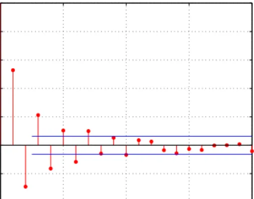
For an MA(q) process, the ACF is identically zero for lagsk greater thanq. An MA(q) process can be equally written as
θ−1(B)zt =et (3.30)
whereθ(B)is assumed to be invertible, with its inverse denoted by θ−1(q). Therefore, the PACF in an MA process has infinite components. Fig. (3.3) illustrates estimated ACF and PACF for an MA(1) process
0 5 10 15 20 −0.2 0 0.2 0.4 0.6 0.8 Lag Sample Autocorrelation
Sample Autocorrelation Function
0 5 10 15 20 −0.4 −0.2 0 0.2 0.4 0.6 0.8 1 Lag
Sample Partial Autocorrelations
Sample Partial Autocorrelation Function
Figure 3.3: ACF and PACF ofzt=et+ 0.8et−1
Clearly, AR and MA processes follow different patterns of ACF and PACF. Table 3.1 below can be used as a guide to identify AR or MA models based on the pattern of the ACF and PACF.
Table 3.1: Behaviour of Theoretical ACF and PACF for Stationary Process
Model ACF PACF
MA(q) Cuts off after lag q Exponential decay and/or damped sinusoid
AR(p) Exponential decay and/or damped sinusoid
Cuts off after lag p
ARMA(p,q) Exponential decay and/or damped sinusoid
Exponential decay and/or damped sinusoid
One major concern about the ACF and PACF approach in the case of an ARMA(p,q) process with bothp > 0andq >0is that there is uncertainty concerning model selection when examining only the ACF and PACF. Because of this, Woodward and Gray in 1981 defined the generalized partial autocorrelation (GPAC). First, letztbe a stationary process
with ACFρj, j = 0,±1,±2, . . . ,and consider the followingk×k system of equations ρj+1 =ϕ (j) k1ρj +ϕ (j) k2ρj−1+. . .+ϕ (j) k,k−1ρj−k+2+ϕ (j) kkρj−k+1 ρj+2 =ϕ (j) k1ρj+1+ϕ (j) k2ρj +. . .+ϕ (j) k,k−1ρj−k+3+ϕ (j) kkρj−k+2 .. . ρj+k =ϕ (j) k1ρj+k−1+ϕ (j) k2ρj+k−2+. . .+ϕ (j) k,k−1ρj+1+ϕ (j) kkρj (3.31)
whereϕ(j)ki denotes theith coefficient associated with thek×ksystems in whichρj+1is on
the left-hand side of the first equation. The GPAC function is defined to beϕ(j)kk. By using Cramer’s rule, it can be solved with
ϕ(j)kk = ρj . . . ρj−k+2 ρj+1 ρj+1 . . . ρj−k+3 ρj+2 .. . ρj+k−1 . . . ρj+1 ρj+k ρj . . . ρj−k+2 ρj−k+1 ρj+1 . . . ρj−k+3 ρj−k+2 .. . ρj+k−1 . . . ρj+1 ρj (3.32)
The GPAC can uniquely determine the orderspandqof an ARMA(p,q) process when the true autocorrelations are known. For an ARMA(p,q) process,ϕ(q)pp =ϕp. Also, as with
the partial autocorrelation function, it can be shown that ifk > pthenϕ(q)kk = 0. Thus, the GPAC provides identification of pand q uniquely for an ARMA(p,q) model in much the same way as the partial autocorrelation does for identification ofpfor an AR(p).
Another useful property of the GPAC is described by Woodward and Gray [41]. Letzt
be an ARMA process with autoregressive order greater than zero, then 1. ztis an ARMA(p,q) if and only ifϕ
(q) kk = 0, k > pandϕ (q) pp ̸= 0 2. ifztARMA(p,q) thenϕ (q+h) pp =ϕq, h≥0
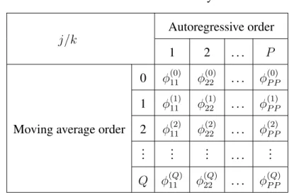
Woodward et.al [41] also recommended examining the GPAC by calculatingϕ(j)kk, k = 1,2, . . . P andj = 1,2, . . . Qfor someP andQthen placing these value in a GPAC array, as in Table 3.2.
Table 3.2: GPAC Array
j/k
Autoregressive order
1 2 . . . P
Moving average order
0 ϕ(0)11 ϕ(0)22 . . . ϕ(0)P P 1 ϕ(1)11 ϕ(1)22 . . . ϕ(1)P P 2 ϕ(2)11 ϕ(2)22 . . . ϕ(2)P P .. . ... ... . . . ... Q ϕ(Q)11 ϕ(Q)22 . . . ϕ(Q)P P
The first row of the GPAC array consists of the partial autocorrelations. We need to find a row in which zeros begin occurring beyond a certain point. This row is theqth row, and the zeros begin in the p+ 1st column. Also, values in the pth column are constant from theqth row and below. This constant isϕp ̸= 0. Given the true autocorrelation for an
ARMA(p,q) process, the patterns in the GPAC array uniquely determine the model orders if P andQare chosen sufficiently large. Table 3.3 shows the GPAC array for an ARMA(p,q) process.
Table 3.3: GPAC Array for An ARMA(p, q)Process
j/k
Autoregressive order
1 2 . . . p p+ 1 . . .
Moving average order
0 ϕ(0)11 ϕ(0)22 . . . ϕ(0)pp ϕ(0)p+1,p+1 . . . 1 ϕ(1)11 ϕ(1)22 . . . ϕ(1)pp ϕ(1)p+1,p+1 . . . .. . q−1 ϕ(q11−1) ϕ22(q−1) . . . ϕ(qpp−1) ϕ(qp+1,p+1−1) . . . q ϕ(q)11 ϕ(q)22 . . . ϕp 0 0 . . . q+ 1 ϕ(q+1)11 ϕ(q+1)22 . . . ϕp 00 00 . . . .. . ϕp 00 00 . . . 3.3.2 Parameter estimation
Once, the “order” of the model is determined, the next step is to estimate the parameters. In the ARIMA model ϕ(B)Φ(Bs)∇Ds = θ(B)Θ(Bs)et, the parameters that need to be
estimated areϕ = (ϕ1, ϕ2, . . . , ϕp)T, Φ = (Φ1,Φ2, . . . ,ΦP)T, θ = (θ1, θ2, . . . , θq)T and
Θ = (Θ1,Θ2, . . . ,ΘQ)T. The principal method for estimating the parameters is maximum
likelihood.
Let us considerN =n+dobservations assumed to be generated by an ARIMA(p, d, q). The unconditional likelihood is given by
l(ϕ, θ, σ) = f(ϕ, θ)−nlnσ− S(ϕ, θ)
2σ2 (3.33)
Here, the noise series, et, is assumed to follow a normal distribution with zero mean and
varianceσ2. f(ϕ, θ)is a function ofϕandθ. The unconditional sum of squares function is given by S(ϕ, θ) = n ∑ t=1 [et|w, ϕ, θ]2 + [e∗]′Ω−1[e∗] (3.34) Where [et|w, ϕ, θ] = E[et|w, ϕ, θ] denotes the expectation of et conditional on w, ϕ, θ.
etprocesses needed prior to timet= 1,Ωσe2 =cov(e∗)is the covariance matrix ofe∗, and [e∗] = ([w1−p], . . . ,[w0],[e1−q], . . . ,[e0])′ denotes the vector of conditional expectations (”back forecasts”) of the initial values givenw, ϕ, θ. An alternative way to represent the sum of squares is asS(ϕ, θ) = ∑nt=−∞[et]2.
Usually , f(ϕ, θ) is important only for small n. For moderate and large value of n, (3.33) is dominated by S(ϕ,θ)2σ2 . Thus, the contours of the unconditional sum of squares
function in the space of the parametersf(ϕ, θ)are very nearly contours of likelihood and of log-likelihood. In particular, the parameter estimates, obtained by minimizing the sum of squares (3.34) which we call (unconditional or exact) least squares estimates, will provide very close approximations to the maximum likelihood estimates.
S(ϕ, θ) =
n
∑
j=1
e2j (3.35)
The termf(ϕ, θ)is a function of coefficients ϕ andθ. This is small in comparison with the sum of squares functionS(ϕ, θ)when the effective number of observations,n, is large. Thus, the parameters which minimizeS(ϕ, θ)are usually used as close approximations to maximum likelihood estimates.
3.3.3 Diagnostic testing
The last step in building the ARIMA model is diagnostic testing. This step is useful to examine the adequacy of the model and to see if potential improvements are needed. Di-agnostic tests can be done through the residual analysis. The residual (one-step prediction error) for an ARMA(p,q) process can be obtained from
ˆ et =zt−( p ∑ i=1 ˆ ϕizt−i− q ∑ i=1 ˆ θeˆt−i) (3.36)
If the specified model is adequate, and the appropriate orderspandqare identified, it should transform the observations to a white noise process. Thus, the residuals should behave like white noise.
One way of checking the whiteness ofet is by checking the autocorrelation for et. If
there is only one spike at t = 0 with magnitude 1, and all the other autocorrelations are equal to zero, then et is white noise. In the other words, if the model is appropriate, the
autocorrelation should not differ significantly from zero for all lags greater than one. If the form of the model were correct and if the true parameter values are known, then the standard error of the residual autocorrelation would be n−1/2. Any residual ACF more
than two standard errors from zero would indicate that the residuals were not white, and therefore that the model orders were not accurate.
Another way to test for the whiteness of the residuals is a chi-square test of model adequacy. The test statistic is
Q=n
K
∑
k=1
re2(k) (3.37)
which is approximately chi-square distributed withK −p−q degrees of freedom if the model is appropriate. If the model is inadequate, the calculated value ofQwill be inflated. Thus, we should reject the hypothesis of model adequacy if Q exceeds an approximate small upper tail point of the chi-square distribution withK −p−qdegrees of freedom.
As explained above, these steps are iterative steps. If the fitted model is not adequate, the identification process will continue until the fitted model is adequate.
3.3.4 Forecast
If we have completed the identification process by building the ARIMA model, now we are ready to use the model to forecast future observations. If the current time is denoted byt, the forecast forzt+m is called them-step-ahead forecast and denoted byzˆt+m(t). The
standard criterion to obtain the best forecast is to minimize the mean squared error. It can be shown that the best forecast in the mean square sense is the conditional expectation of zt+m given current and previous observations:
ˆ
Let us illustrate (3.38) through this example. Consider an ARIMA (1,1,1) model (1−0.3B)(1−B)zt = (1−0.1B)et
(1−1.3B+ 0.3B2)zt = (1−0.1B)et
zt = 1.3zt−1 −0.3zt−2+et−0.1et−1
For the one step ahead forecast, replacetbyt+ 1then take the conditional expectation on both sides
zt(1) = 1.3zt−0.3zt−1+et(1)−0.1et
zt(1) = 1.3zt−0.3zt−1−0.1et
where et(1) = E[et+1|et, et−1, . . .] = E[et+1] = 0 since et is white noise. Similarly,
et(j) = 0 forj > 0. Then, for two step ahead forecasts, replacet byt+ 2 then take the
conditional expectation on both sides
zt(2) = 1.3zt(1)−0.3zt+et(2)−0.1et(1)
zt(2) = 1.3zt(1)−0.3zt
Hence, for anmstep ahead forecast, it becomes
zt(m) = 1.3zt(m−1)−0.3zt(m−2) for m >2
In general, for a given model, themstep ahead forecast can be found using the follow-ing procedures
1. expand the given model until an explicit expression forztis obtained
2. replacetbyt+mand then take the conditional expectation 3. apply the following properties to the equation obtained by step 2
![Figure 2.1: A Typical Configuration of An Electric Power System[17]](https://thumb-us.123doks.com/thumbv2/123dok_us/534573.2563055/17.892.173.748.110.770/figure-typical-configuration-electric-power.webp)
![Figure 2.2: An Input-Output Configuration of A STLF System and Its Major Uses [16]](https://thumb-us.123doks.com/thumbv2/123dok_us/534573.2563055/21.892.164.774.127.627/figure-input-output-configuration-stlf-major-uses.webp)