2018
Statistical methods for gene expression studies
using next-generation sequencing experiments
Ran Bi
Iowa State University
Follow this and additional works at:
https://lib.dr.iastate.edu/etd
Part of the
Biostatistics Commons
This Dissertation is brought to you for free and open access by the Iowa State University Capstones, Theses and Dissertations at Iowa State University Digital Repository. It has been accepted for inclusion in Graduate Theses and Dissertations by an authorized administrator of Iowa State University Digital Repository. For more information, please [email protected].
Recommended Citation
Bi, Ran, "Statistical methods for gene expression studies using next-generation sequencing experiments" (2018).Graduate Theses and Dissertations. 16790.
experiments
by
Ran Bi
A dissertation submitted to the graduate faculty in partial fulfillment of the requirements for the degree of
DOCTOR OF PHILOSOPHY
Major: Statistics
Program of Study Committee: Peng Liu, Major Professor
Daniel S. Nettleton Li Wang Zhengyuan Zhu
Chong Wang
Iowa State University Ames, Iowa
2018
DEDICATION
I would like to dedicate this thesis to my parents, Li Liu and Shoudong Bi, and to my husband Yao Chen, for their endless support and unconditional love.
TABLE OF CONTENTS
Page
LIST OF TABLES . . . vii
LIST OF FIGURES . . . ix
ACKNOWLEDGMENTS . . . xiv
ABSTRACT . . . xv
CHAPTER 1. GENERAL INTRODUCTION . . . 1
1.1 Next-generation Sequencing Technology . . . 1
1.1.1 RNA-seq . . . 1
1.1.2 Ribo-seq . . . 2
1.2 False Discovery Rate . . . 2
1.2.1 Benjamini and Hochberg Method . . . 3
1.2.2 Theq-value Procedure . . . 4
1.2.3 Bayesian FDR . . . 4
1.3 Bayesian Hierarchical Modeling . . . 5
1.4 Dissertation Organization . . . 5
Bibliography . . . 6
2. SAMPLE SIZE CALCULATION WHILE CONTROLLING FALSE DISCOVERY RATE FOR DIFFERENTIAL EXPRESSION ANALYSIS WITH RNA-SEQUENCING EXPER-IMENTS . . . 7
2.1 Introduction . . . 8
2.2 Methods . . . 12
2.2.2 The LH Method of Sample Size Calculation . . . 13
2.2.3 Proposed Method for RNA-seq Experiments with Two-sample Comparison . 15 2.3 Results and Discussion . . . 18
2.3.1 Simulation1. Same Set of Parameters . . . 18
2.3.2 Simulation 2. Gene-specific Mean and Dispersion with Fixed Fold Change . . 25
2.3.3 Simulation 3. Gene-specific Mean and Dispersion with Different Fold Change 26 2.3.4 Simulation 4. Real Data-based Simulation . . . 28
2.4 Conclusions . . . 30
2.5 Appendices . . . 33
2.5.1 Appendix A: Derivation of Equation (2.3) . . . 33
2.5.2 Appendix B: Choice of Rejection Region Γ Satisfying Formula (2.1) . . . 35
Bibliography . . . 38
3. A SEMI-PARAMETRIC BAYESIAN APPROACH, iSBA, FOR DIFFERENTIAL EX-PRESSION ANALYSIS OF RNA-SEQ DATA . . . 41
3.1 Introduction . . . 41
3.2 Bayesian Mixture Modeling . . . 44
3.2.1 A Poisson-Gamma Mixture Model . . . 44
3.2.2 Prior Specification . . . 45
3.3 Posterior Inference . . . 47
3.3.1 Markov Chain Monte Carlo Simulation . . . 47
3.3.2 Bayesian FDR Control . . . 50
3.4 Simulation . . . 51
3.4.1 Simulation A . . . 51
3.4.2 Simulation B . . . 52
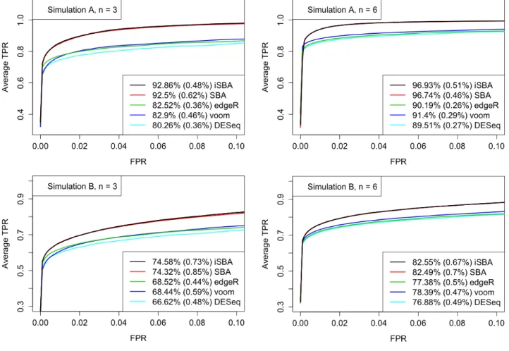
3.4.3 Simulation Results for Testing DE Genes . . . 52
3.4.4 Simulation Results for Testing: |logF C| ≤log1.5 . . . 56
3.5 Real Data Analysis . . . 58
3.6 Discussion . . . 59
3.7 Appendices . . . 61
3.7.1 Proof of Model Invariance . . . 61
3.7.2 Detailed MCMC Sampling Scheme . . . 62
Bibliography . . . 70
4. A SEMI-PARAMETRIC BAYESIAN APPROACH FOR DETECTION OF GENE EX-PRESSION HETEROSIS WITH RNA-SEQ DATA . . . 73
4.1 Introduction . . . 74
4.2 A Semi-parametric Bayesian Model . . . 76
4.2.1 A Poisson-Gamma Mixture Model . . . 77
4.2.2 Prior Specification . . . 78
4.3 Posterior Inference . . . 80
4.3.1 Markov Chain Monte Carlo Simulation . . . 80
4.3.2 Bayesian FDR for Multiple Hypothesis Testing . . . 81
4.4 Data Division . . . 82
4.5 Simulation Studies . . . 83
4.5.1 Simulation A . . . 83
4.5.2 Simulation B . . . 84
4.5.3 Simulation Results for Detecting Gene Expression Heterosis . . . 84
4.5.4 Number of Groups Divided . . . 89
4.5.5 Computational Time . . . 89
4.6 Real Data Analysis . . . 89
4.7 Discussion . . . 93
4.8 Appendices . . . 95
4.8.1 Generate Full Conditional Distributions . . . 95
Bibliography . . . 102
5. RiboZIP, A STATISTICAL METHOD FOR DETECTION OF DIFFERENTIAL TRANS-LATIONS WITH PAIRED RIBO-SEQ AND RNA-SEQ DATA . . . 106
5.1 Introduction . . . 107
5.2 Method . . . 111
5.2.1 Bayesian Modeling Pipeline . . . 111
5.2.2 Markov Chain Monte Carlo Simulation . . . 115
5.2.3 Bayesian FDR Control . . . 116 5.3 Simulation Studies . . . 117 5.3.1 Simulation A . . . 118 5.3.2 Simulation B . . . 119 5.3.3 Simulation C . . . 121 5.3.4 Simulation Results . . . 122
5.4 Real Data Analysis . . . 130
5.5 Discussion . . . 132
5.6 Appendix: Full Conditional Distributions . . . 133
LIST OF TABLES
Page
Table 1.1 Outcomes when testing mhypotheses. . . 3
Table 2.1 Outcomes when testing Ghypotheses. . . 13
Table 2.2 Sample size and anticipated average power calculated by our method and observed average power by the voom and limma pipeline while controlling FDR using q-value procedure based on parameters at differentm for three simulation settings. We also present the comparison between our method and RnaSeqSampleSize R package for simulation 2, where the right two columns are sample size and power calculated by theRnaSeqSampleSize R package. . . 21
Table 2.3 Comparison of sample size calculation methods, including the proposed method in this paper, Zhao et al. (2015)’s approach (RnaSeqSampleSize) and Wu et al. (2015)’s approach (PROPER). Results determined by our method were based on parameters estimated at m= 200. Power was eval-uated based on thevoom and limma pipeline for our method, whileedgeR
forRnaSeqSampleSize and PROPER. The computation time for each sim-ulation was calculated on a MacAir laptop with 1.3 GHz i7 CPU and 4GB RAM. . . 29
Table 3.1 Proportion of genes remaining the same declared differential expression sta-tus between two analyses that swapped the treatment and control groups for Simulations A and B, when controlling FDR at 0.05. The proportions were averaged across the 32 simulated datasets, and the percentage in each
set of parentheses is the standard deviation of the estimated proportion. . . 58
Table 4.1 Results for HPH in Simulation A. . . 88
Table 4.2 Computational time needed for each method. . . 92
Table 4.3 Number of heterosis genes detected when controlling FDR at different levels. 92 Table 4.4 Results for LPH in Simulation A. . . 99
Table 4.5 Results for HPH in Simulation B. . . 100
Table 4.6 Results for LPH in Simulation B. . . 101
LIST OF FIGURES
Page
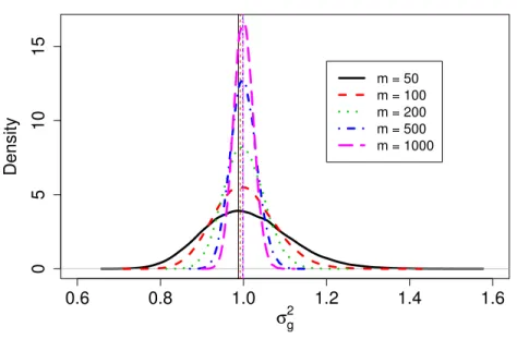
Figure 2.1 Fitted inverse gamma distributions ofσg2 for sample size m= 50, 100, 200, 500, 1000 for simulation 1. . . 20
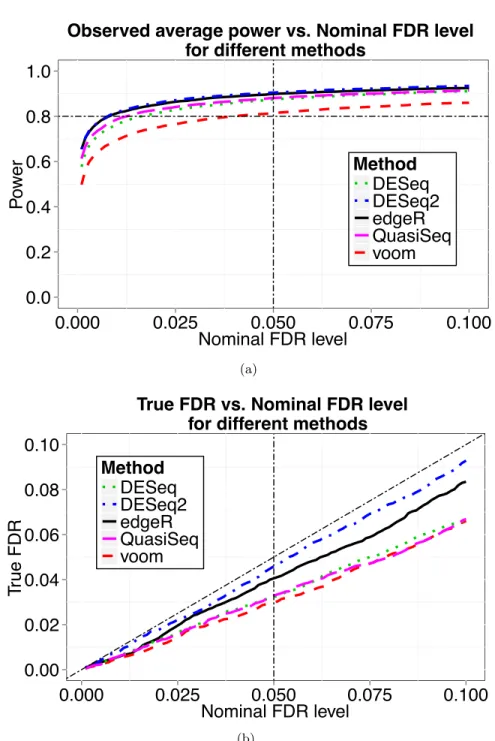
Figure 2.2 Results from simulation 1. Data were simulated with sample size n = 32. (a) Observed average power from different methods of differential expression analysis is plotted against the nominal FDR level controlled using the q-value procedure. (b) The actual FDR level versus the nominal FDR level for different methods. . . 22
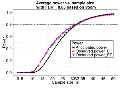
Figure 2.3 Anticipated power curve calculated byssizeRNAand observed power curves usingvoom andlimma while FDR was controlled using either the Benjamini and Hochberg method (BH) or the q-value procedure by Storey and Tibshi-rani (ST) for simulation 1. . . 23
Figure 2.4 Observed average power vs. nominal FDR for five methods at sample size
n= 20 calculated by Liet al. (2013) method for simulation 1. . . 24
Figure 2.5 Fitted inverse gamma distributions ofσ2g for sample size m = 50 and 1000 for simulation 2. . . 25
Figure 2.6 Anticipated power curve calculated byssizeRNAand observed power curves usingvoom andlimma while FDR was controlled using either the Benjamini and Hochberg method (BH) or the q-value procedure by Storey and Tibshi-rani (ST) for simulation 2 (in (a)) and 3 (in (b)). . . 27
Figure 2.7 Results from simulation 4. (a) Observed average power from different meth-ods of differential expression analysis is plotted against the nominal FDR level controlled using the q-value procedure at sample sizen= 12. (b) Antic-ipated power curve calculated byssizeRNAand observed power curves using
voom and limma while FDR was controlled using either the Benjamini and Hochberg method (BH) or the q-value procedure by Storey and Tibshirani (ST). . . 31
Figure 3.1 ROC curves resulting from Simulations A and B. For each level of FPR, the TPRs were averaged over the 32 simulated datasets. The percentage reported in the legend is the average AUC for each method, representing the percentage of 0.1, which is the total area in the range of FPR < 0.1, and the percentage in each set of parentheses is the standard deviation of the estimated AUC. . . 53
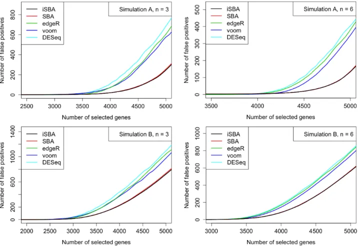
Figure 3.2 False discovery curves resulting from Simulations A and B. For each number of top ranked genes selected as DE, the number of false positives were aver-aged across the 32 simulated datasets. Genes were ranked based on either posterior probabilities orp−values. . . 54
Figure 3.3 Plots of the actual FDR versus the nominal level of FDR resulting from Simulations A and B. The dashed lines correspond to the Y = X line. A well performing method would control the FDR below or close to the dashed line. . . 55
Figure 3.4 Results for testing |logF C| ≤ log1.5 from Simulation B. The upper panel shows the ROC curves. For each level of FPR, the TPRs were averaged over the 32 simulated datasets. The percentage reported in the legend is the average AUC for each method, representing the percentage of 0.1, which is the total area in the range of FPR<0.1, and the percentage in each set of parentheses is the standard deviation of the estimated AUC. The lower panel plots the actual FDR versus the nominal level of FDR. The dashed lines correspond to the Y =X line. . . 57
Figure 3.5 The numbers of DE genes between two cell types for leaf section 4. The Venn diagram on the left shows the number of overlapping identified DE genes from our iSBA method, SBA method, and edgeR while controlling FDR at 1%; the Venn diagram on the right shows the corresponding results while controlling FDR at 5%. . . 59
Figure 4.1 ROC curves resulting from Simulations A and B. For each level of FPR, the TPRs were averaged across the 32 simulated datasets. The percentage an-notated for each method is the average AUC, represented as the percentage of the total area 0.1 in the range of FPR<0.1, and the percentage in each set of parentheses is the standard deviation of the estimated AUC. . . 86
Figure 4.2 Plots of the actual FDR versus the nominal level of FDR. When we con-trolled FDR at each nominal level, the proportion of false discoveries among the declared heterosis genes was calculated for each dataset, and the ac-tual FDR was calculated by averaging such proportions over 32 simulated datasets. The gray dash-dotted lines correspond to theY =X line. . . 87
Figure 4.3 ROC curves resulting from Simulations A and B for different data divisions. For each level of FPR, the TPRs were averaged across the 32 simulated datasets. The percentage annotated for each method is the average AUC, represented as the percentage of the total area 0.1 in the range of FPR<0.1, and the percentage in each set of parentheses is the standard deviation of the estimated AUC. . . 90
Figure 4.4 Plots of the actual FDR versus the nominal level of FDR for different data divisions. When we controlled FDR at each nominal level, the proportion of false discoveries among the declared heterosis genes was calculated for each dataset, and the actual FDR was calculated by averaging such proportions over 32 simulated datasets. The gray dash-dotted lines correspond to the
Y =X line. . . 91
Figure 4.5 Real data analysis results. The Venn diagram on the left shows the re-sults of detected HPH genes from our SBA method, eBayes laplace and
eBayes normal methods when FDR was controlled at level 0.1; the Venn diagram on the right shows the corresponding results when FDR was con-trolled at 0.05. . . 93
Figure 5.1 Histograms of pg1jk for Simulation A and B separately. . . 120
Figure 5.2 ROC curves resulting from Simulations A for different proportions of non-DTGs and various number of replicates per group. For each level of FPR, the TPRs were averaged across the 32 simulated datasets. The percentage reported in the legend is the average AUC for each method, representing the percentage of the total area 0.1 in the range of FPR<0.1, and the per-centage in each set of parentheses is the standard deviation of the estimated AUC. . . 124
Figure 5.3 ROC curves resulting from Simulations B for different proportions of non-DTGs and various number of replicates per group. For each level of FPR, the TPRs were averaged across the 32 simulated datasets. The percentage reported in the legend is the average AUC for each method, representing the percentage of the total area 0.1 in the range of FPR<0.1, and the per-centage in each set of parentheses is the standard deviation of the estimated AUC. . . 125
Figure 5.4 ROC curves resulting from Simulation C. . . 126
Figure 5.5 Plot of the actual FDR versus the nominal level of FDR for Simulation A. The proportion of false discoveries among the declared DTGs was cal-culated for each dataset when we controlled FDR at nominal levels, and the actual FDR was calculated by averaging such proportions over 32 simu-lated datasets at each nominal FDR level. The grey lines correspond to the
Y =X line. . . 127
Figure 5.6 Plot of the actual FDR versus the nominal level of FDR for Simulation B. The proportion of false discoveries among the declared DTGs was cal-culated for each dataset when we controlled FDR at nominal levels, and the actual FDR was calculated by averaging such proportions over 32 simu-lated datasets at each nominal FDR level. The grey lines correspond to the
Y =X line. . . 128
Figure 5.7 FDR plots resulting from Simulation C. . . 129
Figure 5.8 The Venn diagram for detected DTGs from our RiboZIP method (testing FC>2 or<1/2),xtail, and babel, while controlling FDR at 0.05. . . 131
Figure 5.9 The Venn diagram for detected DTGs from our RiboZIP method (testing FC>1.5 or <1/1.5), xtail, and babel, while controlling FDR at 0.05. . . 132
ACKNOWLEDGMENTS
I would like to take this opportunity to express my thanks to those who helped me with various aspects of conducting research and the writing of this thesis.
First and foremost, my sincere gratitude to my advisor, Dr. Peng Liu, who have bestowed her profound knowledge, generous support, continuous guidance, and great patience on me, during my PhD journey.
I am also very grateful to my committee members Dr. Dan Nettleton, Dr. Li Wang, Dr. Zhengyuan Zhu, Dr. Chong Wang, and Dr. Ken Koehler, for their expertise, insight and help on my dissertation research.
Thanks to Dr. Stephen Howell, Dr. Allen Miller, and Pulkit Kanodia, whom I collaborated with on my thesis projects, for their assistance and contributions.
Last but not least, I would like to thank my family and my friends for their countless love and unwavering support.
ABSTRACT
In recent years, the advancement in high-throughput next-generation sequencing technologies have revolutionized the way for genomic studies. The rapid progress of these technologies has resulted in an ever-increasing number of high-dimensional gene expression datasets available for analysis. However, due to the genetic complexity and high cost of such experiments, the number of replicates employed in an experiment is typically small. This introduces the so-called “small
n, large p” problem, where n refers to the sample size and p refers to the number of genes, in which case the power of statistical inference is limited after adjusting multiple testing errors. This dissertation presents novel statistical methods for gene expression experiments based on sequencing data, including sample size calculation and methods that allow borrow information across genes for identifying differential expressed (DE) genes, detecting gene expression heterosis, and assessing differential translation across treatments.
Chapter2proposes a one-time simulation based sample size calculation method while controlling false discovery rate (FDR) for RNA-sequencing (RNA-seq) experimental design. Our procedure is based on the weighted linear model analysis facilitated by thevoommethod, which has been shown to have competitive performance in terms of power and FDR control for RNA-seq differential expression analysis. We derive a method that approximates the average power across the DE genes, and then calculate the sample size to achieve a desired average power while controlling FDR. Simulation results demonstrate that the actual power of several popularly applied tests for differential expression is achieved and is close to the desired power for RNA-seq data with sample size calculated based on our method.
Chapter 3 develops a semi-parametric Bayesian approach for DE analysis in RNA-seq data. More specifically, we model the count data from RNA-seq experiments with a Poisson-Gamma mixture model, and propose a Bayesian mixture modeling procedure with a Dirichlet process as
the prior model for the distribution of fold changes between the two treatment means. We develop Markov chain Monte Carlo (MCMC) posterior simulation using Metropolis Hastings algorithm to generate posterior samples for differential expression analysis while controlling FDR. Simula-tion study results suggest that our proposed method outperforms other popular methods used for detecting DE genes.
In Chapter 4, we extend the idea of Chapter 3 by proposing a powerful test to detect gene expression heterosis while controlling FDR. We use the similar Poisson-Gamma mixture model for RNA-seq count data, and propose a Bayesian mixture modeling procedure with a Dirichlet process as the prior for the distribution of fold changes between each parental line versus the hybrid offspring respectively. The MCMC sampling scheme with Gibbs algorithm is utilized to provide posterior inference to detect heterosis genes while controlling false discovery rate. The effectiveness of our approach is demonstrated through simulation studies.
Chapter5addresses another gene expression analysis challenge with ribosome profiling data. It explores a new a statistical framework,RiboZIP, to identify differentially translated genes (DTGs). We model the ribosome profiling data with a zero-inflated Poisson (ZIP) model, and propose a Bayesian hierarchical modeling procedure to assess differential translation while taking the paring information between mRNA and RPFs samples into account. The MCMC sampling scheme is employed for posterior inference to detect DTGs while controlling FDR. We investigate the per-formance of our method and compare it with several existing methods used for ribosome profiling data. The analysis results show that our RiboZIP method generally provides a better ranking for genes as well as higher number of true significant results, while still adequately controlling FDR.
In summary, this dissertation raised and coped with several statistical problems under transcrip-tome data analysis. All proposed methods are evaluated through simulation studies and applied to real data analysis with fruitful results.
CHAPTER 1. GENERAL INTRODUCTION
1.1 Next-generation Sequencing Technology
Next-generation sequencing (NGS) refers to a series of sequencing technologies developed since 2005. Compared with Sanger sequencing, the first generation sequencing technologies, NGS tech-nologies simplify the library preparation, and significantly improve the sequencing throughput by utilizing massively parallel sequencing. This allows millions of fragments to be sequenced in a single run versus Sanger sequencing which only produces one forward and reverse read. During the past decade, NGS technologies have revolutionized genomic studies, and tremendous development has been made in terms of throughput, scalability, speed and sequencing cost.
1.1.1 RNA-seq
Many applications arise based on NGS technologies. RNA-Sequencing (RNA-seq), also called Whole Transcriptome Shotgun Sequencing (WTSS), is a technology that uses the capabilities of NGS to study the entire transcriptome through the sequencing of RNA molecules. In a typical RNA-seq experiment, messenger RNA (mRNA) molecules are extracted from samples, fragmented, and reverse transcribed to double-stranded complementary DNA (cDNA). The cDNA fragments are then sequenced on a high-throughput platform, such as HiSeq by Illumina or SOLiD by Applied Biosystems. After sequencing, millions of DNA fragment sequences, called reads, are recorded and aligned to a reference genome. The number of reads mapped to each gene measures the expression level for that gene.
Compared with microarray technologies that used to be the major tool for transcriptome studies, RNA-seq technologies have several advantages including a larger dynamic range of expression levels, less noise, higher throughput, and more power to detect gene fusions, single nucleotide variants and
novel transcripts. Hence, RNA-seq technologies have been popularly applied in transcriptomic studies.
1.1.2 Ribo-seq
Ribosome profiling (Ribo-seq), also named Ribosome footprinting, is a method based on NGS technologies that uses deep sequencing of ribosome-protected mRNA fragments (RPFs) to deter-mine what proteins are being actively translated in a cell.
It is a modification of RNA-seq that allows one to essentially detect the position and amount of every translating (80S) ribosome on every mRNA in the sample. Briefly, a translation-arrested cell lysate is digested with RNase to degrade all mRNA that is not protected by a translating ribosome. The resulting RPFs, along with randomly fragmented total RNA from the same initial lysate to be used for normalization, are sequenced by Illumina sequencing, then mapped to the reference genome or transcriptome. RPFs represent the mRNA region occupied by the translating ribosome (Ingoliaet al., 2009). The positions and numbers of RPFs on each mRNA indicate the abundance of ribosomes at each position in each mRNA. Highly translated mRNAs and ribosome pause sites generate more RPFs. Therefore, the number of RPFs mapped on the coding region of an mRNA species has been frequently used as a measurement of the level of translation.
1.2 False Discovery Rate
Both RNA-seq and Ribo-seq technologies measure tens of thousands of genes. A major goal in the analysis of gene expression is to identify genes that are of interest, such as genes whose expression levels change across conditions, or whose translational efficiency changes across conditions. Thus multiple testing procedures that control the number of false significant results while simultaneously testing a large number of hypotheses is essential. Assume there arem genes in total and each gene is tested of a hypothesis. Among themtests, supposem0 of the null hypotheses are true andm1 of
represent the p-values correspond to the m tests. Also, we denote p(1), . . . , p(m) as the ordered
p-values from smallest to largest.
We rejectH0i ifpi ≤cand fail to reject H0i ifpi> c, where the cutoff valuecis chosen in order
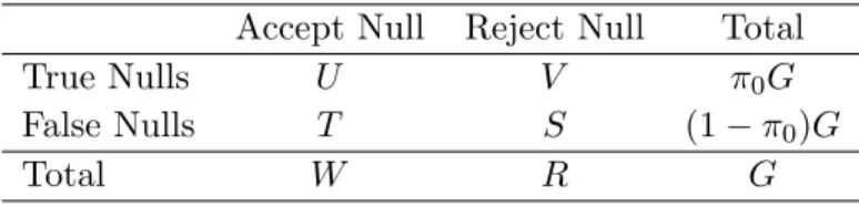
to control some type of error rate. Table 1.1 summarizes the various outcomes that occur when testing m hypotheses, whereV is the number of false positives, R is the number of rejections.
Table 1.1 Outcomes when testingm hypotheses.
Accept Null Reject Null Total
True Nulls U V m0
False Nulls T S m1
Total W R m
False discovery rate (FDR), defined by Benjamini and Hochberg (1995), is the expected pro-portion of false positives among the rejected hypothesis,
F DR=E V R R >0 P r(R >0),
has been the choice of error criterion in genomic studies. There are several well known and com-monly used methods for controlling FDR (choosing c).
1.2.1 Benjamini and Hochberg Method
Benjamini and Hochberg (1995) proposed a method for controlling FDR at level α by finding the largest integerk such that
p(k) ≤ kα
m, (1.1)
and setting c =p(k). If no such k exists, then set c = 0 and no hypotheses testings are rejected. Notice that the Benjamini and Hochberg (1995) method controls FDR at level α(m0/m) rather
1.2.2 The q-value Procedure
An improved method for controlling FDR at level α would be to replace the quantity m with
m0 in1.1, butm0 needs to be estimated since it is unknown. Storey (2002) proposed a method to
estimate quantitym0 with ˆm0, and defined theq-value as q(j)=min p (r)mˆ0 r :r=j, . . . , m ,
whereq(j)is theq-value corresponds to the gene with thejthsmallestp-value, andqj corresponds to
theq-value ofjth hypothesis testing. Theq-value converts thep-value from a significance measure of the Type I error rate of a single hypothesis test to a significance measure of the FDR for a family of mhypothesis tests.
1.2.3 Bayesian FDR
The Bayesian version of FDR is an alternative way to estimate the FDR within the Bayesian framework. It has been proposed and discussed by several authors including Genovese and Wasser-man (2003) and Newton et al. (2004). The Bayesian FDR can be obtained by using posterior probabilities of the null hypotheses. More specifically, for each hypothesis i, i= 1, . . . , m, we de-note the posterior probability that ith null hypothesis is true by vi. vi can be estimated by the
proportion of the posterior samples for some parameters or some function of parameters that falls into the null set ∆0. We rejectH0i if the estimated posterior probability ˆvi is smaller than a critical
value c∗. The critical value c∗ is chosen based on controlling the FDR below a target levelα, for example, 0.05, i.e., c∗ =sup{c:F DR\(c)< α}, where \ F DR(c) = Pm i=1ˆviI(ˆvi< c) Pm i=1I(ˆvi < c) .
So the Bayesian FDR controlled at levelα can be calculated by
\ BF DR(α) = Pm i=1ˆviI(ˆvi < c∗) Pm i=1I(ˆvi< c∗) .
1.3 Bayesian Hierarchical Modeling
For genomic studies, tens of thousands of genes are simultaneously measured for their expression levels. However, due to the genetic complexity and high-dimensionality of the resulting datasets, in addition to the cost of experimental materials and sequencing, many experiments only employ a small number of replicates. This introduces the “small n, large p” problem, where nrefers to the sample size andprefers to the number of variables, in which cases the power of statistical inference is limited after adjusting multiple testing errors. Therefore, in order to mitigate the effects of small sample sizes during estimation, Bayesian hierarchical modeling approach has been proposed in terms of borrowing information across genes, and is becoming increasingly popular in statistical genomics (Do et al., 2005; Hardcastle and Kelly, 2010; Wuet al., 2012).
1.4 Dissertation Organization
In the rest of this dissertation, each chapter addresses one challenge related to RNA-seq or Ribo-seq analysis. In Chapter 2, we propose a procedure for sample size calculation while controlling FDR for RNA-seq experimental design. Chapter3 extends Liu et al.(2015) idea, and develops a semi-parametric Bayesian approach for differential expression analysis of RNA-seq data. Chapter
4 uses the method introduced in Liuet al.(2015) and Chapter 3, and proposes a semi-parametric Bayesian approach for detection of gene expression heterosis while controlling FDR. In Chapter5, we utilize a zero-inflated Poisson (ZIP) model and adopt a Bayesian hierarchical modeling pipeline to assess differential translations with ribosome profiling data.
Bibliography
Benjamini, Y., Hochberg, Y.(1995). Controlling the false discovery rate: a practical and powerful approach to multiple testing. J. R. Stat. Soc. B,57, 289–300.
Do, K. A. , Muller, P., Tang, F. (2005). A Bayesian Mixture Model For Differential Gene. Journal of the Royal Statistical Society, Series C (Applied Statistics),54, 627–644.
Genovese, C., Wasserman, L. (2003). Bayesian and Frequentist Multiple Testing.Bayesian Statis-tics,7, 145–161.
Hardcastle, T. J., Kelly, K. A. (2010). baySeq: Empirical Bayesian Methods for Identifying Differ-ential Expression in Sequence Count Data.BMC Bioinformatics,11, 422.
Ingolia, N. T., Ghaemmaghami, S., Newman, J. R. S., Weissman, J. S.(2009). Genome-wide analysis in vivo of translation with nucleotide resolution using ribosome profiling. Science,324, 218–23. Liu, F., Wang, C., Liu, P. (2015). A Semi-parametric Bayesian Approach for Differential Expression
Analysis of RNA-seq Data. J Agric Biol Environ Stat,20(4), 555–576.
Newton, M. A., Noueiry, A., Sarkar, D., Ahlquist, P. (2004). Detecting Differential Gene Expression with a Semiparametric Hierarchical Mixture Method. Biostatistics,5, 155–176.
Storey, J. D. (2002). A Direct Approach to False Discovery Rates. Journal of the Royal Statistical Society, Series B,64, 479–498.
Wu, H., Wang, C., Wu, Z. (2012). A new shrinkage estimator for dispersion improves differential expression detection in RNA-seq data. Biostatistics,1(1), 1–24.
CHAPTER 2. SAMPLE SIZE CALCULATION WHILE CONTROLLING FALSE DISCOVERY RATE FOR DIFFERENTIAL EXPRESSION
ANALYSIS WITH RNA-SEQUENCING EXPERIMENTS
Published in BMC Bioinformatics 2016, 17:146
Ran Bi, Peng Liu
Abstract
Background: RNA-Sequencing (RNA-seq) experiments have been popularly applied to transcrip-tome studies in recent years. Such experiments are still relatively costly. As a result, RNA-seq experiments often employ a small number of replicates. Power analysis and sample size calculation are challenging in the context of differential expression analysis with RNA-seq data. One challenge is that there are no closed-form formulae to calculate power for the popularly applied tests for differential expression analysis. In addition, false discovery rate (FDR), instead of family-wise type I error rate, is controlled for the multiple testing error in RNA-seq data analysis. So far, there are very few proposals on sample size calculation for RNA-seq experiments.
Results: In this paper, we propose a procedure for sample size calculation while controlling FDR for RNA-seq experimental design. Our procedure is based on the weighted linear model analysis facilitated by the voom method which has been shown to have competitive performance in terms of power and FDR control for RNA-seq differential expression analysis. We derive a method that approximates the average power across the differentially expressed genes, and then calculate the sample size to achieve a desired average power while controlling FDR. Simulation results demon-strate that the actual power of several popularly applied tests for differential expression is achieved and is close to the desired power for RNA-seq data with sample size calculated based on our method.
Conclusions: Our proposed method provides an efficient algorithm to calculate sample size while controlling FDR for RNA-seq experimental design. We also provide an R package ssizeRNA that implements our proposed method and can be downloaded from the Comprehensive R Archive Network (http://cran.r-project.org).
Keywords: RNA-seq; FDR; Experimental design; Sample size calculation; Power analysis.
2.1 Introduction
During the past decade, next generation sequencing (NGS) technology has revolutionized ge-nomic studies, and tremendous development has been made in terms of throughput, scalability, speed and sequencing cost. RNA-Sequencing (RNA-seq), also called Whole Transcriptome Shot-gun Sequencing (WTSS), is a technology that uses the capabilities of NGS to study the entire transcriptome. Compared with microarray technologies that used to be the major tool for tran-scriptome studies, RNA-seq technologies have several advantages including a larger dynamic range of expression levels, less noise, higher throughput, and more power to detect gene fusions, single nu-cleotide variants and novel transcripts. Hence, RNA-seq technologies have been popularly applied in transcriptomic studies.
In a typical RNA-seq experiment, messenger RNA (mRNA) molecules are extracted from sam-ples, fragmented, and reverse transcribed to double-stranded complementary DNA (cDNA). The cDNA fragments are then sequenced on a high-throughput platform, such as HiSeq by Illumina or SOLiD by Applied Biosystems. After sequencing, millions of DNA fragment sequences, called reads, are recorded and aligned to a reference genome. The number of reads mapped to each gene measures the expression level for that gene. Thus, RNA-seq provides discrete count data serving as measurements of mRNA expression levels, which is different from the fluorescence intensity mea-surements from microarray technologies that have been considered as continuous variables after transformation. As a result of high frequency of low integers, the statistical methods developed for analyzing microarray data are not directly applicable for RNA-seq data.
In the statistical analysis of RNA-seq data, identifying differentially expressed (DE) genes across treatments or conditions is a major step or main focus. A gene is considered to be DE across treatments or conditions if the mean read counts differ across treatment groups. Otherwise, we say the gene is equivalently expressed (EE). Many statistical methods have been proposed for the detection of DE genes with RNA-seq data. Some popular methods, includingedgeR(Robinson and Smyth, 2007, 2008; Robinsonet al., 2010; McCarthyet al., 2012),DESeq(Anders and Huber, 2010) and DESeq2 (Love et al., 2014), are based on the negative binomial (NB) distribution. QuasiSeq
(Lundet al., 2012) presented quasi-likelihood methods with shrunken dispersion estimates. A more recently proposed method by the Smyth group (Lawet al., 2014) works with log-transformed count data and captures the mean-variance relationship of the log-count data through a precision weight for each observation (using a function calledvoom in their R package) and then applies the limma
method (Smyth, 2004) for differential expression analysis.
Due to the genetic complexity and high-dimensionality of the resulting datasets, RNA-seq periments require complicated bioinformatic and statistical analysis in addition to the cost of ex-perimental materials and sequencing. Many experiments only employ a small number of replicates, in which cases the power of statistical inference is limited. However, if the sample size is too large (which is rare), it is also a waste of experimental materials and manpower. For these reasons, one of the principal questions in designing an RNA-seq experiment is: how many biological replicates should be used to achieve a desired power? In other words, how large of the sample size do we need?
To answer this question, we need to determine a sample size that is required to achieve a desired power while controlling an appropriate error rate. When calculating sample size for a single test, type I error rate is commonly used. Fang and Cui (2011) discussed a sample size formula for a single gene based on likelihood ratio test or Wald test. Hartet al.(2013) and their associated R package
RNASeqPower (Therneau et al., 2015) proposed a sample size calculation method for any single gene based on score test while controlling type I error rate. However, for RNA-seq data analysis, tens of thousands of genes are simultaneously tested for differential expression, which requires the
correction of multiple testing error, and false discovery rate (FDR) (Benjamini and Hochberg, 1995) has been the choice of error criterion in RNA-seq data analysis.
Several sample size calculation methods while controlling FDR have been proposed in microarray experiments. For example, Liu and Hwang (2007) developed a method to calculate sample size given a desired power and a controlled level of FDR by finding the rejection region for the test procedure and hence power for each sample size. Hereafter, we call this sample size calculation method the LH method. Orr and Liu (2009) assembled thessize.fdr R package which implements the LH method. However, sample size calculation for RNA-seq data analysis while controlling FDR is underde-veloped. Some earlier studies performed sample size and power estimation for RNA-seq experiments under Poisson distribution (Chen et al., 2011; Busby et al., 2013; Li et al., 2013), but the addi-tional biological variation across RNA-seq samples yields overdispersion, which means the equal mean-variance relationship for the Poisson distribution does not adapt to the variability present in RNA-seq data. To account for overdispersion, the negative binomial distribution is more flexible to use. Liet al.(2013) proposed a sample size determination method while controlling FDR based on the exact test implemented in edgeR that tests for genes differentially expressed between two treatments or conditions. This method calculates a sample size based on the minimum fold change of DE genes, the minimum average read counts of DE genes in the control group, and the maximum dispersion of DE genes under negative binomial models. As expected, such a method would be very conservative and not practically informative. TheRnaSeqSampleSize R package (Zhaoet al., 2015) provides an estimation of sample size based on single read count and dispersion which implements Li et al. (2013) method. Also, instead of using the minimum average read counts and the maxi-mum dispersion,RnaSeqSampleSizegives an estimation of sample size based on the read count and dispersion distributions estimated from real data, together with the minimum fold change, which is much better than Li et al. (2013) method, but would still be conservative due to the usage of the minimum fold change. The LH method is applicable as long as we can compute the power and type I error rate given a rejection region. However, there are no closed-form formulae for power for the popularly applied NB based methods. Then we have to rely on a lot of simulation to figure
out quantities such as power and type I error rate for each sample size and each simulation setting (Fang and Cui, 2011). Chinget al.(2014) provided a power analysis tool that calculates the power for a given budget constraint for each size of samples, and then determined the sample size for a desired power. Wu et al. (2015) introduced the concepts of stratified targeted power and false discovery cost, and estimated sample size by the evaluation of statistical power over a range of sample sizes based on simulation studies. Both Chinget al. (2014) and Wuet al.(2015) methods are simulation-based, thus we need to do a lot of simulations for power assessment for each sample size, which is time-consuming.
In this paper, we propose a much less computationally intensive method, which only demands one-time simulation, for sample size calculation in designing RNA-seq experiments. First, we use the voom method to model the mean-variance relationship of the log-count data of RNA-seq and produce a precision weight for each observation. Second, based on the normalized log-counts and associated precision weights, we estimate the distribution of weighted residual standard deviation of expression levels. Then for two-sample experiments, we derive a formula of the t test statistic in the weighted least squares setting and estimate the distribution of effect size for differential expression. Next, we apply the LH method to calculate the required sample size for a given desired power and a controlled FDR level. Our simulation demonstrates that the desired power is reached for data with the sample size calculated from our method for several popular tests for differential expression.
The article is organized as follows. The Methods section (Section 2.2) describes our proposed method illustrated with the two-samplet-test. In the Results and Discussion section (Section2.3), we present four simulation studies based on either negative binomial distributions or real RNA-seq dataset, and our method provide reliable sample sizes for all simulation studies. The Conclustions section (Section2.4) discusses our results and some future work.
2.2 Methods
In this section, we first review thevoom method (Lawet al., 2014) and the LH method of sample size calculation. Then, we introduce our approach for calculating sample size while controlling FDR in designing RNA-seq experiments.
2.2.1 The voom Method
Suppose that an RNA-seq experiment includes a total of N samples. Each sample has been sequenced, and the resulting reads are aligned with a reference genome. The number of reads mapped to each reference gene is recorded. The RNA-seq data then consist of a matrix of read counts rgij, where g = 1,2, . . . , G denotes gene g, i = 1,2 denotes group where i = 1 is for the
control group and i= 2 is for the treatment group, and j = 1,2, . . . , ni denotes replicates in each
group with N = n1 +n2. The idea of the voom method proposed by Law et al. (2014) is to use
precision weights to account for the mean-variance relationship and apply weighted least square analysis to RNA-seq data.
The method of voom starts from transforming the RNA-seq count data to the log-counts per million (log-cpm) value calculated by
ygij =log2 rgij+ 0.5 Rij + 1 ×10⁶ ,
whereRij =PGg=1rgij is the library size for theith treatment andjth replicate. As has been done
in Smyth (2004), Law et al. (2014) then fit a linear model to the transformed data according to the experimental design. For each gene g, the following linear model
yg =Xβg+εg
is fitted to yg = (yg11, . . . , yg1n1, yg21, . . . , yg2n2)0, the vector of log-cpm values, where X is the
design matrix with rows xTij, βg is a vector of parameters that may be parameterized to include log2-fold changes between experimental conditions, and εg is the error term withE(εg) =0.
Assuming that E(ygij) =µgij =xTijβg, then by ordinary least squares, the above linear model
is fitted for each geneg, which yields regression coefficient estimates βˆg, fitted values ˆµgij=xTijβˆg,
residual standard deviationsηg and fittedlog2-read counts
ˆ
lgij = ˆµgij+log2(Rij+ 1)−log2(106).
To obtain a smooth mean-variance trend, Law et al. (2014) fit a LOWESS curve to the square root of residual standard deviations η1/2g as a function of average log-counts ˜rg, where ˜rg = ¯yg+ log2( ˜R+ 1)−log2(106) with ¯yg being the average log-cpm value for each gene g and ˜R being the
geometric mean of library sizes. Then for each observation ygij, the predicted square root residual
standard deviation ˆη1/2gij is obtained to be the LOWESS fitted value corresponding to ˆlgij.
Finally, the voom precision weights are defined as the inverse variances wgij = ηˆ21
gij
. Lawet al.
(2014) recommended analyzing the log-cpm data with weighted least squares, and the weights (wgij) are used to account for the mean-variance relationship in the log-cpm values. Assuming
normal distribution for residual errors (εg), methods such ast-tests or moderatedt-tests can then
be applied for differential expression analysis.
2.2.2 The LH Method of Sample Size Calculation
In genomic studies, we simultaneously test a large number of hypotheses, each relating to a gene. Hence, multiple testing is commonly used in the analysis. Assume there areGgenes in total and each gene is tested for the significance of differential expression. Table 2.1 summarizes the various outcomes that occur when testingGhypotheses, where V is the number of false positives,
R is the number of rejections among the G tests, and π0 is the proportion of non-differentially
expressed genes.
Table 2.1 Outcomes when testing G hypotheses.
Accept Null Reject Null Total
True Nulls U V π0G
False Nulls T S (1−π0)G
False discovery rate (FDR), defined by Benjamini and Hochberg (1995), is the expected pro-portion of false positives among the rejected hypothesis:
F DR=E V R R >0 P r(R >0),
while positive FDR (pFDR), proposed by Storey Storey (2002), is defined to be
pF DR=E V R R >0 .
Both FDR and pFDR are widely used error rates to control in multiple testing encounted in genomic studies. In RNA-seq experiments, most often we end up detecting DE genes, i.e. R >0. Hence, in this paper, we do not differentiate between FDR and pFDR.
Liu and Hwang (2007) proposed a method for a quick sample size calculation for microarray experiments while controlling FDR. LetH = 0 represent no differential expression (null hypothesis is true) andH= 1 represent differential expression (null hypothesis is false). Based on the definition of pFDR and assumptions in Storey (2002) (all tests are identical, independent and Bernoulli distributed withP r(H = 0) =π0, whereπ0 is the proportion of EE genes), they derived that
α 1−α 1−π0 π0 ≥ P r(T ∈Γ|H = 0) P r(T ∈Γ|H = 1), (2.1)
whereαis the controlled level of FDR,T denotes the test statistic and Γ denotes the rejection region of the test. Then for each comparison, the LH method calculates the sample size as follows. First, for a fixed proportion of non-differentially expressed genes, π0, and the level of FDR to control,α,
they find a rejection region Γ that satisfy (2.1) for each sample size. Then for the selected rejection region Γ for each sample size, the power is calculated by P r(T ∈ Γ|H = 1). According to the desired power, a sample size is determined.
The rejection region depends on the test applied for differential expression, and the method based on (2.1) can be applied to any multiple testing procedure where the same rejection region is used. This LH method can be implemented using an R package,ssize.fdr, developed by Orr and Liu (2009), and applied for designing one-sample, two-sample, or multi-sample microarray experiments. The method would be applicable to RNA-seq experiments if we can calculate power and type I error rate given a rejection region.
2.2.3 Proposed Method for RNA-seq Experiments with Two-sample Comparison
For the popularly applied tests in RNA-seq differential expression analysis such as edgeR and
DESeq, there are no closed-form expressions to calculate the two quantities P r(T ∈ Γ|H = 0) and P r(T ∈ Γ|H = 1). Hence, the LH method cannot be directly applicable to these methods. However, the recently proposed voom and limma analysis for RNA-seq data (Law et al., 2014; Ritchie et al., 2015) is based on weighted linear models and we can obtain tractable formulae for power and type I error rate. In this paper, our idea is to derive formulae to calculate power and type I error rate based onvoom and weighted linear model analysis, and then apply the LH method for sample size calculation. We will use two-sample t-tests to illustrate our idea. Similar methods can be derived for other designs such as paired-sample or multiple treatments comparison.
Suppose our interest is to identify the differentially expressed (DE) genes between a treatment and a control group. Assuming that for gene g, group iand replicates j, we observe the RNA-seq data read counts rgij, where the mean for gene g in groupi is λgij =dijγgi. Here, dij stands for
a normalization factor or effective library size that adjusts the sequencing depth for sample j in group i, γgi stands for the normalized mean expression level of gene g in group i. Then for each
geneg, to test for differential expression means to test the hypothesis:
H0g :γg1=γg2 vs. H1g :γg16=γg2.
As reviewed in the first part of the Methods section, when applying the voom method, the RNA-seq read counts rgij are transformed to log-cpm valuesygij with associated weightswgij and
mean µgi for each sample j in group i. With this parameterization, testing for DE means testing
H0g :µg1 =µg2 vs. H1g :µg1 6=µg2,
where µg1 and µg2 are the expectation of log-cpm values of gth gene for control and treatment
group, respectively.
For each individual gene g, the weighted linear model
yg =Xβg+σgW −1
2
can be fitted to log-cpm values
yg = (yg11, . . . , yg1n1, yg21, . . . , yg2n2)
with design matrix
X= 1 0 .. . ... 1 0 1 1 .. . ... 1 1 , coefficients vector βg = βg1 βg2 ,
unknown gene-specific standard deviation σg, and associated voom precision weights
Wg =diag(wg11,· · ·, wg1n1, wg21,· · · , wg2n2).
Assuming∼M V N(0, In1+n2), where MVN stands for multivariate normal distribution, thet-test
statistic for geneg is
Tg =
ˆ
βg2 S.E.( ˆβg2)
, (2.2)
where the estimated log2-fold change between treatment and control group ˆβg2 and its standard
errorS.E.( ˆβg2) could be obtained through weighted least squares estimation.
To make thet-test based method more straightforward to apply, we reparameterize the formula (2.2) to Tg = ∆g sg q 1 n1 + 1 n2 , (2.3) where sg = s (yg−Xβg)0Wg(yg−Xβg) n1+n2−2
can be viewed as the pooled sample standard deviation, which is an estimator ofσg, and ∆g ≡βˆg2 s ¯ wg1·w¯g2· ¯ wg·· (2.4) can be viewed as the scaled effect size which is defined by weighted mean difference of log-cpm values. Here, ¯wg1·= n11 Pn1j=1wg1j, ¯wg2·= n21 Pj=1n2 wg2j and ¯wg·· = n1+n21 P2i=1Pnj=1i wgij. Details
of the derivation for (2.3) is provided in the Appendix A (2.5.1).
After generating the effect size ∆g, and the standard deviation σg for each gene g, we could
assume, as in Liu and Hwang (2007), that the effect size follows a normal distribution ∆g∼N(µ∆, σ2∆),
and the variance of log-cpm values for each gene follows an inverse gamma distribution
σg2∼Inv−Gamma(a, b)
with mean a−1b . Then we apply the LH method to calculate the optimal sample size given desired power and controlled FDR level. See Appendix B for a brief review of the calculations in the LH method involving in choosing the rejection region Γ safisfying formula (2.1).
Our proposed method requires the estimation of hyperparameters µ∆, σ∆, a, and b. If a
relatively large pilot dataset is available, these parameters can be estimated based on the pilot data. Otherwise, we can simulate data to obtain the values for these hyperparameters. It has been shown that the NB model fits real RNA-seq data well (Anders and Huber, 2010). In addition, many popularly applied tests for differential expression analysis of RNA-seq data are based on NB models. Hence, we suggest to simulate data according to NB models, and then use such simulated data to obtain the estimates ofµ∆,σ∆,a, andb, which are then used to calculate sample size. We
outline our proposed procedure for sample size calculation as follows: 1. For a given RNA-seq experiment, specify the following parameters:
G: total number of genes for testing;
π0: proportion of non-DE genes; α: FDR level to control;
pow: desired average power to achieve;
λg: average read count for gene g= 1, . . . , G in control group (without loss of generality, we
assume that the normalization factorsdij are equal to 1 for all samples); φg: dispersion parameter for geneg;
δg: fold change for gene g.
Note thatλg and φg could be estimated from real data using methods such as edgeR.
2. Simulate RNA-seq read count data from a NB distribution with given parameters in step 1. 3. Use the voom and limma method to obtain the log-cpm value and the associated precision
weight for each count, and then estimate effect size ∆g according to (2.4) for each geneg and
parameters a,b for the prior ofσg.
4. Estimateµ∆ and σ∆ by fitting
∆g ∼N(µ∆, σ∆2).
5. Use the LH method to determine the sample size n to achieve desired power and controlled FDR level.
2.3 Results and Discussion
In this section, we present four simulation studies to evaluate our proposed method for sample size calculation for RNA-seq experiments. In the first three simulation studies, we set the total number of genes to beG= 10,000 and the desired average power to be 80%. The last simulation is real data-based.
2.3.1 Simulation1. Same Set of Parameters
We start from the simplest simulation setting where all genes share the same set of parameters for the NB distribution. Although such cases are unrealistic, they allow the method of Li et al.
(2013) to perform best because this method uses a single set of NB parameters (mean, dispersion, fold change) when calculating sample size. Hence, we use this simulation setting to study the
performance of our method and compare it to the method of Li et al. (2013). We refer to the parameter settings from Table 1 in Li et al. (2013), and compare the resulting sample size and power calculated by both Li et al.(2013) method and our proposed method.
In the main manuscript, we present results for one of those parameter settings as an example: the proportion of non-DE genes π0 = 0.99, the mean read counts for control group λ = 5 with
normalization factors dij = 1, dispersion parameter φ = 0.1, FDR controlling at level 0.05, and
fold change δ = 2 for differentially expressed genes. Suppose rgij denotes the read count for gene g, group iand replicatej = 1,2, . . . , ni in each group withn1=n2=n. Then, for EE genes, both rg1j andrg2j were drawn from N B(5,0.1); for DE genes,rg1j were drawn fromN B(5,0.1) andrg2j
were drawn fromN B(10,0.1) orN B(2.5,0.1).
After setting these simulation parameters in step 1, we follow steps 2-4 to simulate data and obtain the values of hyperparameters. To investigate the effect of this simulation step, we tried different sizes of simulated data, m = 50,100,200,500,1000, where m is the sample size for each group in step 2 of our procedure. For eachm, we generated read countsrg1j(control group) andrg2j
(treatment group) from independent NB distributions for every geneg and samplej,g= 1, . . . , G,
j = 1, . . . , m. After using voom and lmFit in the R package limma (Smyth, 2004) to produce weights wgij for each observation, we then obtained effect size ∆g for each gene and parameters a,b for the prior distribution of σ2g. The fitted inverse gamma distributions of σg2 for each m are shown as in Figure 2.1, with vertical lines indicating the modes. It seems that the mode doesn’t change much, and the distribution ofσ2
g shrinks towards the center as sample size gets larger.
After obtaining the fitted parameters, we calculated sample size according to our proposed method described in the third part of the Methods section to achieve a desired power of 80%. We then simulated data according to each calculated sample size and checked whether the desired power was achieved. In Table 2.2, the first three columns listed our simulation results corresponding to this simulation setting. Asmincreased from 50 to 100 to 1000, the calculated sample size dropped from 35 to 34 and 32, respectively. This decrease is expected because the parameters were estimated more precisely with largerm. For example, the distribution ofσ2g shrank asm increased as shown
0.6 0.8 1.0 1.2 1.4 1.6 0 5 10 15 σ g 2 Density m = 50 m = 100 m = 200 m = 500 m = 1000
Figure 2.1 Fitted inverse gamma distributions ofσg2 for sample sizem= 50, 100, 200, 500, 1000 for simulation 1.
in Figure 2.1. The effect on the resulting sample size is not big, at most with a difference of 3 (35 vs. 32).
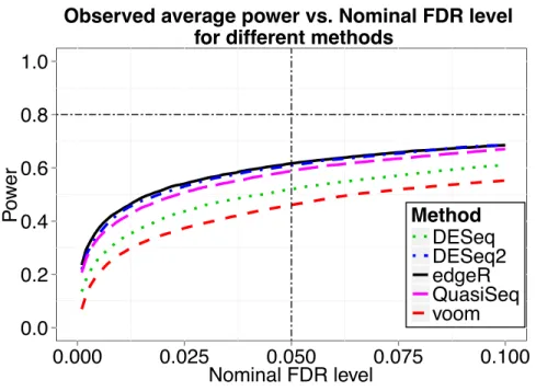
We now choose a sample size n = 32 and demonstrate this sample size indeed reaches the desired power 0.8. At n= 32, we simulated 100 datasets and performed several popularly applied tests such as the edgeR exact test, the voom and limma method, DESeq, DESeq2 and QuasiSeq
using the corresponding R packages. Desired power (0.8) was achieved for all testing methods when controlling FDR at 0.05 using q-value procedure Storey et al. (2004), and the observed FDR was controlled successfully under all the five methods. The results are shown in Figure 2.2. For the
voom andlimma pipeline method, the observed power curves while FDR was controlled using the Benjamini and Hochberg (1995) method and the q-value procedure (Storey et al., 2004) and the power curve based on our calculation are shown in Figure 2.3. The observed power was obtained by averaging actual power over 100 simulated datasets for each sample size. The observed power and the power calculated by our method are close with our calculation being a little conservative.
T able 2.2 Sample size and an ticipated a v erage p o w er calculated b y our metho d an d ob-serv ed a v erage p o w er b y the vo om and limma pip eline while con trolling FDR using q-v alue pr o cedure based on par am eters at differen t m for three sim ulation settings. W e also prese n t the comparison b et w e en our metho d and R n aSe qSam-pleSize R pac k age for sim ulation 2, where the righ t tw o columns are sample size and p o w er calculated b y the R naS eqSampleSize R pac k age. Sim ulation 1 Sim ulation 2 Sim ulation 3 Our Metho d Our Metho d R naSe qSampleSize Our Metho d m Sample An ticipated Observ ed Sample An ticipated Observ ed Sample Estimated Sample An ticipated Observ size p o w er p o w er size p o w er p o w er size p o w er size p o w er p 50 35 0.802 0.858 13 0.810 0.876 9 0.780 22 0.800 0.801 100 34 0.814 0.846 13 0.814 0.876 9 0.724 22 0.803 0.801 200 34 0.815 0.846 13 0.823 0.876 9 0.765 22 0.804 0.801 500 33 0.817 0.833 13 0.827 0.876 9 0.769 22 0.805 0.801 1000 32 0.800 0.804 13 0.826 0.876 9 0.764 22 0.805 0.801
0.0
0.2
0.4
0.6
0.8
1.0
0.000
0.025
0.050
0.075
0.100
Nominal FDR level
P
o
w
er
Method
DESeq
DESeq2
edgeR
QuasiSeq
voom
Observed average power vs. Nominal FDR level
for different methods
(a) 0.00 0.02 0.04 0.06 0.08 0.10 0.000 0.025 0.050 0.075 0.100 Nominal FDR level Tr ue FDR Method DESeq DESeq2 edgeR QuasiSeq voom
True FDR vs. Nominal FDR level for different methods
(b)
Figure 2.2 Results from simulation 1. Data were simulated with sample size n = 32. (a) Observed average power from different methods of differential expression analysis is plotted against the nominal FDR level controlled using the q-value procedure. (b) The actual FDR level versus the nominal FDR level for different methods.
Hence, our proposed method provides an accurate estimate of power, and the sample size calculated by our method is reliable.
0.0 0.2 0.4 0.6 0.8 1.0 3 5 10 15 20 25 3032 35 40 45 50 Sample size (n) P o w er Power Anticipated.power Observed.power_BH Observed.power_ST
Average power vs. sample size with FDR = 0.05 based on Voom
Figure 2.3 Anticipated power curve calculated by ssizeRNA and observed power curves using voom and limma while FDR was controlled using either the Benjamini and Hochberg method (BH) or the q-value procedure by Storey and Tibshirani (ST) for simulation 1.
Finally we would like to compare our method with other existing sample size calculation meth-ods, including Liet al.(2013); Zhaoet al.(2015) approach and Wuet al.(2015) approach. Liet al.
(2013) proposed to calculate the sample size by “using a common ρ∗ = argming∈M1{|log2(ρg)|}
minimum fold change”, where ρg in their paper denotes the fold change and is equivalent toδg in
this paper. However, we found that the direction of fold change does matter when applying their code. If we set ρg = 2, the sample size calculated by their method is n= 20, as presented in their
Table 1. The plot of average power vs. nominal FDR for their method is shown in Figure2.4, from which we notice that the desired power (0.8) is not achieved at sample sizen= 20 when controlling FDR at 0.05. In fact, the observed power is 0.6166 when using the edgeR exact test based on which they derived their method. When applying the the voom and limma pipeline, the observed
power is 0.4608 for sample size 20. If we set ρg = 0.5, then the sample size will be 32, the same as
our proposed method, and we get power of 0.8988 using theedgeR exact test and 0.8149 using the
voom andlimma pipeline for differential expression analysis. Wuet al.(2015) (PROPER) provided a simulation-based power evaluation tool, which requires a lot of simulations to assess the power for each sample size. Table 2.3 presents the computation time needed for the calculation. It took
PROPER 6.5 hours to get the resulting sample size while the other two methods only needed sec-onds. PROPER is more than 1,300 fold time-consuming than our proposed method. The resulting sample size from PROPER is 25, less than our proposed method. This is because PROPER is based onedgeR exact test, which tends to be more powerful than the voom and limma pipeline.
0.0
0.2
0.4
0.6
0.8
1.0
0.000
0.025
0.050
0.075
0.100
Nominal FDR level
P
o
w
er
Method
DESeq
DESeq2
edgeR
QuasiSeq
voom
Observed average power vs. Nominal FDR level
for different methods
Figure 2.4 Observed average power vs. nominal FDR for five methods at sample size
n= 20 calculated by Li et al.(2013) method for simulation 1.
Results for other parameter settings underm= 200 are presented in the Additional file 1, with Liet al. (2013) results in the first row, and our results in the second row.
2.3.2 Simulation 2. Gene-specific Mean and Dispersion with Fixed Fold Change
In the second simulation setting, we used a real RNA-seq dataset to generate gene-specific mean and dispersion parameters. A maize dataset was obtained from a study by Tausta et al. (2014), who compared gene expression between bundle sheath and mesophyll cells of corn plants.
Similar to simulation 1, we generated 10,000 genes fromN B(λg, φg), with fold changeδ= 2 for
DE genes, λg and φg from the means and dispersions estimated for each gene in the maize dataset.
For EE genes, bothrg1j andrg2j were drawn fromN B(λg, φg); for DE genes,rg1j were drawn from N B(λg, φg) andrg2j were drawn from N B(2λg, φg) or N B(0.5λg, φg). The proportion of non-DE
genes wasπ0= 0.8.
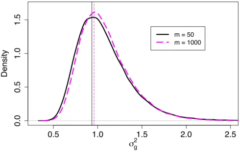
The fitted inverse gamma distributions of σ2g for m = 50 and 1000 are very similar, as shown as in Figure 2.5, where vertical lines indicate the modes. The middle three columns in Table 2.2
give the sample size and average power calculated by our ssizeRNA package. As shown in Table
2.2, the resulting sample sizes are all 13 whenm ranges from 50 to 1000. This is expected because Figure 2.5 indicates that the estimated distributions of σg2 are very close using different m values for this dataset.
0.5 1.0 1.5 2.0 2.5 0.0 0.5 1.0 1.5 σg2 Density m = 50 m = 1000
Figure 2.5 Fitted inverse gamma distributions ofσg2 for sample size m= 50 and 1000 for simulation 2.
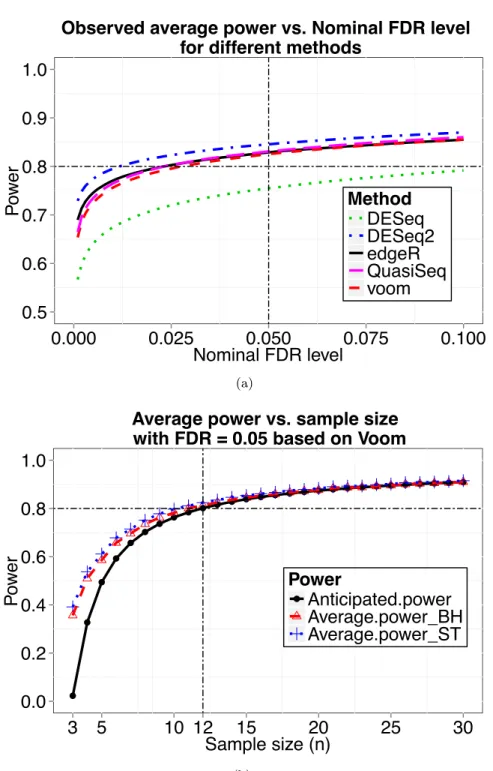
At n= 13, we checked the plots of average power vs. nominal FDR and true FDR vs. nominal FDR, and the results were similar to those obtained in simulation 1. More specifically, the desired power (0.8) was achieved, and FDR was controlled successfully. Actually, the desired power can be reached at sample size n= 11. Figure 2.6(a) gives the power curve calculated by our method based on hyperparameters estimated atm= 1000 together with observed power curves with FDR controlled by the Benjamini and Hochberg’s method and the q-value procedure, respectively. The anticipated power curve based on m= 1000 is close to the other two observed power curves.
The RnaSeqSampleSize R package (Zhao et al., 2015) could give an estimation of sample size and power by prior real data. They first use user-specified number of genes to estimate the gene read count and dispersion distribution, then sample size distribution and est power distribution
functions will be used to determine sample size and actual power. When we used the same real dataset as our simulation setting 2, the sample size calculated by their method was 7, with actual power 0.774, which did not reach the desired power 0.8. We also tried to apply their method using our simulated data (with different m), the resulting sample size is larger (n = 9). The power estimated by their method at n = 9 are shown in Table 2.2, and all their estimated power were actually smaller than 0.8. PROPERstarted from an estimation of mean and dispersion parameters, which is similar to our method. The sample size calculated by their method is 10, with power 0.804 based on DE detection methodedgeR. The comparison results of our proposed method and these three approaches are shown in the middle three columns of Table4.2. Still,PROPERis much more time-consuming than the other two methods.
2.3.3 Simulation 3. Gene-specific Mean and Dispersion with Different Fold Change
In this simulation, the setting is the same as the second simulation study, except that the fold changeδg was simulated from a log-normal distribution for differentially expressed genes. For
EE genes, both rg1j and rg2j were drawn from N B(λg, φg); for DE genes, rg1j were drawn from N B(λg, φg) andrg2j were drawn fromN B(λgδg, φg) or N B(λg/δg, φg) where
0.0 0.2 0.4 0.6 0.8 1.0 3 8 13 18 23 28 Sample size (n) P o w er Power Anticipated.power Observed.power_BH Observed.power_ST
Average power vs. sample size with FDR = 0.05 based on Voom
(a) 0.0 0.2 0.4 0.6 0.8 1.0 3 5 10 15 2022 25 30 35 40 Sample size (n) P o w er Power Anticipated.power Observed.power_BH Observed.power_ST
Average power vs. sample size with FDR = 0.05 based on Voom
(b)
Figure 2.6 Anticipated power curve calculated by ssizeRNA and observed power curves using voom and limma while FDR was controlled using either the Benjamini and Hochberg method (BH) or the q-value procedure by Storey and Tibshirani (ST) for simulation 2 (in (a)) and 3 (in (b)).
The last three columns in Table 2.2 give the sample size and power calculated by our method. As in simulation 2, varying the size of simulated data (m) did not result in different sample sizes. Anticipated and observed power curves are presented in Figure2.6(b), from which we notice that the three curves are almost indistinguishable after power reaches 60%. This more realistic simulation demonstrates that our proposed method provides accurate power and sample size.
We also applied RnaSeqSampleSize to this simulation setting. Since their method is based on minimum fold change, such results will be conservative due to the variability of fold change, especially as in this case, the minimum fold change is close to 1. When we used the 10th percentile of fold change of DE genes as the “minimum” fold change, the sample size calculated by their method was 74, which is still much larger than what we actually need, but the power calculated by their method based on the “minimum” fold change was less than the desired power 0.8. PROPER gave a result of sample size 19 with power 0.805 based on DE detection methodedgeR. The comparison results of our proposed method and these three approaches are shown in the last three columns of Table4.2.
Based on results from simulations, our proposed method and RnaSeqSampleSize provided an-swers much faster thanPROPER, and our proposed method andPROPER provided good sample size estimation. Overall, our proposed method worked the best while both accuracy and computa-tion time are considered.
2.3.4 Simulation 4. Real Data-based Simulation
Our method involves simulating data based on negative binomial distributions. To check the robustness of our method, we conducted a simulation based on a real RNA-seq dataset from Pickrell
et al.(2010), which was upon an RNA-seq experiment that sequenced 69 lymphoblastoid cell lines (LCL) derived from unrelated Nigerian individuals. We used the genes with minimum read counts across all individuals larger than 10, which results in 9154 genes. First, we estimated the mean and dispersion across all 69 individuals for each gene. Assume that fold change comes from a log-normal distribution as in simulation 3,
T able 2.3 Comparison of sample size calculation metho ds, including the prop osed metho d in this pap er, Zhao et al. (2015)’s approac h ( R naSe qSampleSize ) and W u et al. (2015)’s approac h ( PR O P ER ). Results determined b y our metho d w ere based on parameters estimated at m = 200. P o w e r w as ev aluated based on the vo om and limma pip eline for our metho d, while edgeR for R n aSe qSampleSize and PR OPE R . The computation time for eac h sim ulation w as calculated on a MacAir laptop with 1.3 GHz i7 CPU and 4GB RAM. Sim ulation 1 Sim u lation 2 Sim ulation 3 Metho d Sample P o w er Computation Sample P o w er Computation Sample P o w e r Computation size time size time size time Our Metho d 34 0.815 17.3 sec 13 0.823 16.8 sec 22 0.804 15.5 sec R n aSe qSampleSize 32 0.810 0.3 sec 9 0.765 54.6 sec 74 0.742 82.8 sec PR O P ER 25 0.806 6.5 hour 10 0.804 1.5 hour 19 0.805 3.5 h our
δg ∼log−normal(log(2),0.5log(2)),
the proportion of non-DE genes being 80%, to reach a desired power 0.8 while controlling FDR at 0.05, the sample size calculated by our method is 12 at m= 200.
To check whether desired power can be achieved at the calculated sample size, we simulated 100 datasets. For each simulation, we randomly picked 24 out of the 69 individuals and randomly assigned 12 individuals to the control group and the remaining 12 individuals to the treatment group. Consider all 9154 genes among the 24 individuals as EE since the samples were randomly selected from the same population. Then we randomly generated 20% of the 9154 genes to be DE, and their counts in the treatment group were multiplied by fold change δg which were drawn
from alog−normal(log(2),0.5log(2)) distribution. The scaled counts were rounded to the nearest integers. This strategy likely results in more realistic data because all counts come from real dataset and no distributional assumptions were imposed. The plot of average power vs. nominal FDR at n= 12 is shown in Figure2.7(a), where desired power (0.8) was achieved for most testing methods, including edgeR, DESeq2, QuasiSeq, voom and limma methods, when controlling FDR at 0.05 using q-value procedure. Figure2.7(b)gives the power calculated by our method based on hyperparameters estimated at m= 200. It also presents the observed average power curves when FDR was controlled by either the Benjamini and Hochberg’s method or the q-value procedure. The anticipated power curve based on m = 200 is close to the other two observed power curves. Hence, our proposed method also provides a reliable estimation of sample size and power in the most realistic simulation study.
2.4 Conclusions
In recent years, RNA-seq technology has become a major platform to study gene expression. With large sample size, RNA-seq experiments would be rather costly; while insufficient sample size may result in unreliable statistical inference. Thus sample size calculation is a crucial issue when designing an RNA-seq experiment. Although we could use a lot of simulations for each sample size
0.5
0.6
0.7
0.8
0.9
1.0
0.000
0.025
0.050
0.075
0.100
Nominal FDR level
P
o
w
er
Method
DESeq
DESeq2
edgeR
QuasiSeq
voom
Observed average power vs. Nominal FDR level
for different methods
(a)
0.0
0.2
0.4
0.6
0.8
1.0
3
5
10
12
15
20
25
30
Sample size (n)