Performance Evaluation of Cluster Validity Indices (CVIs) on Multi/Hyperspectral Remote Sensing Datasets

Article

Performance Evaluation of Cluster Validity Indices

(CVIs) on Multi/Hyperspectral Remote

Sensing Datasets

Huapeng Li1,*, Shuqing Zhang1, Xiaohui Ding1,2, Ce Zhang3and Patricia Dale4

1 _{Northeast Institute of Geography and Agroecology, Chinese Academy of Sciences, Changchun 130012,} China; [email protected] (S.Z.); [email protected] (X.D.)

2 _{University of Chinese Academy of Sciences, Beijing 100049, China}

3 _{Lancaster Environment Centre, Lancaster University, Lancaster LA1 4YQ, UK; [email protected]} 4 _{Environmental Futures Research Institute, School of Environment, Griffith University, Brisbane, QLD 4111,}

Australia; [email protected]

* Correspondence: [email protected]; Tel.: +86-431-8554-2230

Academic Editors: Guoqing Zhou, Qihao Weng and Prasad S. Thenkabail Received: 21 December 2015; Accepted: 21 March 2016; Published: 30 March 2016

Abstract:The number of clusters (i.e., the number of classes) for unsupervised classification has been recognized as an important part of remote sensing image clustering analysis. The number of classes is usually determined by cluster validity indices (CVIs). Although many CVIs have been proposed, few studies have compared and evaluated their effectiveness on remote sensing datasets. In this paper, the performance of 16 representative and commonly-used CVIs was comprehensively tested by applying the fuzzy c-means (FCM) algorithm to cluster nine types of remote sensing datasets, including multispectral (QuickBird, Landsat TM, Landsat ETM+, FLC1, and GaoFen-1) and hyperspectral datasets (Hyperion, HYDICE, ROSIS, and AVIRIS). The preliminary experimental results showed that most CVIs, including the commonly used DBI (Davies-Bouldin index) and XBI (Xie-Beni index), were not suitable for remote sensing images (especially for hyperspectral images) due to significant between-cluster overlaps; the only effective index for both multispectral and hyperspectral data sets was the WSJ index (WSJI). Such important conclusions can serve as a guideline for future remote sensing image clustering applications.

Keywords:cluster validity index; remote sensing; image clustering; cluster number of image

1. Introduction

Land use/cover data is crucial for diverse disciplines (e.g., ecology, geography, and climatology) since it serves as a basis for various “real world” applications [1–3]. Remote sensing technique have become the mainstream means to acquire land use/cover data, owing to its specific advantages, including synoptic views and cost-effectiveness [4,5]. Remote sensing image clustering, which utilizes only the statistical information inherent in the image without human interference, is one of the most widely used methods to produce land cover information [6,7]. It is also valued because of its high efficiency (i.e., it does not use training samples) [8].

The success of clustering (unsupervised classification) depends greatly on the proper determination of cluster number (i.e., the optimal number of classes) [9]: if the number of classes selected is less than the actual number, one or more separate classes would be merged into other classes; conversely, if larger, one or more homogeneous classes would be separated into different classes. The consequence is that the information contained in the raw data is incorrectly explored and used and the classification results will not be coincident with the “real” situation [10]. In this circumstance, the role

Remote Sens.2016,8, 295 2 of 22

of the cluster validity index (CVI), which is designed to detect the optimal cluster number for a given dataset, therefore, becomes critical [11].

Generally, a CVI is comprised of two indicators, namely compactness and separation. Compactness, which indicates the concentration of data points that belong to the same cluster, is usually measured by the distance between each data point and its cluster center [10]: the smaller the distance, the better the compactness of the cluster. Separation, which expresses the degree of isolation among clusters, is usually measured by the distance between cluster centroids: the larger the distance, the stronger the isolation of clusters [12]. Ideally, a dataset is partitioned with high compactness within each cluster and large separation between each pair of clusters. However, the two indicators are often mutually conflicting [13]; with increasing cluster number, the compactness becomes larger while the separation becomes smaller. Therefore, a good balance between the two indicators is required in the design of CVIs. To date, researchers from different disciplines have proposed a large number of CVIs for various types of applications.

In the remote sensing field, CVIs such as the Davies-Bouldin index (DBI) and the Xie-Beni index (XBI) have been widely used in image clustering applications. For example, DBI was employed to evaluate the fitness of candidate clustering by Bandyopadhyay and Maulik [9], and to guide satellite image clustering by Daset al.[14]; XBI was used to determine the optimal cluster number of IRS image by Maulik and Saha [15]; and was applied for multi-objective automatic image clustering [16,17]. However, in the absence of systematic and comprehensive evaluation of CVIs for remote sensing applications, CVIs are usually subjectively selected. This means that, without evaluation, they cannot necessarily be relied on. In fact, remote sensing data is well known for its complexity and uncertainty, with the specific characteristics as follows: (1) fuzzy and nonlinear class boundaries; (2) significant overlap among pixels from different classes (the overlap problem) [18]; and (3) high dimensionality and huge quantities of data. An appropriate CVI should, therefore, be designed taking account of these properties of remote sensing data.

To draw some general conclusions, although some efforts have been made to compare or evaluate the performance of CVIs in different environments [10,19–21], little attention has been paid to remote sensing data. Thus, the question remains as to how to select appropriate CVIs for remote sensing image clustering. Such a question can only be answered through an extensive evaluation of CVIs on various types of remote sensing data sets. However, to the best of our knowledge, few studies have addressed this issue. The objective of this paper is to fill that gap and identify one or several CVIs that are generally suitable for remote sensing datasets from a total of sixteen CVIs. The commonly used fuzzy c-means (FCM) and K-means algorithms were applied in this paper to cluster nine types of remote sensing datasets, including five types of multispectral and four types of hyperspectral images. This is of great significance since it can serve as a guideline for future remote sensing image clustering with diverse data types.

The remainder of this paper is organized as follows. In Section2, the clustering problem and the FCM and K-means algorithms are briefly outlined; the sixteen CVIs evaluated in this paper are reviewed and detailed in Section3; the experiments and results are provided in Section4; the results are analyzed and discussed in Section5; and conclusions are drawn in Section6.

2. The Clustering Problem

In this section, we briefly review the clustering problem and the classical fuzzy c-means algorithm. 2.1. The Clustering Problem

Clustering is widely used in many fields to derive information on distributions and patterns in raw data [11]. It aims at partitioning a given data set into groups (clusters) according to a predefined criteria (usually the Euclidean distance) [20]. LetX“ tx1,x2, . . . ,xNube a possible given dataset (with

Npoints), andKthe number of clusters (i.e., patterns) of the data. The purpose of clustering is to evolve a partition matrixUpXqof the data to determine a partitionC“ tC1,C2, . . . ,CKu, in which the

points in the same cluster are as close (i.e., have high similarity) as possible while those in different clusters are dispersed as far (i.e., have high dissimilarly) as possible. The partition matrix can be denoted asU“ rµi js, 1ďiďK, 1ďjď N, whereµijis the grade of membership of pointxjto cluster

Cipi“1, . . . ,Kq.

Clustering can be performed in two forms: crisp and fuzzy. In crisp clustering, any one point of the given dataset belongs to only one class of clusters, that isµij“ 1 ifxjPCi; otherwiseµij“0.

In fuzzy clustering, a point may belong to several or all classes with a certain grade of membership. In this case, the partition matrixUpXqis represented asU “ rµi js, whereµij P r0, 1s. It should be

noted that crisp clustering is a special version of fuzzy clustering in which the grade of membership of a point to a cluster is either 0 or 1. Once a fuzzy clustering structure is determined by a specific algorithm, each point of the given data will be assigned to the most likely cluster (i.e., with the largest grade of membership for that point). Through this process, the fuzzy clustering can be transformed into crisp clustering for real applications.

2.2. The Fuzzy C-Means Algorithm

The classical fuzzy c-means (FCM) algorithm proposed by Bezdek [22] has been successfully used in a wide domain of applications, such as agricultural engineering, image analysis, and target recognition, among others [20,23,24]. The objective of FCM is to evolve a set of cluster centers through minimizing the weighted within-cluster sum of squared error functionJm, which is defined as:

Jm“ N ÿ j“1 K ÿ i“1 pµijqm||xj´zi||2, 0ă N ÿ j“1 µijăN,iP t1, 2, . . . , Ku (1)

whereZ“ pz1,z2, . . . ,zKqis a group of cluster centers,ziPRd(dis the number of features included

in each point). || . . . || is a Euclidean norm measuring the similarity between a point and the corresponding cluster center. The weighting exponent m controls the fuzziness of the grade of membership. The partition matrixµijand the cluster center setZin the functionJmcan be calculated

using the following equations:

µij “ » – K ÿ i“1 p||xj´zi|| 2 ||xj´zk||2 q 1{pm´1qfi fl ´1 ,iP t1, 2, . . . ,Ku,jP t1, 2, . . . , Nu (2) and zi“ N ř j“1 pµijqmxj N ř j“1 pµijqm ,iP t1, 2, . . . , Ku (3)

The FCM algorithm iteratively searches the fuzzy partition matrix and the cluster centers with a greedy searching strategy, until either no more changes are found in the cluster centers or the differences between two successive cluster centers fall below a predefined threshold. Normally, the FCM algorithm consists of the following steps:

Step 1: Determine the number of clusterKand the weighting exponentm, initialize the cluster centersZpz1,z2, . . . ,zKqrandomly, and define a threshold of iteration terminationε.

Step 2: Update the fuzzy partition matrix using Equation (2). Step 3: Recalculate the cluster center setZnewusing Equation (3).

Step 4: If ||Znew´Z||ďε, stop the iteration and output the clustering result; otherwise, go to step 2.

Remote Sens.2016,8, 295 4 of 22

2.3. The K-Means Algorithm

The K-means algorithm is one of the most commonly used methods for unsupervised image classification [2]. Similar to FCM, the objective of K-means is to determine a set of cluster centers through minimizing the clustering metricM, which is defined as

M“ K ÿ i“1 ÿ x_jPC_i kxj´zi k (4)

whereCirepresents a cluster withzias its cluster center.

A greedy searching strategy is also employed in K-means to search for the optimal set of cluster centers, until a predefined termination condition is met. The main steps of the algorithm are as follows: Step 1: Determine the cluster numberKand the maximum iteration numberMax_iterto generate the initial cluster centers randomly.

Step 2: Assign pixelxjto clusterCiif ||xj´zi||ă||xj´zk||,kP t1, 2, . . . ,Ku, andi‰ k.

Step 3: Calculate new cluster center (znew_i ) for clusterCiasznew_i “

1 Ni

ř xjPCi

xj, whereNidenotes the

number of pixels in clusterCi.

Step 4: IfMax_iteris reached, terminate the cycle and output the clustering result; otherwise, go to Step 2.

3. Cluster Validity Indices (CVIs)

Broadly, current fuzzy CVIs (for fuzzy clustering) can be classified into two forms: one (called simple CVIs) only considers the fuzzy grades of membership to a class of the data (e.g., the partition coefficient), the other (called advanced CVIs) takes both fuzzy grads of membership and the geometrical properties (i.e.,the structure) of the original data into account (e.g., the well-known XBI) [10]. In fact, crisp CVIs (for crisp clustering) which only consider the geometrical properties of the original data (e.g., the well-known DBI) are special versions of advanced CVIs, and can also be used in fuzzy image clustering analysis [12]. In this study, a total of 16 representative and commonly used CVIs of different forms were chosen for evaluation, including three simple CVIs, and thirteen advanced CVIs.

It is noteworthy that some CVIs (e.g., XBI) indicate the optimal cluster number of data by using the maximum value, while the others use the minimum value. For convenience, we subsequently denote the former (the larger, the better CVI) as CVI+_{, and the latter (the lower, the better CVI) as CVI}´_. 3.1. Simple CVIs

(1) The partition coefficient (PC+_{) [25] evaluates the compactness by using the averaged strength} of belongingness of data, and is defined as:

PCpKq “ 1 N K ÿ i“1 N ÿ j“1 µ2_ij (5)

(2) The partition entropy (PE´_{) is formed based upon the logarithmic form ofPC[22], and is} defined as: PEpKq “ ´1 N K ÿ i“1 N ÿ j“1 µijlog2puijq (6)

(3) The modification ofPC(MPC+) [26] is designed to reduce the monotonic tendency ofPCand PE. The index is defined as:

MPCpKq “1´ K

3.2. Advanced CVIs

(1) The Davies-Bouldin Index (DBI´_{) [27] estimates the ratio of within-cluster compactness to} between-cluster separation, which is defined as:

DBIpKq “ 1 K K ÿ i“1 maxt Si`Sk ||zi´zk||2 u,i‰k, (8) whereSi“ 1 Ni ř xjPCi||xj´zi|| 2_,N

idenotes the number of data points in theith cluster (Ci).

(2) The Dunn Index (DI+) [28] evaluates a clustering by taking the minimum distance between-cluster as separation and the maximum distance between each pair of within-cluster points as compactness. The original index is defined as [28]:

DunnpKq “ min 1ďpďK ¨ ˝ min s`1ďqďK´1p dispCp,Cqq max 1ďiďKdiapCiq q ˛ ‚, (9)

wheredispCp,Cqqrefers to the distance between thepth andqth clusters, is calculated asdispCp,Cqq “

min

x_jPCp,xlPCq

p||xj´xl||q;diapCiqdenotes the maximum distance between any pair of within-cluster

points, which is measured asdiapCiq “ max xj,xlPCi

p||xj´xl||q.

(3) The Calinski-Harabasz Index (CHI+) [29] is a ratio-type index in which compactness is measured by the distance (WK) between each within-cluster point to its centroid, and separation

is based on the distance (BK) between each centroid to the global centroid (z),i.e.,:

CH IpKq “ BK K´1{ WK N´K, (10) whereBK“ K ř i“1 Ni||zi´z||2,WK“ K ř i“1 ř xjPCi ||xj´zi||2.

(4) The Fukuyama and Sugeno Index (FSI´_{) [30] is designed to measure the discrepancy between} fuzzy compactness and fuzzy separation,i.e.,:

FSIpKq “ K ÿ i“1 N ÿ j“1 um_ij||xj´zi||2´ K ÿ i“1 N ÿ j“1 um_ij||zi´ ´ z|| 2 (11)

(5) The Xie and Beni Index (XBI´_{) [31] is also a ratio-type index, which measures the average} within-cluster fuzzy compactness against the minimum between-cluster separation,i.e.,:

XBIpKq “ K ř i“1 N ř j“1 µ2_ij||xj´zi||2 N¨min i‰kt||zi´zk|| 2 u (12)

(6) The Kwon Index (KI´_{) [32] aims to overcome the shortcoming of XBI that decreases} monotonically when the cluster number approaches the actual cluster number of data. Here, a penalty function was introduced to the numerator of XBI,i.e.,:

KIpKq “ K ř i“1 N ř j“1 µ2_ij||xj´zi||2` 1 K K ř i“1 ||zi´ ´ z|| 2 min i‰kt||zi´zk|| 2_u (13)

Remote Sens.2016,8, 295 6 of 22

(7) The Tang Index (TI´_{) [33] also introduced a similar penalty function to the numerator} of XBI,i.e.: T IpKq “ K ř i“1 N ř j“1 µ2_ij||xj´zi||2` 1 KpK´1q K ř i“1 K ř k“1 k‰i ||zi´zk||2 min i‰k||zi´zk|| 2<sub>`1{K</sub> (14)

(8) The SC Index (SCI+) [34] measures the fuzzy compactness/separation ratio of clustering by using the difference between two functions,SC1andSC2,i.e.,:

SCIpKq “SC1pKq ´SC2pKq, (15)

whereSC1(Equation (16)) evaluates the compactness/separation ratio by considering the grades of membership and the original data: the larger theSC1, the better the clustering:

SC1pKq “ p1 K K ř i“1 ||zi´z||q K ř i“1 p N ř j“1 µm_ij||xj´zi||2{ N ř j“1 µijq , (16)

whileSC2(Equation (17)) measures the ratio by using the grades of membership only: the smaller the SC2, the better the clustering:

SC2pKq “ K´1 ř i“1 K ř k“i`1 p N ř j“1 pminpµij,µkjq2q{njkq p N ř j“1 max 1ďiďKµ 2 ijq{p N ř j“1 max 1ďiďKµijq (17) wherenjk “ N ř j“1 minpµij,µkjq.

(9) The Compose Within and Between scattering Index (CWBI´_{) [19] assesses the average} compactness and separation of fuzzy clustering by using the sum of two functions,i.e.,:

CWBIpKq “αScatpKq `DispKq, (18)

whereαis a weighing factor which equalsDispKmaxq, theDispKqwith the maximum cluster number; andScatpKqrefers to the average scattering (i.e., compactness) forKclusters, which is defined as:

ScatpKq “ 1 K K ř i“1 ||σpziq|| ||σpXq|| , (19)

where ||x|| “ pxT¨xq1{2; σpXq denotes the variance of data, which is defined as σpXq “ 1

N

N ř j“1

pxj´zq2; σpziq denotes the fuzzy variation of cluster i, which is defined as σpziq “

1 N N ř j“1 µijpxj´ziq2.

The smaller the value ofScatpKq, the better the compactness of the clustering.

The distance functionDispKqmeasuring the separation between clusters is defined as:

DispKq “ Dmax Dmin K ÿ i“1 p K ÿ k“1 ||zi´zk||q ´1 , (20)

whereDmax“maxt||zi´zk||u,Dmin“mint||zi´zk||u,i,kP{2, 3, . . . K}.

The smaller the value ofDispKq, the better the separation of clusters.

(10) The WSJ Index (WSJI´_{) [13], inspired by the CWBI, also uses a linear combination of averaged} fuzzy compactness and separation to measure clustering, which is defined as:

WSJ IpKq “ScatpKq ` SeppKq

SeppKmaxq (21)

where ScatpKq is given by Equation (19); SeppKq denotes the between-cluster separation, which is defined as SeppKq “ D 2 max D_min2 K ř i“1 p K ř k“1 ||zi´zk||2q ´1

, where Dmax “ maxt||zi´zk||u, Dmin “ mint||zi´zk||u;SeppKmaxqrefers to theSeppKqwith the maximum cluster number.

(11) The PBMF index (PBMFI+) [20] estimates within-cluster compactness and large separation between clusters of fuzzy clustering,i.e.,:

PBMFIpKq “ max i‰k t||zi´zk||u ˆ N ř j“1 µj1||xi´z1|| K K ř i“1 N ř j“1 µm_ij||xj´zi|| . (22)

(12) The SVF index (SVFI+) [35] emphasizes on low within-cluster variation (i.e., high compactness) and large separation between clusters,i.e.,:

SVFIpKq “ K ř i“1 min i‰k||zi´zk|| K ř i“1 maxxjPCiµ m ij||xj´zi|| . (23)

(13) The WL Index (WLI´_{) [12] measures both within-cluster compactness and between-cluster} separation of fuzzy clustering. Specifically, it takes both the minimum and the median distances between clusters as separation, which retains the clusters whose centroids are close to each other. The index is defined as:

W LIpKq “ W Ln 2W Ld

(24) where W Ln denotes the fuzzy compactness of clusters, which is defined as W Ln “

K ř i“1 p N ř j“1 µ2_ij||xj´zi||2 N ř j“1 µij

q;W Ldrefers to the separation between clusters, which is defined asW Ld “

1

2pmini‰kt||zi´zk||

2

u `median

i‰k t||zi´zk||

2_{uq, where min}

i‰kt||zi´zk||

2

u and mediant||zi´zk||2u

denote, respectively, the minimum distance and median distance between any pair of clusters. 4. Experiments and Results

In this section, the performance of the 16 CVIs introduced in Section3was evaluated using five types of multispectral, and four types of hyperspectral, remote sensing datasets (detailed below). For image clustering, the FCM and K-means algorithms were utilized here. The operational parameters in FCM were designated in line with previous studies [13]: threshold of iteration terminationε“ e´5, weighting exponentm“2, and the maximum iteration numberMax_iter“500; while the operational parameters in K-means as: the pixel change threshold = 0%, and the maximum iteration number Max_iter“500. For each of the images, the two algorithms were implemented with cluster number

Remote Sens.2016,8, 295 8 of 22

K “2, 3, . . . , 10, respectively. To overcome the shortcoming of the two algorithms that often trap on local optima, depending on the initial solutions [36], each implementation of the clustering was repeated five times and the best clustering result (with the minimum value ofJm(Equation (1)) orM

(Equation (4)) was retained for CVIs evaluation. 4.1. Datasets

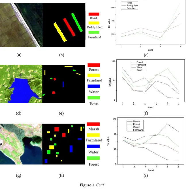
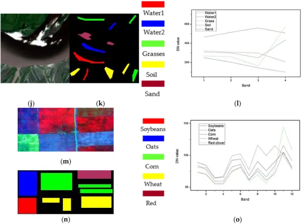
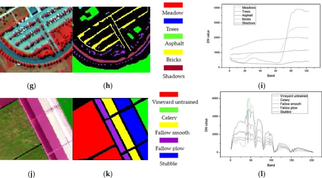
The five multispectral data sets include QuickBird [37], Landsat TM, Landsat ETM+, GaoFen-1 [38], and FLC1 [39]. Their true/false color maps, the corresponding ground reference maps and the spectral curves of land use/cover classes were shown in Figure1. The four hyperspectral datasets include Hyperion [40], HYDICE [41], ROSIS [42] and AVIRIS [43]. Their false color maps, ground reference maps and spectral curves of land cover/use classes were presented in Figure2. The basic information on the remote sensing datasets employed in our experiments was detailed in Table1.

Remote Sens. 2016, 8, 295 8 of 23 d n

WL

WL

K

WLI

2

)

(

=

₍₂₄₎

where

WL

n denotes the fuzzy compactness of clusters, which is defined as







= = = − = K i N j ij N j i j ij n z x WL 1 1 1 2 2 ) ( μ μ

;

WL

d refers to the separation between clusters, which is defined as

})

{

}

{

min

(

2

1

2 2 k i k i k i k i d

z

z

median

z

z

WL

=

−

+

−

≠ ≠ , where

min

{

}

2 k i k i_≠

z

−

z

and

}

{

z

_i

z

_k 2

median

−

denote, respectively, the minimum distance and median distance between any

pair of clusters.

4. Experiments and Results

In this section, the performance of the 16 CVIs introduced in Section 3 was evaluated using five types of multispectral, and four types of hyperspectral, remote sensing datasets (detailed below). For image clustering, the FCM and K-means algorithms were utilized here. The operational parameters in FCM were designated in line with previous studies [13]: threshold of iteration termination

e

=

ε

− 5, weighting exponent

m

=

2

, and the maximum iteration number

Max

_

iter

=

500

; while the operational parameters in K-means as: the pixel change threshold = 0%, and the maximum iteration number

Max

_

iter

=

500

. For each of the images, the two algorithms were implemented with cluster number

K

=

2

,

3

,

...,

10

, respectively. To overcome the shortcoming of the two algorithms that often trap on local optima, depending on the initial solutions [36], each implementation of the clustering was repeated five times and the best clustering result (with the minimum value of

J

m (Equation (1)) or

M

(Equation (4)) was retained for CVIs

evaluation.

4.1. Datasets

The five multispectral data sets include QuickBird [37], Landsat TM, Landsat ETM+, GaoFen-1 [38], and FLC1 [39]. Their true/false color maps, the corresponding ground reference maps and the spectral curves of land use/cover classes were shown in Figure 1. The four hyperspectral datasets include Hyperion [40], HYDICE [41], ROSIS [42] and AVIRIS [43]. Their false color maps, ground reference maps and spectral curves of land cover/use classes were presented in Figure 2. The basic information on the remote sensing datasets employed in our experiments was detailed in Table 1.

(a) (b) (c) Figure 1.Cont. Remote Sens. 2016, 8, 295 9 of 23 (d) (e) (f) (g) (h) (i) (j) (k) (l) (m) (n) (o)

Figure 1. The multispectral images. (a–c) the true/false color map, the ground reference map and the corresponding spectral curves of ground truth classes of QuickBird datasets; (d–f) the corresponding maps of Landsat TM datasets; (g–i) the corresponding maps of Landsat ETM+ datasets; (j–l) the corresponding maps of GaoFen-1 datasets; (m–o) the corresponding maps of FLC1 datasets. (a) True color map; (b) false color map (7, 5, 3); (c) false color map (7, 5, 3); (d) true color map; and (e) false color map (bands 12, 9, and 1).

Remote Sens.2016,8, 295 9 of 22 (d) (e) (f) (g) (h) (i) (j) (k) (l) (m) (n) (o)

Figure 1. The multispectral images. (a–c) the true/false color map, the ground reference map and the corresponding spectral curves of ground truth classes of QuickBird datasets; (d–f) the corresponding maps of Landsat TM datasets; (g–i) the corresponding maps of Landsat ETM+ datasets; (j–l) the corresponding maps of GaoFen-1 datasets; (m–o) the corresponding maps of FLC1 datasets. (a) True color map; (b) false color map (7, 5, 3); (c) false color map (7, 5, 3); (d) true color map; and (e) false color map (bands 12, 9, and 1).

Figure 1.The multispectral images. (a–c) the true/false color map, the ground reference map and the corresponding spectral curves of ground truth classes of QuickBird datasets; (d–f) the corresponding maps of Landsat TM datasets; (g–i) the corresponding maps of Landsat ETM+ datasets; (j–l) the corresponding maps of GaoFen-1 datasets; (m–o) the corresponding maps of FLC1 datasets. (a) True color map; (b) false color map (7, 5, 3); (c) false color map (7, 5, 3); (d) true color map; and (e) false color map (bands 12, 9, and 1).

Remote Sens. 2016, 8, x 10 of 23

(a) (b) (c)

(d) (e) (f)

(g) (h) (i)

(j) (k) (l)

Figure 2. The hyperspectral images. (a–c) the false color (FC) map, the corresponding ground reference map and the corresponding spectral curves of ground truth classes of Hyperion data sets; (d–f) the corresponding maps of HYDICE datasets; (g–i) the corresponding maps of ROSIS datasets; (j–l) the corresponding maps of AVIRIS datasets. (a) FC map (bands 93, 60, 10); (b) FC map (bands 120, 90, 10); (c) FC map (bands 90, 60, 10); and (d) FC map (bands 111, 90, 12).

Table 1. Basic information of the remote sensing data sets.

D S Y L R B W S GT

QuickBird Multi-spectral camera 2005

Yalvhe farm,

China 2.4 4 0.45–0.90 100 × 100

Road, paddy field, and farmland Landsat TM Thematic mapper 2005 JingYuetan reservoir, China 30 6 0.45–2.35 296 × 295 Forest, farmland, water, and town Landsat ETM+ Enhanced thematic mapper 2001 Zhalong reserve, China 30 6 0.45–2.35 150 × 139

Marsh, forest, water, and farmland

Gaofen-1 Wide filed imager 2015

Sanjiang Plain,

China 16 4 0.45–0.89 200 × 200

Water1, water2, grass, soil, and sand

Remote Sens.2016,8, 295 10 of 22 Remote Sens. 2016, 8, x 10 of 23 (a) (b) (c) (d) (e) (f) (g) (h) (i) (j) (k) (l)

Figure 2. The hyperspectral images. (a–c) the false color (FC) map, the corresponding ground reference map and the corresponding spectral curves of ground truth classes of Hyperion data sets; (d–f) the corresponding maps of HYDICE datasets; (g–i) the corresponding maps of ROSIS datasets; (j–l) the corresponding maps of AVIRIS datasets. (a) FC map (bands 93, 60, 10); (b) FC map (bands 120, 90, 10); (c) FC map (bands 90, 60, 10); and (d) FC map (bands 111, 90, 12).

Table 1. Basic information of the remote sensing data sets.

D S Y L R B W S GT

QuickBird Multi-spectral camera 2005

Yalvhe farm,

China 2.4 4 0.45–0.90 100 × 100

Road, paddy field, and farmland Landsat TM Thematic mapper 2005 JingYuetan reservoir, China 30 6 0.45–2.35 296 × 295 Forest, farmland, water, and town Landsat ETM+ Enhanced thematic mapper 2001 Zhalong reserve, China 30 6 0.45–2.35 150 × 139

Marsh, forest, water, and farmland

Gaofen-1 Wide filed

imager 2015

Sanjiang Plain,

China 16 4 0.45–0.89 200 × 200

Water1, water2, grass, soil, and sand

Figure 2.The hyperspectral images. (a–c) the false color (FC) map, the corresponding ground reference map and the corresponding spectral curves of ground truth classes of Hyperion data sets; (d–f) the corresponding maps of HYDICE datasets; (g–i) the corresponding maps of ROSIS datasets; (j–l) the corresponding maps of AVIRIS datasets. (a) FC map (bands 93, 60, 10); (b) FC map (bands 120, 90, 10); (c) FC map (bands 90, 60, 10); and (d) FC map (bands 111, 90, 12).

Table 1.Basic information of the remote sensing data sets.

D S Y L R B W S GT

QuickBird Multi-spectral_camera 2005 Yalvhe farm,_China 2.4 4 0.45–0.90 100ˆ100 Road, paddy field, and farmland Landsat TM Thematic_mapper 2005 JingYuetanreservoir,

China 30 6 0.45–2.35 296

ˆ295 _{water, and town}Forest, farmland,

Landsat ETM+ Enhanced thematic mapper 2001 Zhalong reserve, China 30 6 0.45–2.35 150

ˆ139 Marsh, forest, water,_{and farmland}

Gaofen-1 Wide filed_imager 2015 Sanjiang

Plain, China 16 4 0.45–0.89 200ˆ200

Water1, water2, grass, soil, and sand FLC1 M7 scanner 1966 Tippecanoe_{County, US} 30 12 0.40–1.00 84ˆ183 wheat andSoybeans, oats, corn,

red clover Hyperion Hyperion 2001 OkavangoDelta,

Botswana

30 145 0.40–2.50 126ˆ146 Woodland, islandinterior, water and floodplain grasses HYDICE HYDICE 1995 Washington_{DC, US} 2 191 0.40–2.40 126ˆ82 Roads, trees, trail_{and grass}

ROSIS ROSIS 2001 Universityof Pavia, Italy

1.3 103 0.43–0.86 125ˆ148 Meadows, trees,asphalt, bricks and shadows

AVIRIS AVIRIS 1998 _{Valley, USA}Salinas 3.7 204 0.41–2.45 117ˆ143

Vineyard untrained, celery, fallow smooth, fallow plow and stubble

Note: D, datasets; S, sensor; Y, year; L, location; R, resolution (m); B, number of bands; W, spectral wavelength (µm); S, size of image (pixel by pixels); GT, ground truth classes.

4.2. Results

The nine types of images were clustered by FCM and K-means algorithms respectively, and each clustering result was evaluated using the corresponding ground-truth data (Figures1and2). Table2 shows the classification accuracies of the images achieved by the two algorithms. Similarly, both FCM and K-means generated good classification results, with the overall accuracy greater than 90%

for seven images. However, considering the length limitation of the paper, the clustering results by K-means and the corresponding cluster validity result for each image were not presented in as much detail as those by FCM, but were summarized at the end of the results.

Table 2. Classification accuracies of the remote sensing images acquired by FCM and

K-means algorithms.

Datasets K# Overall Accuracies (%) Kappa Coefficient

FCM K-Means FCM K-Means QuickBird 3 96.06 96.10 0.9354 0.9361 Landsat TM 4 95.78 95.27 0.9433 0.9363 Landsat ETM+ 4 94.41 96.30 0.9253 0.9565 Gaofen-1 5 98.34 98.79 0.9791 0.9848 FLC1 5 83.10 84.48 0.7847 0.8016 Hyperion 4 87.09 86.79 0.8260 0.8219 HYDICE 4 94.88 96.00 0.9238 0.9403 ROSIS 5 93.85 93.25 0.9129 0.9044 AVIRIS 5 99.63 99.63 0.9946 0.9946

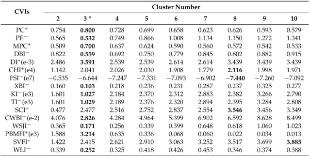
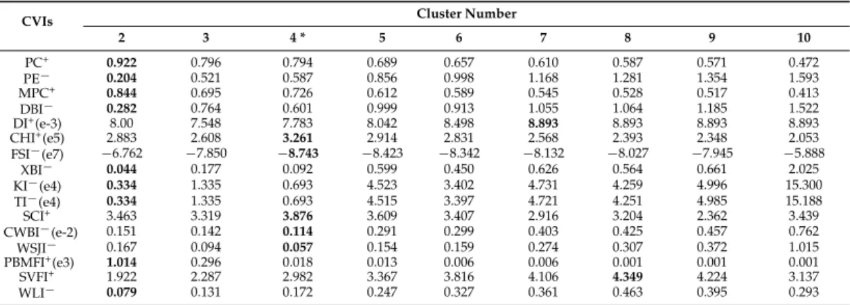
Tables3–11illustrated the variations of the 16 CVIs with the number of clusters ranging from two to 10 by FCM for each image. The optimal cluster numbers of each image are indicated by the CVIs, shown in bold font. The clustering results of multispectral and hyperspectral datasets by FCM, respectively, are illustrated in Figures3and4. Note that only four clustering results for each image are presented, including the optimal one (underlined), one or two close to the optimal, and those indicated by many CVIs (usually larger than 4) (bold). For example, Figure3e–h illustrates the clustering results of Landsat TM image, in which the optimal clustering (Figure3g) is underlined, the two near-optimal clustering results (Figure3f,h) and the obviously-incorrect clustering indicated by many CVIs (Figure3e) are also presented.

Table 3.Variations of the 16 CVIs with cluster numbers ranging from 2 to 10 for the QuickBird image.

CVIs Cluster Number

2 3 * 4 5 6 7 8 9 10 PC+ 0.754 0.800 0.728 0.699 0.658 0.623 0.626 0.593 0.579 PE´ _{0.565 0.532 0.749 0.866 1.008 1.134 1.150 1.272 1.341} MPC+ 0.509 0.700 0.637 0.624 0.590 0.560 0.572 0.542 0.533 DBI´ _{0.822 0.559 0.692 0.750 0.779 0.845 0.802 0.882 0.915} DI+(e-3) 2.486 3.591 2.539 2.539 2.614 2.614 3.439 3.439 3.439 CHI+(e4) 1.142 2.041 2.026 2.030 1.908 1.779 2.116 1.998 1.971 FSI´_{(e7) ´0.535 ´6.644 ´7.247 ´7.331 ´7.093 ´6.902 ´7.440 ´7.260 ´7.092} XBI´ _{0.160 0.103 0.218 0.236 0.231 0.287 0.237 0.325 0.277} KI´_{(e3) 1.601 1.027 2.184 2.370 2.312 2.883 2.382 3.266 2.790} TI´_{(e3) 1.601 1.029 2.189 2.376 2.320 2.894 2.395 3.284 2.808} SCI+ 0.477 2.477 2.516 2.752 2.837 2.554 3.546 3.456 3.349 CWBI´_{(e-2) 4.076 2.826 4.284 4.964 5.399 6.902 6.592 8.628 8.499} WSJI´ _{0.365 0.171 0.256 0.339 0.399 0.648 0.618 1.060 1.023} PBMFI+(e3) 1.588 3.214 0.635 0.336 0.068 0.060 0.022 0.034 0.013 SVFI+ 1.422 2.415 2.621 2.910 3.063 3.252 3.517 3.699 3.885 WLI´ _{0.339 0.252 0.325 0.418 0.426 0.453 0.346 0.374 0.388}

Note: *denotes the actual cluster number of the image; figures in bold face denote the optimal cluster numbers of the image identified by the CVIs; the data in the brackets of the first column is a multiplying factor (e.g., e-3 followed DI+_{) of the corresponding line.}

Remote Sens.2016,8, 295 12 of 22 Remote Sens. 2016, 8, 295 12 of 23 (a) (b) (c) (d) (e) (f) (g) (h) (i) (j) (k) (l) (m) (n) (o) (p) (q) (r) (s) (t)

Figure 3. Clustering results of the multispectral images (each color represents a cluster). (a) QuickBird,

K = 2; (b) QuickBird, K = 3; (c) QuickBird, K = 4; (d) QuickBird, K = 5; (e) Landsat TM, K = 2; (f) Landsat TM, K = 3; (g) Landsat TM, K = 4; (h) Landsat TM, K = 5; (i) Landsat ETM+, K = 2; (j) Landsat ETM+,

K = 3; (k) Landsat ETM+, K = 4; (l) Landsat ETM+, K = 5; (m) GaoFen-1, K = 2; (n) GaoFen-1, K = 4; (o) GaoFen-1, K = 5; (p)GaoFen-1, K = 6; (q) FLC1, K = 2; (r) FLC1, K = 3; (s) FLC1, K = 5; and (t) FLC1, K

= 6.

Figure 3.Clustering results of the multispectral images (each color represents a cluster). (a) QuickBird, K = 2; (b) QuickBird,K= 3; (c) QuickBird, K = 4; (d) QuickBird, K= 5; (e)Landsat TM, K= 2; (f) Landsat TM, K= 3; (g) Landsat TM,K= 4; (h) Landsat TM, K = 5; (i)Landsat ETM+, K = 2; (j) Landsat ETM+,K= 3; (k) Landsat ETM+,K= 4; (l) Landsat ETM+,K= 5; (m)GaoFen-1, K= 2; (n) GaoFen-1,K = 4; (o) GaoFen-1,K= 5; (p) GaoFen-1,K = 6; (q)FLC1, K= 2; (r)FLC1, K= 3; (s) FLC1,K= 5; and (t) FLC1,K= 6.

(a) (b) (c) (d)

(e) (f) (g) (h)

(i) (j) (k) (l)

(m) (n) (o) (p)

Figure 4. Clustering results of the hyperspectral images by FCM (each color represents a cluster). (a) Hyperion, K = 2; (b) Hyperion, K = 3; (c) Hyperion, K = 4; (d) Hyperion, K = 5; (e) HYDICE, K = 3; (f) HYDICE, K = 4; (g) HYDICE, K = 5; (h) HYDICE, K = 6; (i) ROSIS, K = 3; (j) ROSIS, K = 4; (k) ROSIS, K

= 5; (l) ROSIS, K = 6; (m) AVIRIS, K = 3; (n) AVIRIS, K = 4; (o) AVIRIS, K = 5; and (p) AVIRIS, K = 6.

Table 3. Variations of the 16 CVIs with cluster numbers ranging from 2 to 10 for the QuickBird image.

CVIs Cluster Number

2 3 * 4 5 6 7 8 9 10 PC+ _{0.754 0.800 0.728 0.699 0.658 0.623 0.626 0.593 0.579} PE− _{0.565 0.532 0.749 0.866 1.008 1.134 1.150 1.272 1.341} MPC+ _{0.509 0.700 0.637 0.624 0.590 0.560 0.572 0.542 0.533} DBI− _{0.822 0.559 0.692 0.750 0.779 0.845 0.802 0.882 0.915} DI+_{(e-3) 2.486 3.591 2.539 2.539 2.614 2.614 3.439 3.439 3.439} CHI+_{(e4) 1.142 2.041 2.026 2.030 1.908 1.779 2.116 1.998 1.971} FSI−_{(e7) −0.535 −6.644 −7.247 −7.331 −7.093 −6.902 −7.440 −7.260 −7.092} XBI− _{0.160 0.103 0.218 0.236 0.231 0.287 0.237 0.325 0.277} KI−_{(e3) 1.601 1.027 2.184 2.370 2.312 2.883 2.382 3.266 2.790} TI−_{(e3) 1.601 1.029 2.189 2.376 2.320 2.894 2.395 3.284 2.808} SCI+ _{0.477 2.477 2.516 2.752 2.837 2.554 3.546 3.456 3.349} CWBI−_{(e-2) 4.076 2.826 4.284 4.964 5.399 6.902 6.592 8.628 8.499} WSJI− _{0.365 0.171 0.256 0.339 0.399 0.648 0.618 1.060 1.023}

Figure 4. Clustering results of the hyperspectral images by FCM (each color represents a cluster). (a)Hyperion,K= 2; (b) Hyperion, K = 3; (c) Hyperion,K= 4; (d) Hyperion, K = 5; (e)HYDICE,

K= 3; (f) HYDICE,K= 4; (g) HYDICE,K= 5; (h) HYDICE,K= 6; (i)ROSIS,K= 3; (j) ROSIS,K= 4; (k) ROSIS,K= 5; (l) ROSIS,K = 6; (m) AVIRIS,K = 3; (n)AVIRIS, K= 4; (o) AVIRIS,K= 5; and (p) AVIRIS,K= 6.

Table 4.Variations of the 16 CVIs with cluster numbers ranging from 2 to 10 for the Landsat TM image.

CVIs Cluster Number

2 3 4 * 5 6 7 8 9 10 PC+ _{0.922 0.796 0.794 0.689 0.657 0.610 0.587 0.571 0.472} PE´ _{0.204 0.521 0.587 0.856 0.998 1.168 1.281 1.354 1.593} MPC+ _{0.844 0.695 0.726 0.612 0.589 0.545 0.528 0.517 0.413} DBI´ _{0.282 0.764 0.601 0.999 0.913 1.055 1.064 1.185 1.522} DI+_{(e-3) 8.00 7.548 7.783 8.042 8.498 8.893 8.893 8.893 8.893} CHI+_{(e5) 2.883 2.608 3.261 2.914 2.831 2.568 2.393 2.348 2.053} FSI´_{(e7) ´6.762 ´7.850 ´8.743 ´8.423 ´8.342 ´8.132 ´8.027 ´7.945 ´5.888} XBI´ _{0.044 0.177 0.092 0.599 0.450 0.626 0.564 0.661 2.025} KI´_{(e4) 0.334 1.335 0.693 4.523 3.402 4.731 4.259 4.996 15.300} TI´_{(e4) 0.334 1.335 0.693 4.515 3.397 4.721 4.251 4.985 15.188} SCI+ _{3.463 3.319 3.876 3.609 3.407 2.916 3.204 2.362 3.439} CWBI´_{(e-2) 0.151 0.142 0.114 0.291 0.299 0.403 0.425 0.457 0.762} WSJI´ _{0.167 0.094 0.057 0.154 0.159 0.274 0.307 0.372 1.015} PBMFI+_{(e3) 1.014 0.296 0.018 0.013 0.006 0.006 0.001 0.001 0.001} SVFI+ _{1.922 2.287 2.982 3.367 3.816 4.106 4.349 4.224 3.137} WLI´ 0.079 0.131 0.172 0.247 0.327 0.361 0.463 0.395 0.293

Remote Sens.2016,8, 295 14 of 22

Table 5.Variations of the 16 CVIs with cluster numbers ranging from 2 to 10 for the ETM+ image.

CVIs Cluster Number

2 3 4 * 5 6 7 8 9 10 PC+ _{0.404 0.812 0.760 0.725 0.703 0.663 0.628 0.617 0.593} PE´ _{0.284 0.503 0.673 0.802 0.877 1.012 1.144 1.204 1.300} MPC+ _{0.775 0.717 0.680 0.656 0.644 0.607 0.575 0.569 0.548} DBI´ _{0.404 0.603 0.674 0.731 0.745 0.861 0.952 0.937 1.055} DI+_{(e-3) 5.803 7.595 8.256 8.889 8.889 0.104 0.107 0.107 0.114} CHI+_{(e5) 0.818 0.909 0.929 0.929 0.896 0.893 0.847 0.847 0.822} FSI´_{(e8) ´0.409 ´0.483 ´0.477 ´0.461 ´0.461 ´0.439 ´0.426 ´0.422 ´0.413} XBI´ _{0.047 0.090 0.117 0.169 0.183 0.202 0.234 0.216 0.293} KI´_{(e4) 0.100 0.188 0.244 0.352 0.382 0.421 0.489 0.452 0.613} TI´_{(e4) 0.099 0.189 0.244 0.353 0.383 0.422 0.490 0.454 0.615} SCI+ _{2.463 3.259 3.388 3.723 4.715 5.137 4.922 4.779 4.884} CWBI´ _{0.054 0.059 0.076 0.104 0.112 0.133 0.164 0.174 0.226} WSJI´ _{0.162 0.351 0.126 0.214 0.248 0.348 0.515 0.601 1.012} PBMFI+_{(e3) 1.058 0.156 0.085 0.088 0.004 0.005 0.002 0.014 0.003} SVFI+ _{2.173 2.413 3.027 0.760 3.155 3.339 3.521 3.607 3.648} WLI´ _{0.093 0.174 0.307 0.265 0.244 0.229 0.259 0.208 0.279}

Note:*denotes the actual cluster number of the image.

Table 6.Variations of the 16 CVIs with cluster numbers ranging from 2 to 10 for the GaoFen-1 image.

CVIs Cluster Number

2 3 4 5 * 6 7 8 9 10 PC+ _{0.850 0.751 0.764 0.779 0.735 0.710 0.688 0.669 0.645} PE´ _{0.374 0.643 0.663 0.658 1.183 0.900 0.978 1.056 1.140} MPC+ _{0.700 0.627 0.620 0.724 0.682 0.662 0.643 0.628 0.606} DBI´ _{0.587 0.832 0.767 0.536 0.701 0.740 0.789 0.803 0.896} DI+_{(e-3) 4.715 1.478 1.470 2.298 2.348 2.688 3.028 2.860 2.965} CHI+_{(e5) 0.764 0.656 0.681 1.314 1.185 1.262 1.270 1.257 1.197} FSI´_{(e9) ´0.662 ´1.038 ´1.253 ´1.603 ´1.571 ´1.539 ´1.519 ´1.490 ´1.462} XBI´ _{0.100 0.135 0.136 0.077 0.198 0.158 0.140 0.154 0.285} KI´_{(e4) 0.399 0.541 0.546 0.309 0.791 0.634 0.560 0.617 1.141} TI´_{(e4) 0.399 0.541 0.546 0.309 0.792 0.635 0.561 0.618 1.141} SCI+ _{1.031 1.156 1.364 4.658 3.899 4.468 4.470 4.333 3.992} CWBI´_{(e-3) 0.147 0.137 0.144 0.139 0.240 0.264 0.268 0.311 0.445} WSJI´ _{0.226 0.934 0.128 0.114 0.282 0.348 0.362 0.487 1.015} PBMFI+_{(e4) 1.049 0.243 0.075 0.053 0.063 0.019 0.011 0.040 0.056} SVFI+ _{2.315 2.610 3.027 3.707 3.739 4.193 4.009 4.245 4.165} WLI´ _{0.201 0.342 0.307 0.154 0.174 0.202 0.196 0.208 0.226}

Note:*denotes the actual cluster number of the image.

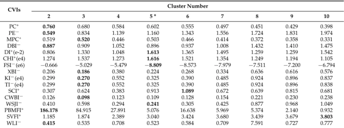
Table 7.Variations of the 16 CVIs with cluster numbers ranging from 2 to 10 for the FLC1 image.

CVIs Cluster Number

2 3 4 5 * 6 7 8 9 10 PC+ _{0.760 0.680 0.584 0.602 0.555 0.497 0.451 0.429 0.398} PE´ _{0.549 0.834 1.139 1.160 1.343 1.556 1.724 1.831 1.974} MPC+ _{0.519 0.520 0.446 0.503 0.466 0.414 0.372 0.358 0.331} DBI´ _{0.887 0.909 1.052 0.896 0.937 1.008 1.432 1.410 1.475} DI+_{(e-2) 0.806 1.330 1.048 1.613 1.365 1.495 1.259 1.259 1.542} CHI+_{(e4) 1.274 1.537 1.273 1.616 1.521 1.354 1.249 1.194 1.105} FSI´_{(e6) ´0.666 ´5.029 ´5.479 ´8.809 ´8.573 ´7.979 ´7.511 ´7.200 ´6.794} XBI´ _{0.206 0.186 0.380 0.224 0.268 0.334 0.636 0.616 0.576} KI´_{(e4) 0.299 0.270 0.552 0.325 0.390 0.485 0.924 0.896 0.837} TI´_{(e4) 0.299 0.270 0.552 0.325 0.390 0.485 0.924 0.896 0.838} SCI+ _{0.307 0.624 0.383 0.913 1.089 0.672 0.639 0.815 0.681} CWBI´ _{0.126 0.098 0.123 0.109 0.128 0.154 0.221 0.230 0.238} WSJI´ _{0.410 0.598 0.294 0.241 0.305 0.425 0.877 0.968 1.049} PBMFI+ _{186.178 84.915 27.891 5.076 16.638 5.969 5.374 2.140 0.932} SVFI+ _{1.185 1.874 2.389 3.040 3.424 3.680 3.439 3.679 3.803} WLI´ _{0.415 0.535 0.708 0.523 0.584 0.709 7.591 0.727 0.777}

Table 8.Variations of the 16 CVIs with cluster numbers ranging from 2 to 10 for the Hyperion image.

CVIs Cluster Number

2 3 4 * 5 6 7 8 9 10 PC+ _{0.867 0.759 0.682 0.658 0.596 0.568 0.530 0.494 0.476} PE´ _{0.337 0.626 0.869 0.973 1.176 1.293 1.435 1.577 1.666} MPC+ _{0.735 0.638 0.576 0.573 0.515 0.496 0.463 0.430 0.417} DBI´ _{0.472 0.651 0.732 0.726 0.853 0.856 0.946 1.060 1.032} DI+_{(e-2) 2.169 2.979 2.837 2.900 3.489 3.332 3.518 2.971 3.916} CHI+_{(e4) 4.690 5.329 5.328 5.779 5.485 5.383 5.158 4.925 4.846} FSI´_{(e11) ´4.610 ´6.600 ´6.902 ´7.003 ´6.808 ´6.619 ´6.414 ´6.209 ´6.039} XBI´ _{0.061 0.139 0.157 0.149 0.217 0.193 0.228 0.275 0.239} KI´_{(e3) 1.131 2.552 2.888 2.750 3.995 3.560 4.201 5.064 4.400} TI´_{(e3) 1.131 2.555 2.892 2.755 4.004 3.569 4.213 5.080 4.416} SCI+ _{2.241 3.109 3.161 4.201 4.012 4.586 4.574 4.469 4.605} CWBI´_{(e-3) 0.440 0.485 0.597 0.651 0.900 0.929 1.118 1.347 1.333} WSJI´ _{0.244 0.681 0.207 0.244 0.446 0.491 0.706 1.019 1.020} PBMFI+_{(e6) 4.131 6.247 1.732 0.319 0.528 0.325 0.184 0.009 0.005} SVFI+ _{2.204 2.459 2.867 3.124 3.307 3.536 3.697 3.764 3.885} WLI´ _{1.222 0.185 0.241 0.231 0.242 0.244 0.254 0.281 0.307}

Note:*denotes the actual cluster number of the image.

Table 9.Variations of the 16 CVIs with cluster numbers ranging from 2 to 10 for the HYDICE image.

CVIs Cluster Number

2 3 4 * 5 6 7 8 9 10 PC+ _{0.752 0.729 0.669 0.621 0.587 0.554 0.541 0.511 0.502} PE´ _{0.573 0.717 0.922 1.106 1.246 1.382 1.471 1.598 1.656} MPC+ _{0.504 0.594 0.558 0.526 0.505 0.479 0.475 0.450 0.447} DBI´ _{0.888 0.669 0.747 0.824 0.828 0.899 0.827 0.888 0.888} DI+_{(e-2) 1.194 1.070 1.165 1.236 1.081 1.190 1.897 1.098 1.089} CHI+_{(e4) 1.057 1.494 1.473 1.618 1.606 1.508 1.634 1.587 1.594} FSI´_{(e12) 0.004 ´1.258 ´1.511 ´1.592 ´1.627 ´1.603 ´1.608 ´1.579 ´1.567} XBI´ _{0.196 0.105 0.149 0.168 0.231 0.258 0.223 0.315 0.260} KI´_{(e3) 2.025 1.084 1.545 1.733 2.393 2.671 2.306 3.258 2.694} TI´_{(e3) 2.026 1.085 1.547 1.737 2.398 2.678 2.313 3.268 2.704} SCI+ _{0.391 1.878 1.906 1.997 2.151 1.733 1.911 1.691 1.901} CWBI´_{(e-4) 2.538 1.761 2.017 2.395 3.082 3.508 3.585 4.598 4.398} WSJI´ _{0.422 1.082 0.229 0.299 0.482 0.621 0.671 1.111 1.034} PBMFI+_{(e6) 27.978 28.242 7.311 1.490 2.274 1.228 0.250 0.655 0.118} SVFI+ _{1.560 2.490 2.928 3.298 3.566 3.689 4.202 4.352 4.349} WLI´ _{0.390 0.263 0.288 0.323 0.388 0.406 0.475 0.474 0.387}

Note:*denotes the actual cluster number of the image.

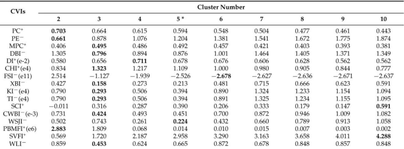
Table 10.Variations of the 16 CVIs with cluster numbers ranging from 2 to 10 for the ROSIS image.

CVIs Cluster Number

2 3 4 5 * 6 7 8 9 10 PC+ _{0.703 0.664 0.615 0.594 0.548 0.504 0.477 0.461 0.443} PE´ _{0.661 0.878 1.076 1.204 1.381 1.541 1.672 1.775 1.874} MPC+ _{0.406 0.495 0.486 0.492 0.457 0.421 0.403 0.393 0.381} DBI´ _{1.305 0.796 0.894 0.876 1.001 1.464 1.405 1.371 1.349} DI+_{(e-2) 0.580 0.656 0.711 0.678 0.676 0.606 0.628 0.562 0.562} CHI+_{(e4) 0.834 1.323 1.217 1.109 1.000 0.980 0.905 0.844 0.777} FSI´_{(e11) 2.514 ´1.127 ´1.939 ´2.526 ´2.678 ´2.627 ´2.636 ´2.671 ´2.637} XBI´ _{0.427 0.158 0.273 0.213 0.481 0.715 0.666 0.623 0.591} KI´_{(e4) 0.790 0.293 0.506 0.394 0.890 1.324 1.233 1.154 1.094} TI´_{(e4) 0.790 0.293 0.506 0.394 0.891 1.325 1.234 1.155 1.095} SCI+ _{´0.011 0.316 0.287 0.390 0.206 0.333 0.179 0.147 0.591} CWBI´_{(e-3) 0.731 0.424 0.493 0.451 0.700 0.872 0.946 1.009 1.082} WSJI´ _{0.502 0.743 0.261 0.224 0.432 0.660 0.789 0.913 1.058} PBMFI+_{(e6) 2.883 1.809 0.068 0.014 0.010 0.015 0.007 0.003 0.002} SVFI+ _{0.569 1.720 2.187 2.958 3.290 3.163 3.658 4.011 4.288} WLI´ _{0.859 0.453 0.624 0.665 0.872 0.678 0.848 0.857 0.848}

Remote Sens.2016,8, 295 16 of 22

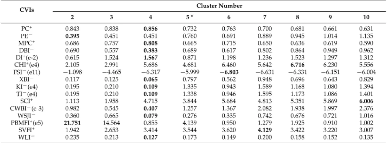
Table 11.Variations of the 16 CVIs with cluster numbers ranging from 2 to 10 for the AVIRIS image.

CVIs Cluster Number

2 3 4 5 * 6 7 8 9 10 PC+ _{0.843 0.838 0.856 0.732 0.763 0.700 0.681 0.661 0.631} PE´ _{0.395 0.451 0.451 0.760 0.691 0.889 0.945 1.014 1.135} MPC+ _{0.686 0.757 0.808 0.665 0.715 0.650 0.636 0.619 0.590} DBI´ _{0.690 0.557 0.383 0.689 0.617 0.802 0.864 0.949 0.962} DI+_{(e-2) 0.615 1.524 1.567 0.871 1.198 1.236 1.523 1.297 1.312} CHI+_{(e4) 2.105 2.991 5.686 4.681 6.460 5.642 6.716 6.230 5.556} FSI´_{(e11) ´1.098 ´4.465 ´6.317 ´5.999 ´6.803 ´6.631 ´6.331 ´6.151 ´6.004} XBI´ _{0.117 0.125 0.065 0.797 0.562 0.948 0.696 0.643 0.829} KI´_{(e4) 0.195 0.210 0.109 1.335 0.943 1.589 1.168 1.080 1.394} TI´_{(e4) 0.195 0.210 0.109 1.338 0.946 1.595 1.173 1.086 1.401} SCI+ _{1.113 1.958 4.715 3.844 5.684 4.813 5.351 5.869 6.006} CWBI´_{(e-3) 0.982 0.545 0.407 1.257 1.367 2.082 1.938 1.997 2.376} WSJI´ _{0.360 0.665 0.079 0.276 0.335 0.742 0.676 0.721 1.016} PBMFI+_{(e5) 21.751 14.564 0.855 4.139 0.950 1.279 1.925 0.910 1.002} SVFI+ _{1.942 2.653 3.414 3.544 3.620 4.129 3.422 3.220 3.007} WLI´ _{0.235 0.213 0.127 0.173 0.149 0.200 0.158 0.152 0.135}

Note:*denotes the actual cluster number of the image.

Figure3a–d shows the clustering results of the simple QuickBird image with the cluster number K“2, 3, 4, 5. The three ground truth classes (road, paddy field, and farmland) of the image were well identified with cluster numberK“3 (Figure3b). As listed in Table3, the majority of CVIs correctly indicated the actual cluster number of this simple image (except CHI, FSI, SCI, and SVFI).

Figure3e-h illustrates the clustering results of the Landsat TM image with the cluster number K“2, 3, 4, 5. Among them, the clustering withK“4 succeeded in separating the four ground truth classes of the image (forest, farmland, water, and town) (Figure3g). The clustering withK“2 was obviously incorrect since three ground truth classes,i.e., forest, farmland, and town were merged into one class (Figure3e). Unfortunately, as shown in Table4most indices (DBI, PC, PE, MPC, XBI, KI, TI, PBMFI, and WLI) underestimated the real situation, which preferred two as the cluster number of the image; whereas a clear overestimation was given by DI and SVFI; only five CVIs including CHI, FSI, SCI, CWBI, and WSJI provided the actual cluster number of the image.

Figure3i–l portrays the clustering results of the Landsat ETM+ image with the cluster number K “2, 3, 4, 5, respectively. The four ground truth classes of the image (marsh, forest, water, and farmland) were well separated with cluster numberK“4 (Figure3k). However, similar to the Landsat TM experiment, most indices (PE, MPC, XBI, KI, TI, CWBI, PBMFI, and WLI) recommended two clusters as the optimal partitioning of the image (Table5). CHI and WSJI were the only two indices that correctly indicated the cluster number of the image.

Figure3m–p presents the clustering results of the GaoFen-1 image with the cluster number K“2, 4, 5, 6. The five ground truth classes of the image, namely water1 (light colored), water2 (dark colored), grass, soil, and sand, were well distinguished with cluster numberK“5 (Figure3o). This was correctly indicated by most CVIs including DBI, CHI, MPC, FSI, XBI, KI, TI, SCI, WSJI, and WLI (Table6). For the rest of the CVIs that erroneously indicated the cluster number, most of them (DI, PC, PE, and PBMFI) suggested two.

Figure3q–t demonstrates the clustering results of the FLC1 image with the cluster number K“2, 3, 5, 6. The five ground truth classes of the image (soybeans, oats, corn, wheat, and red clover) were fairly well identified with cluster numberK “5 (Figure3s). For the cases of clustering with K“2 andK“3, obvious misclassifications were observed, with some separated classes being merged into one class (Figure3q,r). As shown in Table7, there were four CVIs (DI, CHI, FSI, and WSJI) that provided the actual cluster number (K “5) for the image. But five CVIs (DBI, PC, PE, PBMFI, and WLI) and five others (MPC, XBI, KI, TI, and CWBI) erroneously supported the clustering with cluster numberK“2 andK“3, respectively.

Figure4a–d depicts the clustering results of Hyperion data with the cluster numberK“2, 3, 4, 5. The four ground truth classes (woodland, island interior, water, and floodplain grasses) were well classified with cluster numberK“4 (Figure4c). Clustering results with other cluster numbers were

obviously not satisfactory. For example, in the case of clustering withK“2, three (without water) of the four classes were wrongly merged into one class (Figure4a). This was chosen by half the total CVIs, namely DBI, PC, PE, MPC, XBI, KI, TI, and CWBI (Table8). In fact, all of the CVIs, except WSJI, failed to detect the actual cluster number of the image.

Figure4e–h provides the clustering results of HYDICE data with the cluster numberK“3, 4, 5, 6, of which the clustering withK“4 properly separated the four ground truth classes (roads, trees, trail, and grass) (Figure4f). In the case of clustering withK“3, there were clear errors due to the incorrect merging of trees and roads (Figure4e). However, it was still suggested by half of the CVIs, including DBI, MPC, XBI, KI, CWBI, TI, PBMFI, and WLI (Table9). Similar to the experiment on Hyperion, WSJI was the only index returning the correct information about cluster number.

Figure4i–l lists the clustering results of ROSIS data with the cluster number K “ 3, 4, 5, 6. Among them, the clustering withK“5 successfully classified the five ground truth classes (meadows, trees, asphalt, bricks, and shadows) (Figure4k). For the case ofK“3, trees and shadows were not distinguished (Figure4i). However, this incorrect suggestion was also made by as many as half of the CVIs, including DBI, CHI, MPC, XBI, KI, TI, CWBI, and WLI (Table10). Once again, only WSJI correctly indicated the actual cluster number of the image.

Figure4m–p shows the clustering results of AVIRIS data with the cluster numberK“3, 4, 5, 6, in which the five ground truth classes (vineyard untrained, celery, fallow smooth, fallow plow, and stubble) were well classified withK“5 (Figure4o). However, no CVI was able to indicate the actual cluster number of the image (Table11). Instead, most of them (DBI, DI, PC, MPC, XBI, KI, TI, CWBI, WSJI, and WLI) preferred four clusters for the image, which merged the classes of fallow smooth and fallow plow (Figure4n).

Figure5illustrates the percentage of successes (correct guesses) achieved by the 16 CVIs. Table12 summarizes the cluster validity results of the 16 CVIs by FCM on nine types of remote sensing image datasets, in which the actual cluster number of each image is listed in column K# while those indicated by CVIs are shown in other columns. From the table it can be seen that WSJI was the only index that correctly recognized the actual cluster numbers of all of the datasets (including multispectral and hyperspectral data), except for the AVIRIS image. Thus WSJI, was the most effective and stable index of all. CHI and FSI succeeded in multispectral datasets but failed in hyperspectral datasets. The DBI, DI, MPC, SCI, XBI, KI, TI, CWBI, and WLI indices were only effective for two multispectral images. CVIs including PC, PE, and PBMFI failed, generally, except for the simple QuickBird experiment. SVFI failed for all images.

Remote Sens. 2016, 8, 295 18 of 23

(meadows, trees, asphalt, bricks, and shadows) (Figure 4k). For the case of

K

=

3

, trees and shadows were not distinguished (Figure 4i). However, this incorrect suggestion was also made by as many as half of the CVIs, including DBI, CHI, MPC, XBI, KI, TI, CWBI, and WLI (Table 10). Once again, only WSJI correctly indicated the actual cluster number of the image.

Figure 4m–p shows the clustering results of AVIRIS data with the cluster number

6

,

5

,

4

,

3

=

K

, in which the five ground truth classes (vineyard untrained, celery, fallow smooth, fallow plow, and stubble) were well classified with

K

=

5

(Figure 4o). However, no CVI was able to indicate the actual cluster number of the image (Table 11). Instead, most of them (DBI, DI, PC, MPC, XBI, KI, TI, CWBI, WSJI, and WLI) preferred four clusters for the image, which merged the classes of fallow smooth and fallow plow (Figure 4n).

Figure 5 illustrates the percentage of successes (correct guesses) achieved by the 16 CVIs. Table 12 summarizes the cluster validity results of the 16 CVIs by FCM on nine types of remote sensing image datasets, in which the actual cluster number of each image is listed in column K# while those indicated by CVIs are shown in other columns. From the table it can be seen that WSJI was the only index that correctly recognized the actual cluster numbers of all of the datasets (including multispectral and hyperspectral data), except for the AVIRIS image. Thus WSJI, was the most effective and stable index of all. CHI and FSI succeeded in multispectral datasets but failed in hyperspectral datasets. The DBI, DI, MPC, SCI, XBI, KI, TI, CWBI, and WLI indices were only effective for two multispectral images. CVIs including PC, PE, and PBMFI failed, generally, except for the simple QuickBird experiment. SVFI failed for all images.

Figure 5. The overall performance of CVIs by applying FCM algorithm to cluster nine types of remote sensing datasets.

Table 12. The optimal cluster numbers indicated by the CVIs by FCM for each remote sensing image.

Images K# PC PE MPC DBI DI CHI FSI SCI

Multispectral image QuickBird 3 3 * 3 * 3 * 3 * 3 * 8 8 8 Landsat TM 4 2 2 2 2 7 4 * 4 * 4 * Landsat ETM+ 4 3 2 2 2 5 4 * 3 7 GaoFen-1 5 2 2 5 * 5 * 2 5 * 5 * 5 * FLC1 5 2 2 3 2 5 * 5 * 5 * 6 Hyperspectral image Hyperion 4 2 2 2 2 10 5 6 10 HYDICE