NBER WORKING PAPER SERIES
VENTURE CAPITAL CONTRACTING AND SYNDICATION: AN EXPERIMENT IN COMPUTATIONAL CORPORATE FINANCE
Zsuzsanna Fluck Kedran Garrison Stewart C. Myers Working Paper11624
http://www.nber.org/papers/w11624
NATIONAL BUREAU OF ECONOMIC RESEARCH 1050 Massachusetts Avenue
Cambridge, MA 02138 September 2005
We are grateful for helpful comments from Ulf Axelson, Amar Bhide, Francesca Cornelli, Paul Gompers, Steve Kaplan, Josh Lerner, Tom Noe, David Scharfstein, Per Str¡§omberg, Michael Weisbach and participants at presentations at LSE, MIT, Michigan State University, the University of Minnesota, the Conference on Venture Capital and Private Equity (Stockholm), the Financial Intermediation Research Society Conference (Capri) and the American Finance Association meetings (Philadelphia). The views expressed herein are those of the author(s) and do not necessarily reflect the views of the National Bureau of Economic Research.
©2005 by Zsuzsanna Fluck, Kedran Garrison and Stewart C. Myers. All rights reserved. Short sections of text, not to exceed two paragraphs, may be quoted without explicit permission provided that full credit, including © notice, is given to the source.
Venture Capital Contracting and Syndication: An Experiment in Computational Corporate Finance
Zsuzsanna Fluck, Kedran Garrison and Stewart C. Myers NBER Working Paper No. 11624
September 2005 JEL No. G24, G32
ABSTRACT
This paper develops a model to study how entrepreneurs and venture-capital investors deal with moral hazard, effort provision, asymmetric information and hold-up problems. We explore several financing scenarios, including first-best, monopolistic, syndicated and fully competitive financing. We solve numerically for the entrepreneur's effort, the terms of financing, the venture capitalist's investment decision and NPV. We find significant value losses due to holdup problems and under-provision of effort that can outweigh the benefits of staged financing and investment. We show that a commitment to later-stage syndicate financing increases effort and NPV and preserves the option value of staged investment. This commitment benefits initial venture capital investors as well as the entrepreneur.
Zsuzsanna Fluck
Michigan State University Department of Finance
Graduate School of Management 315 Eppley Center East Lansing, MI 48824-1122 fluck@bus.msu.edu Kedran Garrison MIT - EFA 77 Massachusetts Avenue Cambridge, MA 02139-4307 garrisk@mit.edu Stewart C. Myers
Sloan School of Management MIT, Room E52-451
50 Memorial Drive
Cambridge, MA 02142-1347 and NBER
1
Introduction
This paper develops a model to study how entrepreneurs and venture-capital investors deal with effort provision, moral hazard, asymmetric information and hold-up problems when contracts are incomplete and investment proceeds in stages. How much value is lost in the entrepreneur-venture capital relationship relative to first-best value? How does the value lost depend on risk and the time-pattern of required investment? What determines whether a positive-NPV project can in fact befinanced? What are the advantages and disadvantages of staged financing? Are there significant efficiency gains from syndication of later-stage
financing?
We argue that these and related questions should not be analyzed one by one, but jointly in a common setting. Some features of venture-capital contracting may not solve a particular problem, but instead trade off one problem against another. For example, a study that focused just on the option-like advantages of staged investment could easily miss the costs of staging, particularly the negative feedback to effort if venture-capital investors can hold up the entrepreneur by dictating financing terms in later stages. (We find many cases where hold-up costs outweigh the advantages of staged financing and full upfront financing actually increases value.)
A joint analysis of the problems inherent in the entrepreneur-venture capital relationship does not lead to closed-form solutions or simple theorems. Therefore we embark on an experiment in computational corporate finance, which is the formal study of financing and investment problems that do not have closed-form solutions.1 We believe the time is ripe for a computational model of venture capital. Venture-capital institutions, contracts and procedures were well documented more than a decade ago. It was clear then that the agency and information problems encountered in ordinary financing decisions are especially acute in venture capital. The successes of venture capital have stimulated theoretical work on how these problems are mitigated. But most theoretical papers have focused on only one problem or tradeoff and run the risk of missing the bigger picture.
Of course the breadth and richness of a computational model do not come free, and numerical results are never absolutely conclusive. One can never rule out the possibility that results would have been different with different inputs or modeling choices. But our model, though simplified, follows actual practice in venture capital. We have verified our main results over a wide range of inputs. We believe our results help to clarify why venture-capital investment works when it works and why it sometimes fails.
The structure of venture-capitalfinancing is known from many sources, including Sahlman (1990), Lerner (1994), Fenn, Liang and Prowse (1995), Gompers (1995), Gompers and Lerner (1996, 2002), Hellman and Puri (2000, 2002) and Kaplan and Str¨omberg (2003). We will preview our model and results after a brief review of the features of venture-capital con-tracting that are most important to our paper. The review includes comments on related 1Computational models are frequently used to understand the value of real and financial options, but
their use on the financing side of corporate balance sheets is an infant industry. The short list of com-putational papers on financing includes Mello and Parsons (1992), Leland (1994, 1998), Boyd and Smith (1994), Parrino and Weisbach (1999), Robe (1999, 2001), Parrino, Poteshman and Weisbach (2002) and Ju, Parrino, Poteshman and Weisbach (2004). These papers explore the tradeofftheory of capital structure and the risk-shifting incentives created by debtfinancing.
theoretical work.
1.1
Venture capital contracting
Venture capital brings together one or more entrepreneurs, who contribute ideas, plans, hu-man capital and effort, and private investors, who contribute experience, expertise, contacts and most of the money. For simplicity, we will refer to one entrepreneur and to one initial venture-capital investor. Their joint participation creates a two-way incentive problem. The investor has to share financial payoffs with the entrepreneur in order to secure her commit-ment and effort. Thus the investor may not be willing to participate even if the startup has positive overall NPV. Second, the entrepreneur will underinvest in effort if she has to share her marginal value added with the investor.2
1.1.1 Sweat equity
The entrepreneur invests even when she puts up none of the financing. She contributes her effort and absorbs part of the firm’s business risk. The difference between her salary and her outside compensation is an opportunity cost. Specialization of her human capital to the new firm also creates an opportunity cost if the firm fails.3
The entrepreneur receives shares in exchange for these investments. These shares may not vest immediately, and they are illiquid unless and until the firm is sold or goes public.4 The venture capitalist frequently requires the entrepreneur to sign a contract that precludes work for a competitor. The entrepreneur therefore has a strong incentive to stick with the firm and make it successful. In our model, the entrepreneur contributes no financial investment and is willing to continue so long as the present value of her shares exceeds her costs of effort. 1.1.2 Staged investment and financing
A startup is a compound call option. Financing and investment are made in stages. The stages match up with business milestones, such as a demonstration of technology or a suc-cessful product introduction.
We assume that the entrepreneur and venture capitalist cannot write a complete contract to specify the terms of futurefinancing. The terms are determined by bargaining asfinancing is raised stage by stage. If additional investors join in later stages, the bargain has to be acceptable to them as well as the entrepreneur and initial venture capitalist.
The option value added by staging is obvious, but staging may also serve other purposes. In Bergemann and Hege (1998) and N¨oldeke and Schmidt (1998), staging allows the venture capitalist to learn the startup’s value and thereby induce the entrepreneur’s effort. In Neher
2This is an extreme version of Myers’s (1977) underinvestment problem.
3This opportunity cost could perhaps be reduced if new ventures are developed as divisions of larger firms. See Gromb and Scharfstein (2003) and Gompers, Lerner and Scharfstein (2003).
4Employees typically receive options that vest gradually as employment continues and the startup
sur-vives. But our entrepreneur is a founder, not an employee hired later. Founders typically receive shares, not options. The entrepreneur’s shares are fully vested, but additional shares may be granted later. See Kaplan and Str¨omberg (2003).
(1996) and Landier (2002), the venture capitalist’s ability to deny financing at each stage forces the entrepreneur to exert higher effort and prevents her from diverting cashflows.
Venture capital investors usually buy convertible preferred shares. If the firm is shut down, the investors have a senior claim on any remaining assets. The shares convert to common stock if the firm is sold or taken public.5 Ordinary debt financing is rarely used, although we will consider whether debt could serve as an alternative source of financing. 1.1.3 Control
The venture capitalist does not have complete control of the newfirm. For example, Kaplan and Str¨omberg (2003, Table 2)find that venture-capital investors rarely control a majority of the board of directors. But Kaplan and Str¨omberg also find that venture capitalists’ control increases when thefirm’s progress is unsatisfactory.
Staged financing can give incumbent venture capitalists effective control over access to
financing. Their refusal to participate in the second or later rounds offinancing would send a strong negative signal to other potential investors and probably deter them from investing.6 In practice, the incumbents’ decision not to participate is usually a decision to shut down the firm.
Giving venture capitalists effective veto power over later-stage investment is in some respects efficient. The decision to shut down or continue cannot be left to the entrepreneur, who is usually happy to continue investing someone else’s money as long as there is any chance of success. The venture capitalist is better equipped to decide whether to exercise each stage of the compound call option.
Thus stagedfinancing has a double benefit, at least for the venture capitalist. It can block the entrepreneur’s incentive to continue and it allows the venture capitalist to exploit the startup’s real-option value. But it is also costly if the venture capitalist can use the threat of shutdown to hold up the entrepreneur and dilute her stake. Anticipated dilution feeds back into the entrepreneur’s incentives and effort and reduces overall value. This is the holdup problem of staged financing. For a wide range of parameter values we find that the holdup problem is so severe that the venture capitalist is better offabandoning stagedfinancing and providing all financing upfront. When later financing stages are syndicated on competitive terms, however, stagedfinancing is always more efficient than full upfront financing. We will also show that the holdup problem cannot be solved simply by substituting debt for equity
financing. When contracts are incomplete, stage by stage bargaining enables the incumbent venture capitalist to extract surplus regardless of the form of financing.
Most prior theory assumes that venture-capital investors retain residual rights of control. The venture capitalist’s rights to decide on investment (Aghion and Bolton (1992)) and to replace the entrepreneur (Fluck (1998), Hellman (1998), Myers (2000), Fluck (2001)) play an important role in enforcingfinancial contracts between investors and entrepreneurs. The 5The use of convertible securities in venture capital is analyzed in Green (1984), Berglof (1994), Kalay
and Zender (1997), Repullo and Suarez (1998), Cornelli and Yosha (2003), Schmidt (2003) and Winton and Yerramilli (2003).
6The role of the monopolistfinancier was investigated in Rajan (1992), Petersen and Rajan (1994) and
entrepreneur’s option to reacquire control and realize value in an initial public offering is a key incentive in Black and Gilson (1998), Myers (2000) and Aghion, Bolton and Tirole (2001).
1.1.4 Syndication of later-stage financing
Later-stage financing usually comes from a syndicate of incumbent and new venture-capital investors. We show how a commitment to syndicate can alleviate the holdup problem by assuring the entrepreneur more favorable terms in later rounds offinancing. This encourages effort in all periods, which increases overall value.
Syndication of venture capital investments has been explained in several other ways. It is one way to gather additional information about a startup’s value — see, for example, Gompers and Lerner (2002, Ch. 9) and Sah and Stiglitz (1986). Wilson (1968) attributes syndication to venture capitalists’ risk aversion. Syndication may also reflect tacit collusion: early investors syndicate later rounds of financing, and the syndication partners return the favor when they develop promising startups (Pichler and Wilhelm (2001)). In Cassamatta and Haritchabalet (2004), venture capitalists acquire different skills and experience and syndication pools their expertise. We offer a different rationale: syndication can protect the entrepreneur from ex post holdup by investors and thereby encourage effort.
1.1.5 Exit
Entrepreneurs can rely on venture capitalists to cash out of successful startups. Venture capital generally comes from limited-life partnerships, and the partners are not paid until the startups are sold or taken public. Myers (2000) shows that venture capitalists would cash out voluntarily in order to avoid the adverse incentives of long-term private ownership. Chelma, Habib and Lyngquist (2002) consider how the various provisions of venture-capital contracts are designed to mitigate multiple agency and information problems. Their paper focuses on exit provisions and does not consider syndication.
1.2
Preview of the model and results
We aim to capture the most important features of venture capital. For simplicity we assume two stages of financing and investment at dates 0 and 1. If successful, the firm is sold or taken public at date 2, and the entrepreneur and the investors cash out. The entrepreneur and the investors are risk-neutral NPV maximizers, although the entrepreneur’s NPV is net of the costs of her effort.
We value the startup as a real option. The underlying asset is the potential market value of the firm, which we assume is lognormally distributed. But full realization of potential value requires maximum effort from the entrepreneur at dates 0 and 1. The entrepreneur’s effort is costly, so her optimal effort is less than the maximum and depends on her expected share of the value of thefirm at date 2. The venture capitalist and the entrepreneur negotiate ownership percentages at date 0, but these percentages change at date 1 when additional
We assume that the firm cannot start or continue without the entrepreneur. If financing cannot be arranged on terms that satisfy her participation constraints, no investment is made and the firm shuts down. The venture capitalist’s date-0 and date-1 participation constraints must also be met, since he will not invest if his NPV is negative.
The efficiency of venture-capital investment hinges on the nature and terms of financing. We compare six cases.
1. First-best. If the entrepreneur could finance the startup out of her own pocket, she would maximize overall value, net of the required financial investments and her costs of effort. First-best is our main benchmark for testing the efficiency of other cases. 2. Fully competitive. In this case, financing is available on competitive terms (NPV = 0)
at both date 0 and date 1, which gives the highest possible value when the entrepreneur must raise capital from outside investors. We include this case as an alternative bench-mark to first-best.
3. Monopoly, staged investment. Here the initial venture capitalist can dictate the terms offinancing at dates 0 and 1 and can hold up the entrepreneur at date 1.7 The venture capitalist does not squeeze the last dollar from the entrepreneur’s stake, however. He squeezes just enough in each period to maximize the present value of his shares. 4. Monopoly, no staging. In this case, the venture capitalist commits all necessary funds
at date 0 and lets the entrepreneur decide whether to continue at date 1. This means inefficient investment decisions at date 1, because the entrepreneur is usually better off continuing, even when the odds of success are low and overall NPV is negative. But effort increases at both date 0 and date 1, because the venture capitalist can no longer control the terms of later-stage financing. This case helps clarify the tradeoff between the real-option value of staged investment and the under-provision of effort because of the holdup problem.
5. Syndication. In this case a syndicate of additional investors joins the original venture capitalist at date 1. We assume that the syndicate financing comes on more com-petitive terms than in the monopoly case, for simplicity we will focus on the fully competitive case (NPV = 0). Syndication mitigates the holdup problem, increasing the entrepreneur’s effort and overall NPV.
6. Debt. Venture capitalists rarely finance startups with ordinary debt, but we neverthe-less consider debt financing briefly as an alternative. Debt financing effectively gives the entrepreneur a call option on the startup’s final value at date 2.
We assume that the initial venture capitalist and the entrepreneur are equally informed about potential value, although potential value is not verifiable and contractible. But fi -nancing terms in the syndication case depend on the information available to new investors. We start by assuming complete information, but also consider asymmetric information and explore whether the terms of the incumbent venture capitalist’s participation in date-1 fi -nancing could reveal the incumbent’s inside information.
7This would be the case if the venture capitalist decided that certain non-verifiable performance milestones
We solve the model for each financing case over a wide range of input parameters, in-cluding the potential value of thefirm, the variance of this value, the amount and timing of required investment and the marginal costs and payoffs of effort. We report a representative subset of results in Table 1 and Figures 3 through 10. Results are especially sensitive to the marginal costs and payoffs of effort, so we vary these parameters over very wide ranges. Our main results include the following:
1. Wefind economically significant value losses, relative tofirst best, even when the dollar-equivalent cost of effort is a small fraction of requiredfinancial investment. Thus many startups with positive NPVs cannot be financed. Value losses decline as the marginal benefit of effort increases or the marginal cost declines.
2. Value losses are especially high in the monopoly case with staged investment, where the incumbent venture capitalist can dictate the terms of financing at date 1. For a wide range of parameter values, both the venture capitalist and entrepreneur are better off in the no-staging case with full upfront financing. That is, the costs of the no-staging case (inefficient investment at date 1) can be less than the value loss due to under-provision of effort in the monopoly, staged financing case.
3. Syndicate financing at date 1 increases effort and the date-0 NPVs of both the en-trepreneur and the initial venture capitalist. The venture capitalist is better off than in the monopoly case, despite taking a smaller share of the venture. Moreover, staged
financing with syndication always produces higher overall values than the no-staging case. The combination of staged financing and later-stage syndication dominates the alternative of giving the entrepreneur all the money upfront.
4. Syndicatefinancing is most effective when new investors are fully informed. The incum-bent venture capitalist may be able to reveal his information through his participation in date-1 financing. However, the fixed-fraction participation rule derived by Admati and Pfleiderer (1994) does not achieve truthful information revelation in our model, because the terms of financing effect the entrepreneur’s effort. Thefixed-fraction rule would lead the venture capitalist to over-report the startup’s value: the higher the price paid by new investors, the more the entrepreneur’s existing shares are worth, and the harder she works. The incumbent venture capitalist captures part of the gain from her extra effort. A modifiedfixed-fraction rule works in some cases, however. With the modified rule, the incumbent’s fractional participation increases as the reported value increases.
5. We expected venture-capital contracting to be more efficient for high-variance invest-ments, but that is not generally true. Increasing the variance of potential value some-times increases value losses, relative to first best, and sometimes reduces them, de-pending on effort parameters and the financing case assumed.
6. Debt financing does not solve the holdup problem, because the venture capitalist can still squeeze the entrepreneur by demanding a high interest rate on debt issued at date 1. Debt financing is more efficient in some cases but not generally. Debt can improve the entrepreneur’s incentives at laterfinancing stages, but many startups that can be
debtfinancing does add value in some cases, but not generally. In most cases, syndicate
financing with equity rather than debt increases both overall NPV and the NPV to the original venture capitalist.
We recognize that we have left out several aspects of venture capital that could influence our results. First, we ignore risk aversion. The venture capitalist and entrepreneur are assumed risk-neutral. This is reasonable for venture capitalists, who have access to financial markets.8 It is less reasonable for entrepreneurs, who can’t hedge or diversify payoffs without damaging incentives.9
Second, we do not explicitly model the costs and value added of the venture capitalist’s effort. We are treating his effort as a cost sunk at startup andfixed afterwards. In effect, we assume that if the venture capitalist decides to invest, he will exert appropriate effort, and that the cost of this effort is rolled into the required investment.
Third, we assume that final payoffs to the entrepreneur and venture-capital investors depend only on the number of shares bargained for at dates 0 and 1. We do not explic-itly model the more complex, contingent contracts observed in some cases by Kaplan and Str¨omberg (2003),10 and we do not attempt to derive the optimalfinancial contracts for our model setup. However, our results in Section 4 suggest that the use of contingent share awards may facilitate truthful revelation of information by the initial venture capitalist to members of a later-stage financing syndicate.
Finally, we do not model the search and screening processes that bring the entrepreneur and venture capitalist together in the first place. The costs and effectiveness of these pro-cesses could affect the terms offinancing.11 For example, if an entrepreneur’s search for alter-nativefinancing would be cheap and quick, the initial venture capitalist’s bargaining power is reduced. Giving the entrepreneur the option to search for another initial investor would not change the structure of our model, however. It would simply tighten the entrepreneur’s par-ticipation constraint at date 0 and thereby reduce the intial venture capitalist’s bargaining power.
The rest of this paper is organized as follows. Section 2 sets up our model and solves the first-best case. Section 3 covers monopoly financing with and without staging. Section 4 covers the syndication and fully competitive cases. Numerical results are summarized and interpreted in Section 5. Section 6 briefly considers debt financing. Section 7 sums up our conclusions and notes questions remaining open for further research.
8Of course, the venture capitalist will seek an expected rate of return high enough to cover the market
rate of risk in the startup. The payoffs in our model can be interpreted as certainty equivalents.
9Perhaps the entrepreneur’s risk aversion is cancelled out by optimism. See Landier and Thesmar (2003). 10Kaplan and Str¨omberg (2003, Table 3)find contingent contracts in 73% of thefinancing rounds in their
sample. The most common contingent contract depends on the founding entrepreneur staying with thefirm, for example a contract requiring the entrepreneur’s shares to vest. Vesting is implicit in our model, because the entrepreneur gets nothing if thefirm is shut down at date 1. Contingent contracts are also triggered by sale of securities, as in IPOs, or by default on a dividend or redemption payment. But solving the incentive and moral hazard problems in our model would require contracts contingent on effort or interim performance, which are non-verifiable in our model. Such contracts are rare in Kaplan and Str¨omberg’s sample.
11Inderst and Muller (2003) present a model of costly search and screening, with bargaining and endogenous
effort by both the entrepreneur and the venture capitalist. Their model does not consider staged investment andfinancing.
2
Model Setup and the First-Best Case
The entrepreneur possesses a startup investment opportunity that requires investments I0 and I1 at dates 0 and 1. If both investments are made, the startup continues to date 2 and the final value of the firm is realized.
If the investment at date 1 is not made, or if the entrepreneur refuses to participate, the startup is shut down and liquidated. We assume for simplicity that liquidation value is zero. (It is typically small for high-tech startups.) This assumption simplifies our analysis of financing, because the venture capitalist’s preferred shares have value only if converted. Thus, we can treat these shares as if they were common in the first place.
The total payoff at date 2 is P, which is stochastic and depends on the entrepreneur’s effort at time 0 and time 1, x0 and x1, and onV2, the potential value of thefirm at date 2. Effort affects the payoff multiplicatively through the effort functions f0(x0) and f1(x1):
P =f0f1V2 (1)
Effort generates positive but decreasing returns, that is, f(0) = 0, f > 0 and f < 0. The entrepreneur bears the costs of her effort, g0(x0) and g1(x1). The effort cost function is strictly increasing and convex, that is,g(0) ≥0,g >0 and g >0.
The potential value V2 is the sole source of uncertainty. We define the expected value
E1(V2) at date 1 as V1 and expected value E0(V2) at date 0 as V0. The expected payoffs at dates 0 and 1, assuming that the firm will survive until date 2, are:
E1(P) =E1(f0f1V2) =f0f1E1(V2) =f0f1V1
E0(P) =E0(E1(P)) =f0E0(f1V1|V0)
(2) where E0(f1V1|V0) is an integral that accounts for the dependence of f1 on V1. We assume risk-neutrality and a risk-free interest rate of zero. We use lognormal probability distributions for V1 and V2, with standard deviationσ per period.
Define the effort function f and the effort cost function g as
ft = 1−e−θfxt
gt =eθgxt (3)
for t = 0,1. The effort function f asymptotes to 1, so we interpret V1 and V2 as maximum attainable values asx→ ∞. The degree of concavity and convexity of f and g depends on
θf and θg. The effort functions are plotted in Figure 1 for several values of θf and θg.
The timeline of the financing process is as follows:
−−−−−−−−−−−−−−−−−−−−−−−−−−−−−−−−−−−−−−−−−−−−−−−−−−−−−−−−−−→
t=0 t=1 t=2
V0 known V1 realized V2 realized
αC0 determined αC1 determined P =f0f1V2
I0,x∗0 invested if N P V0M ≥0 I1,x∗1 invested if N P V1M ≥0
and N P VC
First, the entrepreneur (M) goes to the initial venture capitalist (C) to raise startupfi nanc-ing. If he is willing to invest, then she and he negotiate the initial ownership shares αM
0 and αC
0. At date 1, V1 is observed and there is another round of bargaining over the terms of financing. If the initial venture capitalist also supplies all financing at date 1, then he can dictate the terms and his share becomes αC
1, with a corresponding adjustment in αM1 . If the initial venture capitalist brings in a syndicate of new investors at date 1, then the syndicate receives an ownership share of αS1, and αM1 and αC1 adjust accordingly. The terms of financing arefixed after date 1.
2.1
First-best
In the first-best case, the entrepreneur supplies all of the money,I0+I1, and owns the firm (αM
0 =αM1 = 1). The entrepreneur maximizes NPV net of her costs of effort. If she decides to invest, she expends the optimal efforts x0 and x1.
The entrepreneur has a compound real call option. The exercise price at date 1 is endogenous, however, because it includes the cost of effort, and effort depends on the realized potential value f0V1. Since we use the lognormal, our solutions will resemble the Black-Scholes formula, with extra terms capturing the cost of effort.
We now derive the first-best investment strategy, solving backwards. Details of this and subsequent derivations are in the Appendix. By date 1, the entrepreneur’s date-0 effort and investment are sunk. Her date-1 NPV is
N P V1M = max[0,max
x1 (f0f1(x1)V1−g1(x1)−I1)] (4)
The first-order condition for effort is f0V1 =
g1
f1, which determines optimal effort x1 and the benefit and cost of effort, f1(x1) and g1(x1).
Define the strike value V1 such that N P V1M(V1) = 0. The entrepreneur exercises her option to invest at date 1 when V1 > V1 and N P V1M >0. This strike value is similar to the strike price of a traded option, except that the strike value has to cover the cost of the entrepreneur’s effortg1(x1) as well as the investment I1.
At date 0, the entrepreneur anticipates her choice of effort and continuation decision at date 1. She determines the effort level x0 that maximizesN P V0, the difference between the expected NPV at date 1 and the immediate investmentI0 and cost of effort x0.
N P V0M = max[0,max
x0 (E0(N P V M
1 (x0))−g0(x0)−I0)]
E0(N P V1M(x0)) depends on x0 in two ways. First, increasing effort at date 0 increases f0,
and thus increases the value of the startup when it is in the money at date 1. Second, increasing effort at date 0 decreases the strike value V1 for investment at date 1 and makes it more likely that the startup will continue.
The tradeoff between effort cost and startup value is illustrated in Figure 2. The top payoff line is the date-1 NPV for a call option with no cost of effort. In this case the value would be V1 and the strike price I1. The lower payoff line shows the net NPV when the
entrepreneur exerts less than the maximum effort at date 0 (f0 <1). N P V1 is close to linear inV1, but the slope and the level ofN P V1 are reduced by the cost of effort. We have added a lognormal distribution to show the probability weights assigned to these NPVs. The two horizontal lines are the date-0financial investment I0 and the full cost I0+g0 of investment and effort.
We calculate E0(N P V1) by integrating from V1(x0). Since N P VM
1 (x0, V1(x0)) = 0, the entrepreneur’s first-order condition reduces to
E0(N P V1M(x0)) = g0(x0). From (4) we obtain E0(N P V1M(x0)) =f0 ⎡ ⎢ ⎣ ∞ V1(x0) Π(V)V dV− 1 1 +θr θ− θr 1+θr r +θ 1 1+θr r f − θr 1+θr 0 ∞ V1(x0) Π(V)V 1 1+θr dV ⎤ ⎥ ⎦ (5) where Π(V) is the lognormal density and θr =θf/θg.
We solve for x0 analytically, using properties of the lognormal distribution. Then we evaluateN P VM
0 (x0) = E0(N P V1M(x0))−g0−I0. When N P V0M(x0)>0, the entrepreneur invests and the firm is up and running.
Table 1 includes examples of first-best numerical results. Start with the first two lines of Panel A, which report Black-Scholes and first-best results when potential value is V0 =
E0(V2) = 150 and required investments areI0,I1 = 50, 50. The standard deviation isσ = 0.4 per period. The effort parameters are θf = 1.8 and θg = 0.6, so the value added by effort
is high relative to the cost. Thus the option to invest in the startup should be well in the money, even after the costs of effort are deducted.
If the costs of effort were zero, first-best NPV could be calculated from the Black-Scholes formula, with a date-1 strike price of V = 50. But when the cost of effort is introduced, V
increases and NPV declines. First-best NPV is 37.90, less than the Black-Scholes NPV by 12.13. The difference reflects the cost of effort and the increase in strike value toV = 55.35.12 Panel B repeats the example with higher standard deviation ofσ = 0.8. Panels C and D assume lower investment at date 0 and higher investment at date 1 (I0, I1 = 10, 90). NPV increases for higher standard deviations and when more investment can be deferred. The
first-best initial effort decreases in these cases, though not dramatically. Panels E and F assume θf = 0.6, so that effort is less effective, and also back-loaded investment (again, I0,
I1 = 10, 90).13 First-best effort actually increases, compared to panels C and D, but NPV declines dramatically.
12The effort parameters in panel A of Table 1 are θ
f = 1.8 and θg = 0.6. Date 0 effort is x0 = 2.4, so
f0= 0.99 andg0= 4.59. Of course the date 0 effort is sunk by date 1. From (4),f1∗= 0.978 andg∗1= 3.58.
The breakeven value levelV = 55.35 is determined by 0.99×0.978×55.35−3.58 =I1= 50. 13We do not include panels for equal investment (I
0,I1= 50, 50) andθf = 0.6, because NPVs are negative in all cases where outside venture-capitalfinancing is required. A startup with these parameters could not befinanced.
Figure 3 plots first-best NPV for a wide range of standard deviations and effort parame-ters. Due to exponential function choice, only θr =θf/θg, the ratio of the effort parameters,
matters, so that ratio is used on the bottom-left axis. The ratio is θr = 3 in Panels A to
D of Table 1 and θr = 1.0 in Panels E and F. In Figure 3, θr is varied from 1/11 to 11.
The startup becomes worthwhile, with first-best N P V ≥0, for θr slightly below 1.0. NPV
increases rapidly for higher values ofθr, then flattens out. NPV also increases with standard
deviation, especially when most investment can be deferred to date 1.
3
Monopoly
fi
nancing and staged investment
Now we explore the monopoly case in which the entrepreneur approaches the venture capi-talist for financing and the initial venture capitalist can dictate terms of financing at both date 0 and date 1, subject to the entrepreneur’s participation constraints. The venture capitalist will not exploit all his bargaining power, however, because of the feedback to the entrepreneur’s effort. In some cases, the venture capitalist is better off if he gives up bar-gaining power and gives the entrepreneur all the financing upfront. We do not argue that the monopoly case is realistic, but it is a useful benchmark, and we believe that venture capitalists do have bargaining power, especially in early-stagefinancing, and receive at least some (quasi) rents.
By “terms offinancing” we mean thefraction of common shares held by the entrepreneur and venture capitalist at dates 0 and 1. The entrepreneur’s fractional share at dates 1 and 2 is αM1 , the complement of α1C. The entrepreneur’s share at date 0 is irrelevant in the monopoly case, because a monopolist venture capitalist can force the terms of financing at date 1 and is free to dilute shares awarded earlier. We do assume that the entrepreneur has clear property rights to her shares at date 2 and that these shares cannot be taken away or diluted between dates 1 and 2. The division of thefinal payoff P is enforceable once date-1
financing is completed.
3.1
E
ff
ort and investment at date 1.
Both the entrepreneur and the venture capitalist now have the option to participate at date 1. There are two derivative claims on one underlying asset. Both must be exercised in order for the project to proceed.
At date 1 the entrepreneur decides whether to exercise her option to continue, based on her strike price, the cost of optimal effortg1(x1). Butfirst the venture capitalist sets αC
1 and
αM
1 = 1−αC1 and decides whether to put up thefinancial investmentI1. We can focus on the venture capitalist’s decision if we incorporate the entrepreneur’s response into the venture capitalist’s optimization problem.
The equation for the entrepreneur’s NPV is similar to Eq. (4), except that the second-period investment I1 drops out and firm value is multiplied by the entrepreneur’s share
αM 1 . N P V1M(αC1) = max[0,max x1 (α M 1 f0f1(x1)V1−g1(x1))] (6)
The maximum share the venture capitalist can take is obtained by settingN P V1M(αC1) = 0. This defines αC
1(max) and αM1 (min). When αM1 (min) ≥ α1M, the entrepreneur will not participate.14 The venture capitalist chooses αC
1 to maximize his date-1 NPV, subject to his and the entrepreneur’s participation constraints.
N P V1C = max ⎡ ⎣0, max αC 1∈(0,αC1(max)] αC1f0f1(x1)V1−I1 ⎤ ⎦ (7)
If the entrepreneur’s participation constraint is binding, the venture capitalist assigns
αC
1(max). Otherwise, he assigns an interior value. But in most of our experiments, V
C
1, the venture capitalist’s strike value for the monopoly case, falls in the regionαC
1 ∈ 0,αC1(max) where the entrepreneur’s NPV is positive. In these cases the venture capitalist is better off by taking a shareα1C <αC1(max) in order to give the entrepreneur stronger incentives. Nev-ertheless, those incentives are weaker thanfirst-best, because αM
1 (x0)<1, which decreases the expected payoff by reducing x1.
Figure 4 plots values of αC
1 as a function of V1 when I0 = I1 =50, σ = 0.4,θf = 1.8,
and θg = 0.6, the same parameters used in Panel A of Table 1. The optimal share αC1 is less than the maximum share αC
1(max) = 1−α1M(min) for all V1 ≥ V
C
, the venture capitalist’s strike value at date 1. Thus the maximum share that the venture capitalist could extract is irrelevant. But notice that the venture capitalist’s optimum share increases as the project becomes more valuable, with a corresponding decline in the entrepreneur’s share. This implication of the monopoly case is contrary to the evidence in Kaplan and Stromberg (2003), who find that entrepreneurs gain an increasing fraction of payoffs as and if the firm succeeds. This suggests that in practice later-stage venture-capital financing isnot provided on monopolistic terms.
Assuming the αC
1(max) constraint does not bind, we computeV
C
1 by looking for the pair
VC1,αC1 (V
C
1) that sets N P V
C
1 equal to zero. Investment occurs if V1 > V
C
1.
3.2
E
ff
ort and exercise at date 0.
In the first-best case, the entrepreneur anticipates x1 and I1 in her choice of x0. In the monopoly case, the entrepreneur also anticipates the venture capitalist’s decisions at date 1. She then evaluates whether N P VC
0 (x0) ≥ 0. As in the first-best case, higher effort at
t = 0 lowers the threshold for investment at t = 1 (makes it more likely that both the entrepreneur’s and venture capitalist’s options are in the money) and increases the value of the project when the option is in the money.
The entrepreneur’s date 0 value is
N P V0M = max[0,max
x0 (E0(N P V M
1 (x0))−g0(x0))] (8) with the first-order condition
E0(N P V1M(x0)) =Π(V1)N P V1M(f0, V1)V1+g0(x0) (9)
14Whenf
0 is small orV1is low, αM1 (min) may be greater than 1, so that continuation is impossible even
Here there are no closed-form expressions. We solve the first-order condition and de-termine x∗
0 numerically. Given x∗0, and assuming that the entrepreneur wants to go ahead
(N P VM
0 (x∗0)>0), the venture capitalist invests if:
N P V0C = max[0, E0(N P V1C(x0))−I0]>0 (10)
Thus two options must be exercised at date 0 in order to launch the startup. The entrepreneur picks x∗
0 to maximize the value of her option to continue at date 1, and then determines whether this value exceeds her current strike price, the immediate cost of effort
g0∗. The venture capitalist values his option to invest I1 at date 1, taking the entrepreneur’s immediate and future effort into account, and then decides whether to invest I0.
Monopolyfinancing can be extremely inefficient. The venture capitalist’s ability to claim a large ownership fraction at date 1 reduces the entrepreneur’s effort at date 0 as well as date 1, reducing value and increasing the venture capitalist’s breakeven point VC1. For example, compare the monopoly and first-best results in Panel A of Table 1. The entrepreneur’s initial effort falls by about 50 percent from thefirst-best level and the date-1 strike valueVC1
increases by almost 30 percent. The entrepreneur’s NPV drops by more than 90 percent. Overall NPV drops by more than half. Similar value losses occur in panels B to F. In Panel E, a startup with first-best NPV of 10.98 cannot be financed in the monopoly case. NPV would be negative for both the entrepreneur and the initial venture capitalist.
3.3
Monopoly
fi
nancing without staged investment
The incentive problems of the monopoly case can sometimes overwhelm the option-like ad-vantages of staged financing. All may be better off if the entire investment I0+ I1 is given to the entrepreneur upfront and she is granted full control thereafter.
In the monopoly, no-staging case, the entrepreneur and venture capitalist bargain only once at date 0 to determine their ownership shares αM and αC, which are then fixed for
dates 1 and 2. The entrepreneur calculates her NPV at date 1 just as in the monopoly case with staging, but her share of the firm αM1 is predetermined. Also, she ignores the
financial investmentI1 and continues at date 1 so long as her NPV exceeds her cost of effort,
g1(x1).15 The venture capitalist retains monopoly power over financing at date 0, but loses all his bargaining power at date 1. He sets αC to maximize his NPV at date 0, taking into account the effects on the entrepreneur’s effort at dates 0 and 1. His maximization problem is identical in appearance to Eq. (10) but the values ofx∗
0, x∗1andαC1 =αC0 are different. The entrepreneur’s date-0 maximization problem closely resembles Eq. (8) except for the choices of x∗
1 and αC1 =αC0. If both parties’ participation constraints are met at date 0 (N P V0C ≥0
and N P VM
0 ≥0),the startup is launched.
The value loss from the holdup problem in the monopoly, staged financing case can be so severe that it can actually exceed the cost of inefficient continuation in the no-staging case. For example, note the improvement in the no-staging case in Panel A of Table 1. The 15We do assume that the entrepreneur cannot launch thefirm at date 0 and then run offwith the date-1
investment I1. Venture-capital investors typically hold convertible preferred shares and have priority in
NPV to the entrepreneur more than doubles, compared to the monopoly case with staged investment, and overall NPV increases from 16.47 to 26.89.
Figures 5 and 6 compare the monopoly NPVs with and without staging. Figure 5 assumes equal investment in both periods (I0, I1 = 50, 50). Here NPV is higher without staging, except at extremely high standard deviations. Figure 6 assumes back-loaded investment (I0,
I1 = 10, 90), which adds to option value and the value of staging. In Figure 6, a monopolist venture capitalist would give up staging and provide 100% upfrontfinancing only at relatively low standard deviations.
4
Syndication
The value losses in the monopoly case would be reduced if the entrepreneur could promise higher effort at date 1, or if the venture capitalist could promise to take a lower ownership fraction αC
1. Neither promise is credible, however, since effort and potential value are non-contractible. But suppose that the venture capitalist can commit (explicitly or implicitly) to bring in a syndicate of new investors to join him in the date-1 financing. Suppose further that the incumbent venture capitalist does not collude with syndicate members and allows them to dictate the terms of financing. We will show that these commitments are in the initial venture capitalist’s interest. Syndication alleviates the holdup problem and generates extra effort and value.
Syndication of later stage financing is common in practice. The initial venture capitalist approaches a group of other venture-capital investors that he has worked with in the past, or hopes to work with in the future, and offers participation in the financing. We interpret syndication as a mechanism that introduces competition into date-1 financing and restrains the initial venture capitalist’s temptation to hold up the entrepreneur. We do not know what NPV syndicates obtain in practice, but it is natural to explore NPV = 0 as a limiting case. (If the syndicate gets positive NPV, but still less than a monopolist venture capitalist could extract, there are still value gains relative to the monopoly case.) We start with the full-information case, where the investors who compete to join the syndicate have the same information as the incumbent venture capitalist.16
The results for syndicate financing differ from the monopoly case in at least two ways. First, the terms of financing shift in the entrepreneur’s favor. The new syndicate investors are forward-looking. They do not care about the value of the existing shares held by the incumbent venture capitalist and have no incentive to hold up the entrepreneur. The in-cumbent has no control over the terms of financing at date 1, so his ultimate ownership and payoff are determined by his initial share αC
0 and the performance of the startup. The syndicate accepts N P VS = 0 and does not trade off extra NPV against reduced effort from
the entrepreneur. Thus the syndicate’s ownership share αS
1 will generate lower N P VS than the NPV-maximizing share αC∗
1 that a monopolist incumbent would set. The entrepreneur suffers less dilution, exerts more effort, and total value increases. This outcome benefits the initial venture capitalist at date 0. By delegating the terms of date-1financing, he solves the 16We doubt that potential syndicate investors really have full information. If they did, then the
en-trepreneur could negotiate with these investors directly and possibly hold up the incumbent venture capi-talist. This scenario seems implausible and we do not explore it in this paper.
incomplete contracting problem that causes the holdup problem in the monopoly case with staged financing.
Second, under zero-NPV date-1 financing, the initial venture capitalist effectively owns a call option with a zero exercise price and will always want the investment to proceed at date 1 whether or not the project can generate enough value to cover the syndicate’s investment. With full information, it does not matter whether the initial venture capitalist participates in the syndicate, because the syndicate’s investment is zero-NPV. Of course the initial venture capitalist’s participation matters if the syndication terms are not fully competitive. The higher the NPV for the syndicate, the closer is the syndicate case to the monopoly case.
4.1
E
ff
ort and investment at date 1
For a given shareαM1 , the entrepreneur’s NPV and maximization problem at date 1 are the same as in the monopoly case. We obtain x1,f1, g1, andN P VM
1 (αS1) exactly as in Eq. (6), but withαM
1 =αM0 (1−αS1). The share given to the outside syndicate, αS1, is determined by
N P V1S = 0, that is, by I1 = αS1f0f1(x1)V1. Investment at date 1 occurs for V1 > V
S
1. We solve forVS1 byfinding the value ofαS
1 that maximizesN P V1, subject to the constraint that
N P VS = 0 for the syndicate. The solution is generally in the region whereN P VM
1 (α1S)>0 atV1 and αM1 <αM1 (min).
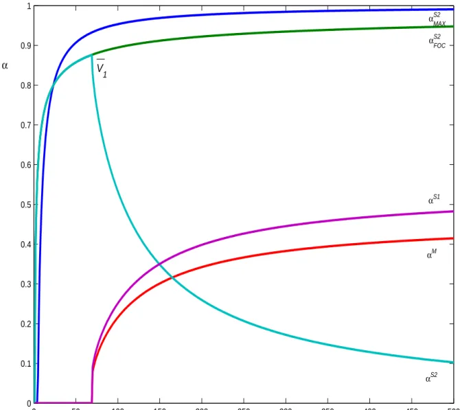
Figure 7 plots ownership shares against value at date 1 for the syndicate case when
I0, I1 = 50,50, σ = 0.4, θf = 1.8 and θg = 0.6, the same parameters used in Panel A of
Table 1. The top two lines show the syndicate’s maximum and optimal shares if the new investors were given free rein to maximize their NPV. The maximum share is irrelevant, as in Figure 4. The syndicate’s actual share equals its optimal share at the strike valueVS1 and then declines as V1 increases. The shares held by the entrepreneur and incumbent venture capitalist therefore increase as performance improves, consistent with the evidence in Kaplan and Stromberg (2003) and contrary to the pattern in the monopoly case, as plotted in Figure 4.
One might expect the better financing terms from the syndicate to decrease the strike value V1 from the monopoly case. But V1 is actually higher in the syndicate case — for example,V1is 84.9 in Figure 7 and 70.8 in Figure 4. This increase can be traced to the initial venture capitalist’s fixed original ownership share in the syndicate-financing case. When the original venture capitalist provides both rounds of financing, he picks the share at date 1 that is best for him at date 1. He may reduce his share to strengthen the entrepreneur’s incentives. Unlike the monopolist, the syndicate cannot reset the venture capitalist’s original share αC
0 and is there therefore faced with a free-riding incumbent. The syndicate has a smaller value pie to carve up, and a higher threshold for investment.
Thus the commitment to syndicate later-stage financing has two countervailing effects. The syndicate may require a higher threshold for investment, so that marginal projects will be rejected more often. On the other hand, syndication provides better incentives for the entrepreneur, so that low values off0V1 are less likely. Our numerical analysis will show that the second effect outweighs thefirst and that shifting from monopoly to syndication always adds value.
4.2
Renegotiation at date 1
Of course a low realization ofV1 could trigger a renegotiation between the incumbent and the entrepreneur to reset the incumbent’s initial share αC
0 before syndicate financing is sought. The incumbent can transfer ownership to the entrepreneur, retaining αC(R) < αC∗
0 , where
αC(R) denotes the incumbent’s renegotiated equity stake. The incumbent may be better
off accepting a reduced ownership share to improve the chance of success for low values of V1 or to increase continuation for V1 < V
S
1. By accepting a lower ownership share, the incumbent improves effort incentives for the entrepreneur to the point where enough extra value is added to support syndicate financing at NPV = 0. Of course the incumbent will give up as little as possible. In the worst renegotiation case, where V1 approaches a lower bound, the value of the incumbent’s shares approaches zero, just as in the monopoly case.
Renegotiation requires dilution of the incumbent venture capitalist’s ownership share. Dilution could happen in several ways. For example, the incumbent could provide bridge
financing on terms favorable to the entrepreneur. Dilution could also occur in a ”down round” — a round offinancing where new investors buy in at a price per share lower than in previous rounds. But our model says that a down round should dilute the entrepreneur less than the incumbent venture capitalist. The entrepreneur could be given additional shares or options, for example.
While renegotiation adds value ex post by improving effort and preserving access to
financing, the flexibility to reset shares at date 1 could introduce new problems. Suppose the initial venture capitalist sets αC
0 at a very high level, knowing that he can renegotiate down to the monopoly level at date 1, even when the realized valueV1 exceeds the syndicate strike value VS1.17 The entrepreneur would then cut back effort at dates 0 and 1 and reduce the value of the firm. This strategy amounts to a return to monopoly financing. It would reduce date-0 value to the venture capitalist as well as the entrepreneur.
Thus two conditions must hold in order for syndicate financing to work as we have described it. First, the initial venture capitalist has to commit at date 0 to syndicate at date 1. In practice this is not an explicit, formal commitment, but syndication is standard operating procedure. As part of the commitment, the initial venture capitalist has to limit his initial ownership shareαC
0 to its level in the syndicate case, so that he cannot start with a higher value and bargain down to the monopoly shareαC∗
1 at date 1. The commitment is in the venture capitalist’s interest, because it increases his ex ante value relative to the monopoly case. Second, the terms of financing in later rounds should be reasonably competitive. In practice they may not be perfectly competitive, but we believe the terms are materially better for the entrepreneur than the monopoly terms would be.
It turns out that opportunities for renegotiation are rare in our numerical experiments for the syndicate case. Therefore, incorporating the benefits of renegotiation would add relatively little to NPV at date 0. For example, including renegotiation gains would increase the NPVs reported in Table 1 by about 2% of the required total investment ofI0+I1 = 100.18 17The entrepreneur could retain the upside if she could bypass the incumbent venture capitalist and go
directly to the syndicate for financing. In practice the incumbent could block this end run by refusing to participate in the syndicate. The syndicate would assume that the incumbent has inside information, and would interpret the refusal to participate as bad news sufficient to deter their investment.
18We approximate renegotiation gains (holdingαC∗
4.3
E
ff
ort and exercise at date 0
At date 0, the venture capitalist sets αC
0 and the entrepreneur decides how much effort to exert. Given αC
0, the entrepreneur choosesx0 to maximize:
N P V0M(αC0) = max[0,max x0 (E0(N P V M 1 (x0(α C 0),α C 0)−g0(x0(α C 0)))] (11) The entrepreneur anticipates the syndicate’s share αS
1 as a function of date-1 value V1. For a given αC
0, date-1 syndicate financing will result in less dilution of her share than in the monopoly case, so she provides higher effort att= 0 as well as at t= 1. We cannot express NPV or effort in closed form, so we compute them numerically.
The venture capitalist anticipates the entrepreneur’s reaction when he sets αC
0. He must restrict his search to αC
0 ∈ 0,αC0(max) , where αC0(max) is determined by
E0(N P V1M(x0(α C 0(max)),α C 0(max))−g0(x0(α C 0(max)))) = 0 (12) This constraint rarely binds, since at the margin there is almost always value added by leaving positive value to the entrepreneur. Thus αC∗
0 is determined by αC0 = arg max αC 0∈(0,αC0(max)] E0(N P V1C(x0(α0C),αC0))−I0 (13) If N P VC 0 ≥0, investment proceeds.
Typical results for syndicate financing are shown in Table 1. Effort and value increase across the board, despite increases in the strike value VS1 from the monopoly case. We find that syndicate financing dominates monopoly financing with or without staged financing. Syndicatefinancing is better ex ante for the initial venture capitalist and also increases overall NPV. This is true for all parameter values, including values outside the range reported in Table 1. Yet there are still value losses relative to the first best.
4.4
The fully competitive case
Of coursefirst best is never attainable when the entrepreneur has to seek outside financing. Table 1 shows an alternative benchmark, the fully competitive case, in which all venture capital investors, including the initial investor at date 1, receiveN P V = 0. Fully competitive
financing gives an upper bound on the overall NPV when the entrepreneur has no money and has to share her marginal value added with outside investors. Solution procedures for the fully competitive case are identical to the syndication case, except thatαC
0 is set so that
N P VC
0 = 0.
Figure 8 shows date-1 ownership shares for the fully competitive case in the same format as the syndication case in Figure 7. Two things stand out. First, the entrepreneur’s share
at which the venture capitalist will start to reduce his share; (2) the new strike value and (3) the integral of NPV changes over this range. Only a small portion of the renegotiation gains come from more efficient continuation decisions (VS1(R)< V1< V
S
1). Most of the gains can be attributed to better effort incentives
(higherx1) in the region where the project continues regardless (V1> V
S
1). These gains further increase the
is higher and the initial venture capitalist’s lower than in Figure 7, because competitive
financing at date 0 gives relatively more shares to the entrepreneur. Both shares of course increase with the realized value V1. Second, the strike value V1 is lower in the competitive case, primarily because the entrepreneur’s initial effort is higher. Note also that the fully competitive NPVs, which go entirely to the entrepreneur, are less than in the first-best case, because the entrepreneur’s effort is lower. There is always some value loss when the entrepreneur has to share the marginal value added by her effort with outside investors.
4.5
Syndication with asymmetric information
So far we have assumed that the incoming syndicate investors and the incumbent venture capitalist are equally informed. Now we consider asymmetric information between the in-cumbent and new investors.
Both the incumbent and entrepreneur want the syndicate to perceive a high value V1. The more optimistic the syndicate, the higher the ownership shares retained by the incum-bent and entrepreneur. Reducing the syndicate’s share also increases the entrepreneur’s effort. Therefore, mere announcements of “great progress” or “high value” coming from the entrepreneur or incumbent are not credible.
Credibility may come from the incumbent’s fractional participation in date-1 financing. Suppose the incumbent invests βI1 and the outside syndicate the rest. What participation fraction β is consistent with truthful revelation of V1? If we could hold the entrepreneur’s effort constant, we could rely on Admati and Pfleiderer’s (1994) proof thatβ should befixed at the incumbent investor’s ownership share at date 0, that is, at αC
0. This fixed-fraction rule would remove any incentive for the incumbent to over-report V1. (The more he over-reports, the more he has to overpay for his new shares. Whenβ =αC
0, the amount overpaid cancels out any gain in the value of his existing shares.)19 The fixed-fraction rule would also insure optimal investment, since the incumbent’s share of date-1 investment exactly equals his share of thefinal payoffV2. Admati and Pfleiderer also show that no otherfinancing rule or procedure works in their setting.
Fixed-fraction financing does not induce truthful information revelation in our model, although a modified fixed-fractionfinancing works in some cases. The problem is the effect of the terms of date-1financing on the entrepreneur’s effort. Suppose the incumbent investor takes a fractionβ =αC
0 of date-1financing and then reports a value ˆV1that is higher than the true value V1. If the report is credible, the new shares are over-priced. The incumbent does not gain or lose from the mispricing, becauseβ =αC
0, but the entrepreneur gains on his old shares at the syndicate’s expense. Since the entrepreneur’s ownership share is higher than it would be under a truthful report, she exerts more effort, firm value increases, and both the entrepreneur and incumbent are better off. Therefore the incumbent will over-report.
A modified fixed-fraction rule can work, however, provided that β is set above αC0 and effort is not too sensitive to changes in the entrepreneur’s NPV at date 1. The required difference between β and αC
0 depends on the responsiveness of the entrepreneur’s effort to 19Thefixed-fraction rule would also remove any incentive to underreport. The more the incumbent
under-reports, the more he gains on the new shares. But the amount of profit made on the new shares is exactly offset by losses incurred on existing shares.
her ownership share. In many cases, a constant β set a few percentage points above αC0 removes the incentive to overreport over a wide range of V1 realizations. But this rule may break down as a general revelation mechanism in at least three ways.
First, whenV1is very low but exceedsV1, wefind situations where the requiredβ exceeds 1. This would make sense only if the new syndicate investors could short the company, so we must constrain β < 1. This outcome is common in our numerical results, because the incumbent’s initial share αC
0 is frequently above 85% - 90%, and in some of these cases the entrepreneur’s effort is very sensitive to the value of her stake in the firm. There is not much room forβ to increase between these starting points and a maximum level strictly less than 1. When β hits the maximum, the modifiedfixed fraction rule fails to induce truthful revelation.20
Second, the modifiedfixed fraction rule also fails whenV1 falls just belowV1. In this case the incumbent’s incentive to over-report becomes very strong, and only extremely high βs can discipline the incumbent to tell the truth. This problemflows from the discontinuity of the entrepreneur’s effort at the strike valueV1.Here the limit of β asV1 approachesV1 from below is infinity and nofixed-fraction rule works. This problem can be solved, however, if the incumbent and the entrepreneur renegotiate their ownership shares when V1 falls between the monopoly and syndicate strike values VC1and VS1. If the incumbent venture capitalist renegotiates, the lower strike value removes the discontinuity of effort. As the incumbent’s share declines, it is easier to find a β < 1 that works. The required β approaches 0 as V1 approachesVC1 and the incumbent’s share approaches zero.
The third problem arises at high levels of V1. Setting β > αC
0 gives the incumbent venture capitalist an incentive to under-report V1. The incumbent would gain more from underpricing the new shares and buying them cheaply than he would lose from dilution of his existing stake. Revelation works only if this incentive is offset by the impact on the entrepreneur’s effort. But as V1 and ˆV1 increase, effort becomes higher and less sensitive to the terms of financing. As effort tops out, the incentive to under-report takes over. This could be preventedlocally by allowingβto decrease with ˆV1, returning toβ=αC
0 at very high values. But then the almost-fixed fraction rule fails globally to induce truthful information revelation, because at lower V1 realizations he wants to over-report to these higher levels at which β =αC
0.
One possible solution, not fully explored here, is to introduce more complex contracts that allow signalling along two dimensions. For example, the incentive for the incumbent venture capitalist to under-report at high levels ofV1 could be offset by an incentive contract that grants the entrepreneur extra shares if the incumbent reports very high project value. With this additional provision in place, it should be possible to allow β to decrease with ˆV1, reaching β = αC
0 at high values of V1. This could be one justification for contingent share awards to the entrepreneurs, as observed in Kaplan and Stromberg (2003). Alternatively, the entrepreneur could be granted a series of stock options with increasing exercise prices, so that the entrepreneur’s final ownership share increases at high values of V2.
20This failure is less frequent if the entrepreneur has some personal wealth and can co-invest with the
venture capitalist at date 0. The coinvestment reduces the venture capitalist’s ownership share and provides more room forβ to increase to a maximum level strictly less than 1.
When the modifiedfixed fraction rule fails, the syndicate investors face the asymmetric information problem analyzed by Myers and Majluf (1984). In the special case of their model that is closest to our problem here, thefirm has no assets in place (no value in liquidation), so it goes ahead withfinancing on termsfixed by the new investors’ knowledge of the average value of V1. Syndicate investors would have to infer the average V1 from conditions at date 0, the entrepreneur’s effort functions and the entrepreneur’s and incumbent’s decision rules, given the anticipated terms of date-1 financing. But the investors do not know the true value V1, so their new financing is overpriced when V1 is low and underpriced when V1 is high. This leads to more effort when V1 is low and less when it is high, compared to the full-revelation case. But again there are problems. For example, ifV1 is high, the incumbent will be better off cancelling syndicate financing and providing the date-1 money directly. But if this is allowed, then the incumbent will have an incentive to claim a high valueV1 in order to reclaim monopoly power over the terms of financing. In addition, if the syndicate investors know less than the incumbent and the incumbent is free to finance the investment from his own pocket, then the incumbent will only raise syndicate financing if the syndicate is paying too much. Therefore a rational syndicate will not invest.21
Even if the revelation mechanism fails, there may be other ways to convey V1. The value of the incumbent investor’s reputation could generate truthful reports in a repeated game setting, for example. The syndicate usually includes other venture capitalists that the incumbent has worked with in the past and expects to work with in the future.
5
Summary of Numerical Results
Table 1 illustrates our main results. It shows surprisingly large value losses in most cases, relative to first-best. (For now ignore the debt-financing entries.) Value losses are greatest in the monopoly case where the initial venture capitalist provides all financing and dictates the terms of financing at date 1 as well as date 0. This does not imply that the venture capitalist extracts all value, leaving the entrepreneur with zero NPV. The venture capitalist wants to preserve the entrepreneur’s incentives to some extent. Nevertheless, the financing terms that maximize value for the venture capitalist usually leave the entrepreneur with a small minority slice of a diminished pie.
The problem with staged financing is that a monopolistic venture capitalist cannot com-mit not to hold up the entrepreneur ex post. Thus NPV can be higher and the initial venture capitalist better off if staged financing is abandoned and all financing is committed at date 0. Complete upfront financing is superior for all effort parameters (all values of θr =θf/θg)
when option value is relatively low, as it is for most of the range of standard deviations in Figure 5. Figure 6 shows that when the option value is high, staged financing is more efficient, despite the monopoly holdup problem.
Syndication of date-1 financing always makes both the entrepreneur and the initial ven-ture capitalist better off as long as the syndicate’s financing terms are reasonably competi-tive. This key result of our paper is evident in Table 1 and also holds generally. We believe that our syndicate case, in which the initial venture capitalist can set financing terms at date 0 but not date 1, is a good match to actual venture capital contracting. Of course we
observe syndication in practice, but that observation does not settle whether the terms of syndicatefinancing are competitive (NPV = 0) or monopolistic. Our analysis indicates that syndication terms are reasonably competitive. With monopoly financing terms at date 1, we find that the entrepreneur’s final ownership share is a decreasing function of firm value. With competitive terms, as in our syndication case, the entrepreneur’s share is an increasing function of value, consistent with practice (Kaplan and Stromberg (2003)).
The syndicate case is still inefficient, because it gives the initial venture capitalist the bargaining power to setfinancing terms at date 0. We believe that venture capitalists do have bargaining power and receive at least some (quasi) rents in earlyfinancing rounds. They have bargaining power because of experience and expertise, because of thefixed costs of setting up a venture capital partnership and because of the cost and delay that the entrepreneur would absorb in looking for another venture-capital investor. But there are obviously efficiency improvements if and as the terms of date-0 financing become more competitive. The fully competitive case shows the limit where the initial venture capitalist has no special bargaining power and just receives NPV = 0. Even the fully competitive case falls short of first best, however. The entrepreneur’s effort falls whenever outsidefinancing has to be raised, because the entrepreneur bears the full cost of effort, but has to share the marginal value added by effort with the outside investors.
Figure 9 summarizes value losses for the monopoly, no-staging, syndication and fully competitive cases over a wide range of the effort parameter θr. Value loss is defined as the
difference between NPV at date 0 andfirst-best NPV. The four panels correspond to panels A to D in Figure 1, except for the variation in θr. Figure 10 repeats Figure 9 for a more
profitable startup with V0 = 200.
The value losses plotted in Figure 9 increase rapidly with θr when θr is below 1.0, but
the losses are always less in the syndication case than in the monopoly cases. The losses in the syndicate case still appear economically significant, however. The only situations in which losses do not appear significant occur in the fully competitive case whenθr is above
2.0. High values for θr mean that effort generates value at relatively little cost, so that the
entrepreneur is willing to expend close tofirst-best effort in the fully competitive case, even though the marginal benefit of effort is shared with outside investors.
Value losses in the monopoly, no staging case increase as standard deviation is increased fromσ= 0.4 to 0.8. This is as expected, since staged financing is more valuable as volatility increases. But value losses may also increase with standard deviation in the monopoly and syndication cases, at least for the region whereθris about 1.0 and higher. We found this
sur-prising. Our original intuition was that increased uncertainty would enhance the optionality of investment and mitigate incentive problems. Instead it can make these problems worse, because more uncertainty can lead to lower initial effort.22 Compare the bottom-left and bottom-right panels in Figure 9, for example. The effects of volatility on effort and value can also be seen in panels E and F of Table 1. In the syndicate case, the value loss in panel
22When overall NPV is near zero, the entrepreneur’s effort x
0 increases rapidly with σ. The more
un-certainty, the greater chance that the entrepreneur’s call option will be in the money and the greater the marginal reward to effort. But as θr increases and NPV rises, effort eventually declines as σ increases, because the marginal impact of effort is less. The difference can be traced to the slope of the cumulative lognormal, which is lower at the mean whenσis high.
E, with σ = 0.


![Figure 3: Net Present Value at date 0 in the first-best scenario. N P V is shown across a range of standard deviation (σ ∈ [0.1, 1.2]) and effort return (θ f /θ g ∈ [1/11, 11]) parameters.](https://thumb-us.123doks.com/thumbv2/123dok_us/601883.2572053/50.918.162.774.379.941/figure-present-value-scenario-standard-deviation-effort-parameters.webp)