Outliers in semi-parametric Estimation of Treatment Effects

(1)

No. 17-20

2017

Outliers in semi-parametric Estimation of Treatment

Effects

(2)

Canavire-Outliers in semi-parametric Estimation of Treatment

E

↵

ects

Darwin Ugarte Ontiveros

⇤

, Gustavo Canavire-Bacarreza

†

and

Luis Castro Pe˜

narrieta

‡

Abstract

Average treatment e↵ects estimands can present significant bias under the presence of outliers. Moreover, outliers can be particularly hard to detect, creating bias and inconsistency in the semi-parametric ATE estimads. In this paper, we use Monte Carlo simulations to demonstrate that semi-parametric methods, such as matching, are biased in the presence of outliers. Bad and good leverage points outliers are considered. The bias arises because bad leverage points completely change the distribution of the metrics used to define counterfactuals. Whereas good leverage points increase the chance of breaking the common support condition and distort the balance of the covariates and which may push practitioners to misspecify the propensity score. We provide some clues to diagnose the presence of outliers and propose a reweighting estimator that is robust against outliers based on the Stahel-Donoho multivariate estimator of scale and location. An application of this estimator to LaLonde (1986) data allows us to explain the

Dehejia and Wahba (2002) and Smith and Todd(2005) debate on the inability of

matching estimators to deal with the evaluation problem. JEL: C21, C14, C52, C13

Keywords: Treatment e↵ects, Outliers, Propensity score, Mahalanobis dis-tance

⇤_{Universidad Privada Boliviana, La Paz, Bolivia, email: darwinugarte@lp.upb.edu corresponding}

author.

†_{Universidad EAFIT Medell´ın, Colombia and IZA, Bonn, Germany, email: gcanavir@eafit.edu.co}

(3)

1. Introduction

Parametric and nonparametric treatment e↵ects techniques are the workhorse tool when

examining the causal e↵ects of interventions, i.e., whether the outcome for an

obser-vation is a↵ected by the participation in a program or policy (treatment). Given the

impossibility of observing the same observation under the two potential states (partic-ipation and non-partic(partic-ipation), the use of counterfactual techniques is key when trying

to better identify causal e↵ects (Ashenfelter(1978);Ashenfelter and Card(1985);

Heck-man and Robb(1985);Heckman and Robb (1986)). As Bassi (1983),Bassi (1984) and

Hausman and Wise(1985) argue, counterfactual estimates are precise when using ran-domized experiments. Yet, when looking at non-ranran-domized experiments there are a number of assumptions, such as unconfoundedness, exogeneity, ignorability, or selection

on observables, that should be considered before estimating the true e↵ect, or to get

close to that of a randomized experiment1 _Imbens ₍₂₀₀₄_).

While there are several assumptions one needs to consider when identifying

treat-ment e↵ects (see King et al. (2017)), one that has been overlooked in the existing

literature is the existence of outliers (both, on the outcome or on the covariates). We

followJarrell(1994),Rasmussen(1988), andStevens(1984) by defining outliers as those

few observations that behave atypically from the bulk of the data, and are therefore much larger or smaller than the values of the remaining observations in the sample. One of the main problems caused by outliers is that they may bias or modify estimates

of priority interest, and in our case, the treatment e↵ect (see some discussion in

Ras-mussen (1988); Schwager and Margolin (1982); and Zimmerman (1994)). In addition, they may increase the variance and reduce in consequence the power of methods, espe-cially those within the non-parametric family. If non-randomly distributed, they may reduce normality, violating in the multivariate analyses the assumption of sphericity

and multivariate normality, as noted byOsborne and Overbay (2004).

To the best of our knowledge, the e↵ects of outliers in the estimation of

semi-parametric treatment e↵ects have not yet been analyzed in the literature. The only

reference is Imbens (2004), who directly associates outlying values in the covariates

to a lack of overlap. Imbens (2004) argues that outlier observations will present

esti-mates of the probability of receiving treatment close to 0 or 1, and therefore, methods dealing with limited overlap can produce estimates approximately unchanged in bias and precision. As shown in this paper, this intuition is valid only for outliers what

are considered good leverage points. Moreover, Imbens (2004) expresses that treated

observations with outlying values may lead to biased covariate matching estimates since these observations would be matched to inappropriate controls. Control observations

with outlying covariate values, on the other hand, will likely have little e↵ect on the

es-timates of average treatment e↵ect for the treated, since such observations are unlikely

1 _{For a complete discussion and examples on the relationship between randomized and}

non-randomized experiments and their bias, see LaLonde (1986), Heckman et al. (1997a) and Heckman

(4)

to be used as matches. We provide evidence for this intuition.

Thus, in this paper, the relative performance of leading semi-parametric estimators

of average treatment e↵ects in the presence of outliers is examined. Three types of

outliers are considered: bad leverage points, good leverage points and vertical outliers. The analysis considers outliers located in the treatment group, the control group, and in

both groups. We focus on (i) the e↵ect of these outliers in the estimation of the metric,

propensity score and Mahalanobis distance, (ii) the e↵ect of these contaminated (by

outliers) metrics in the matching procedure when finding counterfactuals, and (iii) the

e↵ect of these matches in the estimation of the average treatment e↵ect on the treated

(TOT).

Using Monte Carlo simulations, we show that the semi-parametric estimators of

average treatment e↵ects produce biased estimations in the presence of outliers. A

summary of our findings is as follows: First, bad leverage points bias estimations of

av-erage treatment e↵ects. The bias emerges as this type of outlier completely changes the

distribution of the metrics used to define good counterfactuals, and therefore changes the matches that had initially been undertaken, assigning as matches observations with

very di↵erent characteristics. This e↵ect is independent of the location of the outlier

observation. Second, good leverage points in the treatment sample slightly bias

estima-tions of average treatment e↵ects, as they increase the chance of infringing the overlap

condition. Third, good leverage points in the control sample do not a↵ect the

estima-tion of treatment e↵ects, as they are unlikely to be used as matches. Fourth, these

outliers distort the balance of the covariates criterion used to specify the propensity score. Fifth, vertical outliers in the outcome variable greatly bias estimations of

aver-age treatment e↵ects. Sixth, good leverage points can be identified visually by looking

at the overlap plot. Bad leverage points, however, are masked in the estimation of the metric and are, as a consequence, practically impossible to be identified unless a for-mal outlier identification method is implemented. Therefore, we suggest a re-weighting

treatment e↵ect estimator that is robust against outliers based on theStahel(1981) and

Donoho (1982) estimator of scale and location, proposed in the literature by Verardi et al.(2012). What we suggest is thus to identify all types of outliers in the data by this

method, and again estimate treatment e↵ects, down-weighting the importance of

out-liers; this is a one-step reweighted treatment e↵ect estimator. Monte Carlo simulations

support the utility of this tool to overcome the e↵ects of outliers in the semi-parametric

estimation of treatment e↵ects.

An application of this estimator toLaLonde(1986) data allows us to understand the

failure ofDehejia and Wahba (1999), Dehejia and Wahba (2002) matching estimations

to overcome LaLonde’s critique of non-experimental estimators. We show that the

crit-icism bySmith and Todd (2005) aboutDehejia and Wahba(1999),Dehejia and Wahba

(2002) large bias when considering LaLonde’s full sample can be explained by the

pres-ence of outliers in the data. When down-weighting the e↵ect of these outliers, Dehejia

and Wahba(1999), Dehejia and Wahba (2002) matching estimations approximate the

(5)

This paper is structured as follows. Section2briefly reviews the literature. Section3

defines the balancing hypothesis, the semi-parametric estimators, the types of outliers considered, as well as the Stahel-Donoho estimation of location and scatter tool to

detect outliers. In Section4, the data generating process (DGP) is characterized. The

analysis of the e↵ects of outliers is presented in Section 5. An application to LaLonde’s

data is presented in Section 6. And in Section 7, we conclude.

2. A Brief Review of the Literature

Blundell and Costa Dias(2000) argue that the fundamental problem of causal inference arises because we can never observe both states (participation and non-participation)

for the same observation at the same time, i.e., one of the states is counterfactual2 _.

Thus, some assumptions are required to produce a more precise counterfactual and to

estimate the actual causal e↵ect. Within this framework, pure randomized controlled

experiments are seen as desirable, especially for discovery and evidence for policy3 _.

However, in the absence of experimental information, which is largely the case,

alter-native identification strategies for observational data are required4 _.

Many studies in the literature have shown that a comparison of the results of stud-ies that used experimental data with those that used non-experimental data provide important advances to assess methods where it is impossible to work with experimental data. The results found in the experimental and non-experimental data were relatively

close (seeLaLonde (1986); Heckman et al.(1997a); Heckman et al. (1997b); or Ferraro

et al.(2015)).

In recent decades, there has been increasing interest in the econometric and

sta-tistical analysis of causal e↵ects. Various methods for estimating average treatment

e↵ects for a binary treatment under di↵erent sets of assumptions have been suggested

(Imbens and Wooldridge (2009)). One strand of this literature has developed

statisti-cal techniques for estimating treatment e↵ects under the assumption that by adjusting

treatment and control groups for di↵erences in observed covariates, all biases in

com-parisons between treated and control observations are removed. The assumption is diversely referred to as unconfoundedness, exogeneity, ignorability, or selection on

ob-servables (seeImbens (2004) for a discussion). Under this assumption, nonparametric

methods, such as matching, which have wide recognition for non-experimental

statis-tical evaluation (see Heckman et al. (1997a)), have become a valued tool for recent

evaluations of treatments in observational studies, as presented by Smith and Todd

(2005) andDehejia(2005). These methods select treated and comparison observations

2_{There are many references in literature that document this evaluation problem, including}

Ashen-felter(1978),Ashenfelter and Card(1985),Heckman and Robb(1985), andHeckman and Robb(1986).

3_{For a discussion on the goods and bads of experimentation see} _{Deaton and Cartwright}_(2016).

4 _{Some of the more relevant evaluation methods are the pure randomized social experiment,}

pre-sented byBassi(1983),Bassi(1984) andHausman and Wise(1985), who based their contributions on

(6)

with similar characteristics in terms of covariates to predict the counterfactual out-come. This is done by defining similarity in terms of a metric: Mahalanobis distance

values (Rubin(1980)) or propensity score values (Rosenbaum and Rubin(1983)). Some

combination of both metrics has also been suggested (Zhao(2004)).

As argued earlier, an often overlooked, but important problem in econometric and statistical analysis is the existence of outliers. Outliers may bias and even modify point

and distributional estimates, such as those produced when looking at treatment e↵ects.

Moreover, they increase the variance and reduce the power of the estimands, as argued byRasmussen(1988),Schwager and Margolin(1982),Zimmerman(1994), andOsborne and Overbay (2004).

Various methods for identifying outliers have been proposed based on di↵erent

methodologies, like statistical reasoning (Hadi et al. (2009)), distances (Angiulli and

Pizzuti(2002);Knorr et al.(2000); and Orair et al.(2010)), or densities (Breunig et al.

(2000)); (De Vries et al.(2010) andKeller et al.(2012)). But the issue is not completely

solved, and in some methodologies, such as causal inference, this issue may become cru-cial. The problem increases as outliers often do not show up by simple visual inspection or by univariate analysis, and in the case several outliers are grouped close together in a region of the sample space, far away from the bulk of the data, they may mask one

another (seeRousseeuw and Van Zomeren (1990)).

In regression analysis, Rousseeuw and Leroy (2005) define three types of outliers:

Good Leverage Points (GLP) are observations (Xi, Yi) whose Xi deviates from the ma-jority in the X-dimension and follows the linear pattern of the mama-jority. If, on the other

hand, the observations do not follow this linear pattern and theirXi are outlying in the

X-dimension, they are Bad Leverage Points (BLP). Finally, if the observations deviate

from the linear pattern but theirXibelong to the majority in the X-dimension they are

calledVertical Outliers (VO). Statistical estimations based on a sample including these

extreme observations may dissent heavily from the true estimation (seeRuppert(1987),

Hampel et al.(2011), Maronna et al.(2006), andAndersen (2008) for an assessment of estimation methods that are robust against outliers.

To illustrate the problem, in a labor market setting, as the one inAshenfelter(1978)

andAshenfelter and Card (1985), consider a case in which the path of the data clearly shows that highly educated people attend a training program, while uneducated individ-uals do not. Now assume that there are a small number of individindivid-uals without schooling who are participating in the program, and a small number of educated individuals who are not in the training program, while having similar remaining characteristics. These peculiar individuals may constitute bad leverage points in the treatment and control sample, respectively. Enrolled individuals with an outstanding level of education may represent good leverage points. This small number of individuals, who may genuinely belong to the sample or may be errors from the data encoding process, may have a

large influence on the treatment e↵ect estimation and drive the conclusion about the

(7)

(2009) and Heckman and Vytlacil (2005). The problem considered in this paper is that as semi-parametric techniques, matching methods rely on a parametric estima-tion of the metrics (propensity score and Mahalanobis distance) used to define and compare observations with similar characteristics in terms of covariates, while the re-lationship between the outcome variables and the metric is nonparametric. Therefore, the presence of multivariate outliers in the dataset can strongly distort estimations of

the metrics and lead to unreliable treatment e↵ect estimations. According to

informa-tion presented by Rousseeuw and Van Zomeren (1990), vertical outliers can also bias

the nonparametric relationship between the metric and the outcome by distorting the average outcome in the observed or counterfactual group. Moreover, these distortions, by the presence of multivariate outliers in the dataset, can conflict the balance of the

covariates when specifying the propensity score, as in Dehejia (2005). This has

prac-tical implications. When choosing the variables to specify the propensity score it may not be necessary to discard troublesome but relevant variables from a theoretical point

of view or generate senseless interactions or nonlinearities. It might be sufficient to

discard troublesome observations (outliers). That is, outliers can push practitioners to unnecessarily misspecify the propensity score.

3. Framework

(i) Matching methods: To lay out the setup, we rest on the traditional potential outcome

approach developed by Rubin (1974), which views causal e↵ects as comparisons of

potential outcomes defined on the same unit. In the potential outcome framework,

each observation i = 1. . . n has two potential responses (Y0

i , Yi1) for a treatment. Yi1

is the outcome if observation i is treated (treatment group), and Y0

i is the outcome if

observation i is not treated (control group). Each observation is exposed to a single

treatment: Ti = 0 if the observation receives the control treatment and Ti = 1 if the

observation receives the active treatment. In addition, each observation has a vector

of characteristics Xi that are not a↵ected by the treatment (usually referred to as

covariates, pre-treatment variables or exogenous variables). For each observation, it is

therefore observed the triplet (Yi;Ti ₂_{0,1_};Xi), whereYi is the realized outcome:Yi =

TiY1

i + (1 Ti)Yi0. Unfortunately, we never observe both Yi0 and Yi1 simultaneously,

so eitherY0

i orYi1 is missing for each observation. To estimate the average treatment

e↵ect, we thus need to estimate the unobserved potential outcome for each observation

in the sample.

Non-parametric techniques, such as matching, impute the non-observable potential

outcome (Y0

i ) by finding for each observation, other observations whose covariates are

similar but who were not exposed to the treatment. To ensure that the matching

esti-mators identify and consistently estimate the treatment e↵ect of interest the following

set of assumptions has been found useful: (i) that assignment to treatment is

indepen-dent of the outcomes, conditional on the covariates, (Y0

i , Yi1)?Ti|Xi, usually referred

(8)

assignment is bounded away from zero and one,& < P(Xi)_⌘P(Ti = 1_|Xi)<1 &, for some& >0, also known as strict overlap assumption. SeeImbens(2004) for a discussion

of these assumptions. In this paper, we focus on the average treatment e↵ect on the

treated⌧ =E[Y1

i Yi0|Xi, Ti = 1].

As mentioned above, matching estimators impute the missing potential outcome by using outcomes for observations with similar values for the covariates. However, when there are many covariates it is impractical to match them directly because of the curse of dimensionality. Therefore, it is necessary to map the multiple covariates into a balancing

metricm(Xi), a scalar, that can measure the closeness of two observations. This metric

is defined byRosenbaum and Rubin(1983) as a function of the observed covariates such

that the conditional distribution of Xi given m(Xi) is the same for the treated and

comparison groups. The most often used metrics in the literature are theMahalanobis

distance, D(Xi)⌘ ||X||s = (X0SX)1/2, which is the vector norm with positive definite

matrixS corresponding to the inverse of the sample covariance matrix of the covariates,

and thePropensity Score,P(Xi)_⌘P(Ti = 1_|Xi), which is the predicted probability for

Ti = 1 given the covariatesXi. Then, conditioning on covariatesD(Xi), or conditioning

on the propensity scoreP(Xi), will both make the distribution of the covariates in the

treated group the same as the distribution of the covariates in the control group.5 _{This is}

the balancing hypothesis, and it can be represented asTi ?Xi|m(Xi). If it is achieved,

observations with the same metric must have the same distribution of observable (and unobservable) characteristics, independent of treatment status. The achievement of a

balanced model depends on the specification used to estimate the metric, see Dehejia

and Wahba (2002) for a discussion on specification issues.

A variety of matching estimators has been proposed for estimating the

counterfac-tual mean. Following the approach of Busso et al. (2009), the out-of-sample

fore-cast for treated unit l based only on control units j can be represented as ˆY0

i =

P

j(1 Ti)YjWl,j/

P

j(1 Tj)Wl,j, where Wl,j provides the distance between

observa-tionslandj in terms of the metricm(Xi) ={D(Xi), P(Xi)}. The matching estimators

di↵er in the weight Wl,j used to estimate the counterfactual ˆY0

i .

In this paper, we will focus on those estimators that, supported by recent evidence, show good finite-sample performance and have established asymptotic properties (see

Fr¨olich (2004), Busso et al. (2009), and Busso et al. (2014)). We thus examine the

e↵ect of outliers on the following matching estimators: propensity score pair matching,

propensity score local linear ridge matching, bias-corrected covariate matching, and

reweighting based on propensity score. Busso et al. (2009) show that pair matching

exhibits good performance in terms of bias, but with higher variance in small samples. Local linear ridge matching and reweighting perform well in terms of bias and variance

oncen= 500. In addition, Busso et al.(2014) showed that the bias-corrected covariate

estimator is more e↵ective in settings with poor overlap. Large sample properties

5_See_Rubin_(1980),_{Rosenbaum and Rubin}_{(1983), and recently}_Zhao_{(2004) for a comparison and}

(9)

for these estimators have been approached by Heckman et al. (1997a), Hirano et al.

(2003), and Abadie and Imbens (2006). Pair matching proceeds by finding for each

treated observation a control observation with a very similar value of m(Xi), that is,

it sets Wl,j = 1 if the control observationj has the metric closest to that of treatment

observation l, and sets Wl,j = 0 otherwise. Local linear ridge matching (Seifert and

Gasser (2000)), is a variation of kernel matching based on a local linear regression

estimator that adds a ridge term to the denominator of the weight Wl,j in order to

stabilize the local linear estimator. To estimate it we consider the Epanechnikov kernel. The bandwidth is selected by a simple leave-one-out cross-validation procedure with

the search grid h = 0.01p1.2g 2 _for _g _{= 1}_,₂_{, . . . ,}₁ _following _Fr¨olich ₍₂₀₀₄_{). The}

bias-corrected covariate matching estimator attempts to remove the bias in the nearest neighbor covariate matching estimator coming from inexact matching in finite samples.

It adjusts the di↵erence within the matches for the di↵erences in their covariate values.

This adjustment is based on regression functions (see Abadie and Imbens (2011)) for

details. Finally, in addition to these matching estimators, we consider the normalized

reweighting estimator, where Wl,j =P(Xj)/(1 P(Xj)) and the sum of the weights is

1.

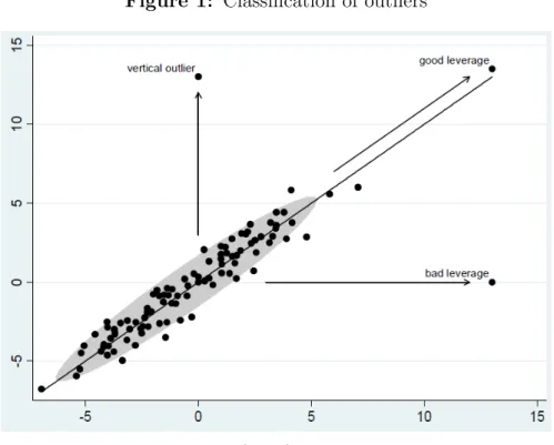
(ii) Classification of outliers: Semi-parametric estimators of treatment e↵ects may

be very sensitive to outliers. As explained by Rousseeuw and Leroy (2005), in

cross-section regression analysis, a source of bias may come from three kinds of contamination

sources: in the error term (vertical outliers) and the explanatory variables (two kinds

of leverage points: good and bad). Vertical outliers are those observations that are far away from the bulk of the data in the Y-dimension, i.e., outlying in the dependent variable, but present a behavior similar to the group in the X-dimension, i.e., are not

outlying in the design space. Vertical outliers can a↵ect the value of the coefficients in

regression analysis and bias them downward or upward. Good leverage points (GLP) are observations that are far from the bulk of the data in the X-dimension, i.e., outlying in the regressors but are not located far from the regression line. Their existence in

regression analysis does not a↵ect the estimators but can a↵ect the inference and induce

the estimator to not be rejected as statistically significant. Finally, bad leverage points (BLP) are observations that are far from the bulk of the data in the X-dimension

and are located far from the regression line. They a↵ect the coefficients in regression

analysis. A diagram to help distinguish these types of outliers can be found in Verardi

and Croux (2009) (see figure1).

(iii) A reweighted estimator: What we suggest for coping with the e↵ect of these outliers is to identify all types of outliers in the data and down-weight their importance

(a one-step reweighted treatment e↵ect estimator). Here we suggest following Verardi

et al. (2012) and use as an outlier identification tool the projection-based method of

Stahel(1981) and Donoho (1982), hereafter called SD.

An interesting feature of this projection-based tool is that contrary to what occurs in other multivariate tools to identify outliers, like the minimum covariance determinant estimator (MCD) or the S-estimator of multivariate location and scatter (Smultiv),

(10)

Figure 1: Classification of outliers

Source: Verardi and Croux (2009).

dummies are not a problem. This feature is important as we are considering treatment

e↵ects and the main variable of interest is a dummy (Ti). Moreover, the presence

of categorical explanatory variables in treatment e↵ects empirical research is highly

frequent. The advantage of the SD tool is its geometric approach: in regression analysis, even if one variable is always seen as dependent on others, geometrically there is no

di↵erence between explanatory and dependent variables and the data is thus a set of

points (Yi, Ti, Xi) in a (p+ 1) dimensional space. Thus, an outlier can be seen as a point

that lies far away from the bulk of the data in any direction. Note that the utility of this

tool is not restricted to treatment e↵ect models and it can be implemented to detect

outliers in a broad range of models (seeVerardi et al. (2012) for some applications).

The Stahel(1981) and Donoho (1982) estimation of location and scatter (SD) con-sists of calculating the outlyingness of each point by projecting the data cloud unidi-mensionally in all possible directions and estimating the distance from each observation to the center of each projection. The degree of outlyingness is defined as the maximal distance that is obtained when considering all possible projections. Since this

outly-ingness distance ( ) is distributed as p 2

p, we can choose a quantile above which we

consider an observation as being outlying (we consider here the 95th percentile)6 _{. For}

specific details about this method seeVerardi et al.(2012), andMaronna et al. (2006).

Once the outliers have been identified, a one-step reweighted treatment e↵ect

(11)

tor can be implemented. In this paper, we use the most drastic weighting scheme that consists of awarding a weight of zero to any outlying observation. Once the importance awarded to outliers is down-weighted, the bias coming from outliers will disappear.

4. Monte Carlo Setup

The data generating process (DGP) is as follows:

Ti = 1(T_i⇤ >0)

T_i⇤ =f(Xi) +µi

Yi =⌧Ti+ Xi+"i

Where µi _⇠N(0,1) and "i ⇠N(0,1) are independent of Xi ⇠ N(0,1) and of each

other. The sample sizes aren ={500,1500} and the number of covariates p={2,10}.

2000 replications are performed. The experiment is designed to detect the e↵ect of

outliers on the performance of various estimators. A benchmark case is considered, which sidesteps important issues that may constitute a source of bias in the estimation, like poor overlap in the metrics between treatment and control units, misspecification of the metric, etc. The idea is to see how outliers can move us away from this benchmark case. The design of the Monte Carlo study consists of two parts, (i) the functional form and distribution of the metric in the treated and control groups, and (ii) the kind of outlier contaminating the data.

Initially, following Fr¨olich (2004), the propensity score is specified as a linear

func-tion f(Xi) =↵+ Xi and through the choice of di↵erent values for ↵, di↵erent ratios

of control to treated observations are generated. The parameter ↵ manages the

aver-age value of the propensity score and the number of treated relative to the number of

controls in the sample. Then, in the first design (forp= 2),f(Xi) = 0.5X1+ 0.5X2 the

population mean of the propensity score is 0.5. That is, the expected ratio of control

to treated observations is 1 : 1. In the second design, f(Xi) = 0.65 + 0.5X1 + 0.5X2

the ratio is 7 : 3 (the pool of control observations is large), and in the third design,

f(Xi) = 0.65 + 0.5X1+ 0.5X2, the ratio is 3 : 7 (the treated greatly exceed the

con-trols). We consider these designs, as during the estimation of the counterfactual mean,

more precisely during the matching step. The e↵ects of outliers in the treated or control

groups could be o↵set by the number of observations in this group. The fourth design

considers the equal size of the treatment and control groups, but a nonlinear

specifica-tion of the propensity score on the covariate of interest: f(Xi) = 0.5X1+0.15X12+0.5X2.

In addition,Yi = 0.15 +Ti+ 0.5X1+ 0.5X2, that is, the true treatment e↵ect is one. In

the DGP we do not consider di↵erent functional forms for the conditional expectation

function of Yi given Ti. Results from Fr¨olich (2004) suggest that when the matching

estimator takes the average, the e↵ects of these nonlinearities may disappear.

As mentioned before, the strict overlap assumption is always satisfied in these

(12)

-consistency of semi-parametric treatment e↵ect estimators. Busso et al. (2009) show

that with Xi and µi distributed standard normal for the linear specification of f(Xi).

This assumption is achieved when _{| |} _ 1. The intuition behind this result is that

when approaches 1, an increasing mass of observations have propensity scores near 0

and 1. This leads to fewer and fewer comparable observations and an e↵ective sample

size smaller thann. This is important because it implies potentially poor finite sample

properties of semi-parametric estimators in contexts where is near 1. In our designs,

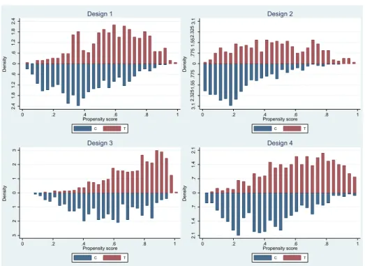
we set = 0.5 for the linear and nonlinear functions of f(Xi). The overlap plots

sup-port the achievement of the strict overlap assumption for these cases, as they do not

display mass near the corners. This can be observed in figure2, where the conditional

density of the propensity score given treatment status (overlap plot) for the four designs considered in the Monte Carlo simulations are displayed.

The second part of the design concerns the type of contamination in the sample. To grasp the influence of the outliers we will consider three contamination setups inspired by Croux and Haesbroeck (2003). The first is called clean with no contamination.

In the second, called mild, 5% of X1 are awarded a value 1.5pp units larger than

what the DGP would suggest. The third is a setup called severe in which 5% ofX1 are

awarded a value 5ppunits larger than the DGP would suggest. Moreover, as mentioned

above, three types of outliers are recognized in the literature: bad leverage points, good leverage points, and vertical outliers. Then, nine additional scenarios can be considered in the analysis depending on the localization of these outliers in the sample. That is, three types of outliers can be located in the treatment sample (T), in the control sample (C), and in both groups (T and C). Therefore, we assess the relative performance of the

estimators described in last section in a total of seventy-two di↵erent contexts. These

di↵erent contexts are characterized by combinations of four designs forf(Xi), two types

of contamination (mild and severe), and three types of outliers located in treatment, control and in both groups, respectively.

(13)

Figure 2: Overlap plots for the designs 3 2 1 0 1 2 3 D e nsi ty 0 .2 .4 .6 .8 1 Propensity score C T Design 3 2. 1 1. 4 .7 0 .7 1. 4 2. 1 D e nsi ty 0 .2 .4 .6 .8 1 Propensity score C T Design 4 2. 4 1. 8 1. 2 .6 0 .6 1. 2 1. 8 2. 4 D e nsi ty 0 .2 .4 .6 .8 1 Propensity score C T Design 1 3. 1 2. 32 51. 55 .7 75 0 .7 75 1. 55 2. 32 53. 1 D e nsi ty 0 .2 .4 .6 .8 1 Propensity score C T Design 2

Source: Authors calculations.

5. The e↵ect of outliers in the estimation of treatment e↵ects

This section analyses the e↵ect of outliers in the estimation of treatment e↵ects through

the illustration of two simple cases, the e↵ect of outliers in the estimation of the metrics

used to define similarity, and the e↵ect of these (spurious) metrics in the assignment of

matches when finding counterfactuals, is described.

5.1 The e↵ect of outliers in the metrics

a) The distribution of the Propensity Score in presence of outliers

Then, an artificial dataset is used to illustrate the e↵ect of outliers in the distribution

of the metrics in the presence of bad and good leverage points. 1500 observations were generated following the first design of our DGP. The original distribution of the propensity score by treatment status (overlap plot) corresponds to the top left graph

of figure 2. The graphs on the top of figure 3 applies to the overlap plots for the

same sample but with five percent of the data contaminated by bad leverage points

in the treatment sample, in the control, and in both samples respectively. As can be seen, the propensity score is now clearly less spread out than the one obtained with the original data in both treatment and control groups. That is, the distribution of

(14)

corresponds to the values of the original propensity score, whereas the cloud of points corresponds to the values of the propensity score in the presence of bad leverage points in the treatment sample, in the control, and in both samples respectively. They show

huge di↵erences in the values of the propensity score between the original and the

contaminated sample. These changes in the distribution of the propensity score due to some outliers suggest, in addition, that the propensity score masks bad leverage points,

as they cannot be distinguished in the data. Note that these e↵ects are identical if we

consider bad leverage points in the control sample, or in both treatment and control groups.

Figure 3: E↵ect of bad leverage points on the propensity score

2. 9 2. 17 51. 45 .7 25 0 .7 25 1. 45 2. 17 52. 9 D e nsi ty 0 .2 .4 .6 .8 1 Propensity score C T A: Pr(T) with BLP in T 3. 2 2. 4 1. 6 .8 0 .8 1. 6 2. 4 3. 2 D e nsi ty 0 .2 .4 .6 .8 1 Propensity score C T B: Pr(T) with BLP in C 3. 1 2. 32 51. 55 .7 75 0 .7 75 1. 55 2. 32 53. 1 D e nsi ty 0 .2 .4 .6 .8 1 Propensity score C T C: Pr(T) with BLP in T and C 0 .2 .4 .6 .8 1 Pro p en si ty sco re 0 .2 .4 .6 .8 1 Propensity score Clean Pr(T) Pr(T) with BLP in T

A.1: Comparison of Pr(T)s, case BLP in T

0 .2 .4 .6 .8 1 Pro p en si ty sco re 0 .2 .4 .6 .8 1 Propensity score Clean Pr(T) Pr(T) with BLP in C B.1: Comparison of Pr(T)s, case BLP in C 0 .2 .4 .6 .8 1 Pro p en si ty sco re 0 .2 .4 .6 .8 1 Propensity score

Clean Pr(T) Pr(T) with BLP in T and C

C.1: Comparison of Pr(T)s, case BLP in T and C

On the top of figure 4, the distribution of the propensity score by treatment status

in the presence of good leverage points in the treatment sample, in the control, and in both samples, is displayed. On the bottom of Figure 4, the straight line corresponds to the values of the original propensity score, whereas the cloud of points corresponds to the values of the propensity score in the presence of good leverage points. As can

be observed, a di↵erence of bad leverage points, the so called good leverage points do

not change completely the distribution of the propensity score and can be identified visually.

A theoretical explanation for these results can be found in Croux et al.(2002), who

showed that the non-robustness against outliers of the maximum likelihood estimator

in binary models is characterized because it does not explode to infinity as in ordinary

(15)

Figure 4: E↵ect of good leverage points on the propensity score 3. 4 2. 55 1. 7 .8 5 0 .8 5 1. 7 2. 55 3. 4 D e nsi ty 0 .2 .4 .6 .8 1 Propensity score C T A: Pr(T) with GLP in T 3. 5 2. 62 5 1. 75 .8 75 0 .8 75 1. 75 2. 62 53. 5 D e nsi ty 0 .2 .4 .6 .8 1 Propensity score C T B: Pr(T) with GLP in C 2. 2 1. 65 1. 1 .5 5 0 .5 5 1. 1 1. 65 2. 2 D e nsi ty 0 .2 .4 .6 .8 1 Propensity score C T C: Pr(T) with GLP in T and C 0 .2 .4 .6 .8 1 Pro p en si ty sco re 0 .2 .4 .6 .8 1 Propensity score Clean Pr(T) Pr(T) with GLP in T

A.1: Compatison of Pr(T)s, case GLP in T

0 .2 .4 .6 .8 1 Pro p en si ty sco re 0 .2 .4 .6 .8 1 Propensity score Clean Pr(T) Pr(T) with GLP in C B.1: Comparison of Pr(T)s, case GLP in C 0 .2 .4 .6 .8 1 Pro p en si ty sco re 0 .2 .4 .6 .8 1 Propensity score

Clean Pr(T) Pr(T) with GLP in T and C

C.1: Comparison of Pr(T)s, case GLP in T and C

set. That is, given the maximum likelihood estimator of a binary dependent variable,

ˆ_{M L} _{= arg max}_{Log L}_{( ;}_Xn₎

where Log L( ;Xn) is the log-likelihood function calculated in . Croux et al. (2002)

showed two important facts: (i) good leverage points (glp) do not perturb the fit

ob-tained by the ML procedure, that is _{M L}glp _! M L. However, as displayed in figure4, the

fitted probabilities of these outlying observations will be close to zero or one. Here, it

can lead to unstable estimates of the treatment e↵ects as the support (or overlap)

con-dition is not met. (ii) In presence of bad leverage points (blp), the ML-estimator never

explodes, asymptotically it tends to zero. That is, _{M L}blp ! 0. In addition, following

Fr¨olich (2004) andKhan and Tamer (2010), coefficients close to zero in the estimation of the propensity score will then reduce the variability of the propensity score, as these

coefficients ( ) determine the spread of the propensity score. Therefore, the presence

of bad leverage points in the data will always narrow the distribution of the propensity

score, as found in figure3. As is showed below, this tightness in the distribution of the

propensity score may increase the chance of matching observations with very di↵erent

characteristics.

The e↵ect of these distortions in the density of the propensity score in the matching

process and in the treatment e↵ect estimation is discussed in next sections.

b) The distribution of the Mahalanobis distance in presence of outliers

In figure 5, the straight line corresponds to the values of the Mahalanobis distance

(16)

of this metric in the presence of bad and good leverage points in the treatment sam-ple, in the control, and in both samples, respectively. Three remarks can arise from these graphs. First, bad and good leverage points present an atypical behavior in the sense that they display larger distances. Since Mahalanobis distances are computed individually for each observation, bad and good leverage points present bigger values, whereas remaining observations stay relatively stable. This behavior is independent of the location of the outlier. Second, bad and good leverage points slightly change the distribution of the distances, the stability of the not contaminated observations is relative in the sense that all distances are standardized by the sample covariance matrix

of the covariates (S 1_{), which is in turn based on biased measures (by the outliers) of}

the averages and variances in the sample. Third, concluding that observations with large distances can directly be called outliers may be fallacious, just in the sense that to be called outliers these distances need to be estimated by a procedure that is robust against outliers in order to provide reliable measures for the recognition of outliers.

This is the masking e↵ect, see Rousseeuw and Van Zomeren(1990). Single extreme

ob-servations or groups of obob-servations, departing from the main data structure, can have

a severe influence on this distance measure because the covariance (S 1_{) is estimated}

in a non-robust manner; that is, it is biased.

Figure 5: E↵ect of bad and good leverage points on the Mahalanobis distance

5

0 1 2 3 4 Ma h al an ob is di st a nce s 0 2 4 6 8 10 Mahalanobis distances Clean M.D. M.D. with BLP in T A: Distances with BLP in T 0 1 2 3 4 Ma h al an ob is di st a nce s 0 5 10 Mahalanobis distances Clean M.D. M.D. with BLP in C B: Distances with BLP in C 0 1 2 3 4 Ma h al an ob is di st a nce s 0 2 4 6 8 10 Mahalanobis distances Clean M.D. M.D. with BLP in T and C C: Distances with BLP in T and C

0 1 2 3 Ma h al an ob is di st a nce s 0 5 10 15 20 Mahalanobis distances Clean M.D. M.D. with GLP in T and C F: Distances with GLP in T and C

0 1 2 3 Ma h al an ob is di st a nce s 0 5 10 15 20 Mahalanobis distances Clean M.D. M.D. with GLP in T D: Distances with GLP in T 0 1 2 3 Ma h al an ob is di st a nce s 0 5 10 15 Mahalanobis distances Clean M.D. M.D. with GLP in C E: Distances with GLP in C

5.2 A description of the matching process in the presence of outliers

In this section, a small, artificial dataset is used to illustrate the e↵ect of outliers in

(17)

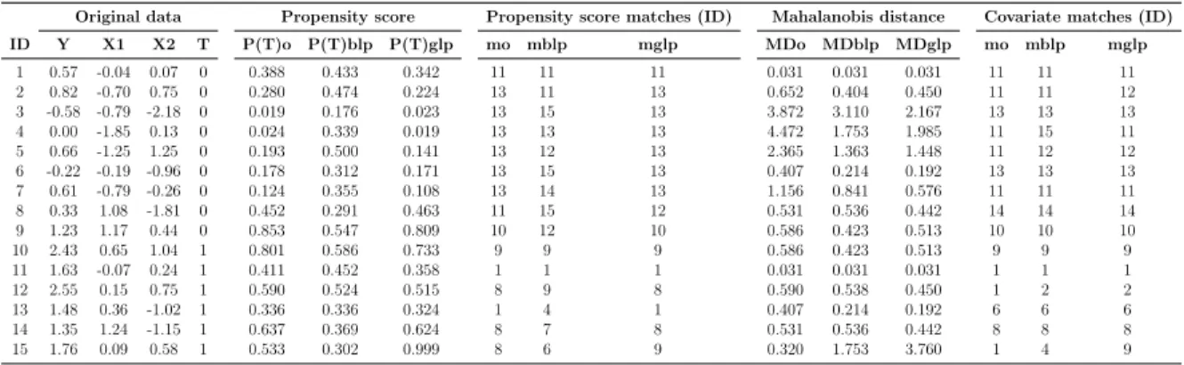
observations for the first design of our DGP are generated. These variables are presented

in the first four columns of table1. The exercises consist of substituting the value of one

observation in one covariate, seeing in detail its e↵ect on the matches assigned. One bad

and one good leverage point is generated by moving the value of the last observation of

X1by +2.5

p

2 and by 2.5p2, respectively. Columns five to seven of table1present the

propensity score estimated with the original and contaminated data, respectively. As observed, the distribution of the propensity score with bad leverage points completely changes. Observations 5 and 9, for example, change their probability of participating in the program from 0.19 to 0.5 and from 0.85 to 0.54, respectively. The distribution of the propensity score with good leverage points holds the same path, but the probability of the outlier observation jumps from 0.3 to 0.99. Columns eight to ten show the

consequent e↵ect of the variation in this metric on the matches assigned to generate

the counterfactuals (by using the nearest neighbor criteria)7 _{. Consider observation}

13, for example. Initially, it is presented as a counterfactual observation 1, but due to the presence of the bad leverage point, the nearest observation now corresponds with observation 4. The matches assigned in the presence of good leverage points are the same (with the exception of the observation with an outlier). Columns eleven to thirteen

show the behavior of the Mahalanobis distance. As can be observed, the e↵ect of the

bad and good leverage point on this metric is similar. In both cases, the distribution changes slightly and the distances of the outlier observations increase abruptly. In

the last three columns, we can see the e↵ect on the assignation of counterfactuals.

Observation 12, for example, is originally matched to observation 1. But in presence of the outlier it is matched to observation 2.

Table 1: E↵ect of a bad leverage point on the matching assignment

Original data Propensity score Propensity score matches (ID) Mahalanobis distance Covariate matches (ID) ID Y X1 X2 T P(T)o P(T)blp P(T)glp mo mblp mglp MDo MDblp MDglp mo mblp mglp 1 0.57 -0.04 0.07 0 0.388 0.433 0.342 11 11 11 0.031 0.031 0.031 11 11 11 2 0.82 -0.70 0.75 0 0.280 0.474 0.224 13 11 13 0.652 0.404 0.450 11 11 12 3 -0.58 -0.79 -2.18 0 0.019 0.176 0.023 13 15 13 3.872 3.110 2.167 13 13 13 4 0.00 -1.85 0.13 0 0.024 0.339 0.019 13 13 13 4.472 1.753 1.985 11 15 11 5 0.66 -1.25 1.25 0 0.193 0.500 0.141 13 12 13 2.365 1.363 1.448 11 12 12 6 -0.22 -0.19 -0.96 0 0.178 0.312 0.171 13 15 13 0.407 0.214 0.192 13 13 13 7 0.61 -0.79 -0.26 0 0.124 0.355 0.108 13 14 13 1.156 0.841 0.576 11 11 11 8 0.33 1.08 -1.81 0 0.452 0.291 0.463 11 15 12 0.531 0.536 0.442 14 14 14 9 1.23 1.17 0.44 0 0.853 0.547 0.809 10 12 10 0.586 0.423 0.513 10 10 10 10 2.43 0.65 1.04 1 0.801 0.586 0.733 9 9 9 0.586 0.423 0.513 9 9 9 11 1.63 -0.07 0.24 1 0.411 0.452 0.358 1 1 1 0.031 0.031 0.031 1 1 1 12 2.55 0.15 0.75 1 0.590 0.524 0.515 8 9 8 0.590 0.538 0.450 1 2 2 13 1.48 0.36 -1.02 1 0.336 0.336 0.324 1 4 1 0.407 0.214 0.192 6 6 6 14 1.35 1.24 -1.15 1 0.637 0.369 0.624 8 7 8 0.531 0.536 0.442 8 8 8 15 1.76 0.09 0.58 1 0.533 0.302 0.999 8 6 9 0.320 1.753 3.760 1 4 9

For a proper estimation of the unobserved potential outcomes, we want to compare treated and control groups that are as similar as possible. These simple illustrations explain that extreme values can easily distort the metrics used to define similarity and

thus may bias the estimation of treatment e↵ects by making the groups very di↵erent.

7_{Note that although we searched for the single closest match, as will be shown below, the illustration}

(18)

That is, the prediction of ˆY0

l for the treated group is made using information from

observations that are di↵erent from themselves. In the next section, we present evidence

about the e↵ects on the treatment e↵ect estimations.

5.3 Monte Carlo Results

In this section the results of the Monte Carlo simulations are examined. The aim is to

analyze the e↵ect of outliers in the estimation of treatment e↵ects in di↵erent scenarios.

Table 2examines the performance in the estimation of the average treatment e↵ect

on the treated of the four selected estimators for the first design of our DGP. It presents the bias and mean squared error, scaled by 1000, from 2000 replications. The sample

size (n) is 1500 and the number of covariatesp= 2. The severe and mild contamination

setups are considered in panel A and panel B, respectively. Columns correspond to the type of outlier and rows to the estimators. Column one, called clean, involves the no-contamination scenario. Columns two to four contain bad leverage points in the treatment, control, and both groups simultaneously, respectively. Similarly, columns five to seven consider good leverage points, whereas columns eight to ten correspond to vertical outliers in the treatment, control, and in both samples, respectively.

Table 2: Simulated bias and MSE of treatment e↵ect estimations

in the presence of outliers

Panel A: Severe contamination Bad Leverage Points Good Leverage Points Vertical outliers in Y Estimators: Clean in T in C in T and C in T in C in T and C in T in C in T and C

BIAS Pair Matching 6,7 388,8 387,6 388,6 124,6 6,4 58,4 723,6 705,3 16,0 Ridge M. Epan 7,2 391,8 389,4 390,7 117,2 2,7 58,1 724,3 712,8 7,0 IPW 4,2 387,2 383,0 385,4 41,3 8,3 2,2 722,3 715,3 5,0 Covariate M. BC 1,0 358,7 1,3 182,1 358,5 0,8 181,6 717,2 716,8 1,6 MSE Pair Matching 0,8 152,6 151,7 152,4 18,2 0,9 4,9 524,7 525,3 16,7 Ridge M. Epan 0,6 154,1 152,3 153,3 15,5 0,6 4,4 525,4 523,9 10,0 IPW 3,9 150,6 147,4 149,3 3,8 2,6 3,2 524,9 529,3 13,1 Covariate M. BC 0,6 130,0 0,7 33,8 131,5 0,7 34,3 515,3 538,0 14,2

Rejection Balance of Cov 10,0% 99,6% 90,0% 18,4% 41,2% 49,8% 50,8% Panel B: Mild contamination

Rejection Balance of Cov 11,8% 85,4% 75,6% 50,0% 27,2% 12,4% 14,0%

(19)

all the estimators we considered perform well, which is in accordance with recent

ev-idence provided by Busso et al. (2009), and Busso et al. (2014). The bias-corrected

covariate matching ofAbadie and Imbens(2011) has the smallest bias, followed by the

local linear ridge propensity score matching and the reweighting estimator based on the propensity score. Second, in the presence of bad leverage points, all the estimators present a considerable bias. For the propensity score matching methods, the size of the bias is generally the same, independent of the location of the outlier. This is expected since, as explained in the last section, the complete distribution of the metrics changes when bad leverage points exist in the data. The spread of the metrics decreases and observations that initially presented larger (lower) values of the metric may now match with observations that initially had lower (larger) values. Therefore, for pair matching the spurious metric will match inappropriate controls. For local linear ridge

match-ing the weightsWl,j, which are a function (kernel) of the di↵erences in the propensity

score, will decrease notably. And in the case of the reweighted estimator, some control observations will receive higher weights as their propensity score values are higher than those values from the original data, and some will receive lower weights (as the weights are normalized to sum up to one). For the covariate matching estimator, treatment

observations with bad leverage points bias the treatment e↵ect estimation as the

dis-tribution of the distances changes completely. Moreover, outlier observations present larger values for the metric and are matched to inappropriate controls. Bad leverage

points in the control sample have little e↵ect on the estimates of average treatment

ef-fect for the treated as the distribution of the distances changes completely, but outlier observations are less likely to be considered as counterfactuals.

Third, good leverage points in the treatment sample also bias the treatment e↵ect

estimations of the propensity score matching estimators. Good leverage points in the treatment sample have estimates of the probability of receiving treatment close to 1. These treated observations with outlying values lack suitable controls against which to compare them. This violates the overlap assumption and therefore increases the likelihood of biasing the matching estimations. In the case of the reweighted estimator, the unbiasedness is explained as just the outliers receive higher weights, while remain-ing observations present almost the same weight (slightly modified by a normalization procedure). Moreover, good leverage points in the treatment group greatly bias the

covariate matching estimator. This e↵ect, which is similar to those coming from bad

leverage points, is explained as these outlying observations have larger values for the metric and are therefore matched to inappropriate controls.

Fourth, good leverage points in the control sample do not a↵ect matching methods.

For the propensity score matching estimators, the values of the propensity score for

the outliers are close to 0 and these observations would cause little difficulty because

they are unlikely to be used as matches. For the reweighted estimator, these outlying observations would get close to zero weight. For the covariate matching estimators,

good leverage points in the control sample have little e↵ect on the estimations, as

(20)

leverage points are presented in both samples, treatment e↵ect estimations are biased. This bias probably comes from the outliers in the treatment group.

Sixth, vertical outliers bias the treatment e↵ect estimations. This bias is easy to

understand since extreme values in the outcomes,Y1

i orYi0, will move the average values

toward them in their respective groups, independent of the estimator used to match

the observations. Seventh, the immediate e↵ect of outliers is to reject the balancing

hypothesis.

Finally, table 3 analyses the e↵ectiveness of the reweighted treatment e↵ect

esti-mator based on the projection-based identification of outliers’ tool (SD). The aim of this set of simulations is to check how the outlier identification tool we propose and the subsequent reweighted estimator behaves with these models. The structure of table

3 is similar to that of table 1. The results suggest two main conclusions. First, the

SD algorithm performs well in a scenario without outliers. That is, applying the SD

algorithm does not influence the estimation of treatment e↵ects in case no outliers are

present in the data. Similar results were obtained when applying this tool to other

estimators (see Verardi et al. (2012)). Second, as expected, the reweighted estimators

we propose resist the presence of outliers and lead to estimations that are similar to those obtained with the clean sample in all contamination scenarios.

It is worth mentioning that the general conclusions obtained with designs two to

four are very similar, although the e↵ect of outliers is slightly smaller in design four.

Similarly, the results obtained when consideringn= 500, or when using ten covariates

(p= 10) are practically identical to those presented above. These results are available

(21)

Table 3: Simulated bias and MSE of the reweighted treatment e↵ect estimations based on the SD method

Panel A: Severe contamination Bad Leverage Points Good Leverage Points Vertical outliers in Y Estimators: Clean in T in C in T and C in T in C in T and C in T in C in T and C

Panel B: Mild contamination

6. An outlier analysis of the Dehejia-Wahba (2002) and Smith-Todd (2005) debate

A debate has arisen, starting with LaLonde (1986), which evaluates the performance

of non-experimental estimators using experimental data as a benchmark. Dehejia and

Wahba(1999) andDehejia and Wahba(2002) findings of low bias from applying

propen-sity score matching toLaLonde(1986) data contributed strongly to the popularity and

implementation of this method in the empirical literature - suggesting it as a good way

to deal with the selection problem. Smith and Todd(2005) (hereafter called ST), using

the same data and model specification as Dehejia and Wahba (hereafter called DW), suggest that the low bias estimates presented in DW are quite sensitive to the sample and the propensity score specification, thus claiming that matching methods do not

solve the evaluation problem when applied to LaLonde’s data.8

In this section, we suggest that the DW propensity score model’s inability to

ap-8_{DW applied propensity score matching estimators to a subsample of the same experimental data}

from the National Supported Work (NSW) Demonstration, and the same non-experimental data from the Current Population Survey (CPS) and the Panel Study of Income Dynamics (PSID), analyzed by LaLonde (1986). ST re-estimated DW’s model to three samples: LaLonde’s full sample, DW’s

sub-sample, and a third sub-sample (ST-sample). SeeDehejia and Wahba(1999),Dehejia and Wahba

(22)

proximate the experimental treatment e↵ect when applied to LaLonde’s full sample

is managed by the existence of outliers in the data. When down-weighting the e↵ect

of these outliers the DW propensity score model presents low bias. Note that we do not interpret these results as proof that propensity score matching solves the selection problem since the third subsample (ST sample) continues reporting biased matching

estimates after down-weighting the e↵ect of outliers. Moreover, this data allows us to

highlight the role of outliers when performing the balance of the covariate checking

in the specification of the propensity score. Dehejia (2005), in a reply to ST, argues

that a di↵erent specification should be selected for each treatment group - comparison

group combination, and that ST misapplied the specifications that DW selected for their samples to samples for which the specifications were not necessarily appropriate

“as covariates are not balanced”. Dehejia(2005) states that with suitable specifications

selected for these alternative samples, with covariates well balanced, accurate estimates can be obtained. Remember that in estimating the propensity score the specification is determined by the need to condition fully on the observable characteristics that make up the assignment mechanism. That is, that the distribution of the covariates should be approximately the same across the treated and comparison groups once the propensity score is controlled for. Then the covariates can be defined as well-balanced when the

di↵erences in propensity score for treated and comparison observations are insignificant

(see the appendix in Dehejia and Wahba(2002)).

ST suggests that matching fails to overcome LaLonde’s critique of non-experimental

estimators, as it presents large bias when applied to LaLonde’s full sample, while

De-hejia(2005) states that this failing comes from the use of a wrong specification of the propensity score for that sample (as the covariates are not balanced). In this section, we suggest that matching has low bias when applied to LaLonde’s full sample and that the specification of the propensity score employed was not wrong, it was that the sample was contaminated with outliers. These outliers initially distorted the balance of the

covariates, leadingDehejia (2005) to conclude that the specification was not right, and

also biased the estimation of the treatment e↵ect, causing ST to conclude that

match-ing does not approximate the experimental treatment e↵ect when applied to LaLonde’s

full sample. These conclusions can be found in table 4, which shows the propensity

score nearest neighbor treatment e↵ect estimations (TOT) for DW’s subsample and

LaLonde’s full sample.9 _{The dependent variable is real income in 1978. Columns one}

and two describe the sample, that is, the comparison and treatment groups, respectively.

Column three reports the experimental treatment e↵ect for each sample. Column four

presents the treatment e↵ect estimations for each sample. The specification of the

propensity score corresponds to that used by Dehejia and Wahba(1999), Dehejia and

Wahba (2002), and Smith and Todd (2005).10 _{Column five reports the treatment} ef-fect estimations for each sample by using the same specification as in column four and

9_{I would like to thank professor Smith for kindly sharing his data with us.}

10_{The specification for the PSID comparison group is: age, age squared, schooling, schooling squared,}

no high school degree, married, black, Hispanic, real earnings in 1974, real earnings in 1974 squared, real earnings in 1975, real earnings in 1975 squared, dummy zero earning in 1974, dummy zero earning

(23)

down-weighting the e↵ect of outliers identified by the Stahel-Donoho method described

in section 2. Three remarks arise from table 4. First, the treatment e↵ect estimations

for LaLonde’s sample (in column four) are highly biased compared with the true e↵ects

(column three), as shown by DW. Second, once the outliers are identified and their

importance down-weighted, the treatment e↵ect estimations improve meaningfully in

terms of bias, and the matching estimations approximate the experimental treatment

e↵ect when considering LaLonde’s full sample. And third, once the e↵ect of outliers

is down-weighted, the propensity score specifications now balance the covariates suc-cessfully. This has practical implications, as when choosing the variables to specify the propensity score it might not be necessary to discard troublesome variables that may be relevant from a theoretical point of view, or to generate senseless interactions or

non-linearities. It might be sufficient to discard troublesome observations (outliers). That

is, outliers can push practitioners to unnecessarily misspecify the propensity score.

Table 4: Treatment e↵ect estimations of the LaLonde and DW samples

Experimental Estimated Estimated

Comparison group Treatment group TOT TOT SD-TOT

PSID [2490 obs] LaLonde [297 obs] 886 -28 (1070) 670 (964)

PSID [2490 obs] Dehejia-Wahba [185 obs] 1794 2317 (1266) 1203(1299)

CPS [15992 obs] LaLonde [297 obs] 886 -351 (810) 736 (889)

CPS [15992 obs] Dehejia-Wahba [185 obs] 1794 731 (882) 1587 (854)

7. Conclusions

Assessing the impact of any intervention requires making an inference about the out-comes that would have been observed for program participants had they not partici-pated. Matching estimators impute the missing outcome by finding other observations in the data whose covariates are similar but who were exposed to the other treatment. The criteria used to define similar observations, the metrics, is parametrically estimated by using the predicted probability of treatment (propensity score), or the standardized distance on the covariates (Mahalanobis distance).

Moreover, it is known that in statistical analysis the values of a few observations (outliers) often behave atypically from the bulk of the data. These atypical few obser-vations can easily drive the estimations in empirical research.

In this paper, the relative performance of leading semi-parametric estimators of

average treatment e↵ects in the presence of outliers is examined. It is found that: (i)

in 1975, Hispanic* dummy zero earning in 1974. The specification for the CPS group is: age, age squared, age cubed, schooling, schooling squared, no high school degree, married, black, Hispanic, real earnings in 1974, real earnings in 1975, dummy zero earning in 1974, dummy zero earning in 1975, schooling* real earnings in 1974.

(24)

bad leverage points bias estimations of average treatment e↵ects. This type of outlier changes completely the distribution of the metrics used to define good counterfactuals and, therefore, changes the matches that had initially been undertaken, assigning as

matches observations with very di↵erent characteristics. (ii) Good leverage points in the

treatment sample slightly bias estimations of average treatment e↵ects and they increase

the chance of infringing the overlap condition. (iii) Good leverage points in the control

sample do not a↵ect the estimation of treatment e↵ects as they are unlikely to be used as

matches. (iv) These outliers break the balancing criterion used to specify the propensity score. (v) Vertical outliers in the outcome variable greatly bias estimations of average

treatment e↵ects. (vi) Good leverage points can be identified visually by looking at

the overlap plot. Bad leverage points, however, are masked in the estimation of the

metric and are difficult to identify. (vii) TheStahel(1981) andDonoho(1982) estimator

of scale and location, proposed by Verardi et al. (2012) as a tool to identify outliers

is e↵ective for this purpose. The proposed reweighted estimator produces unbiased

matching estimators in the presence of outliers. (vii) An application of this estimator to

LaLonde(1986) data allows us to understand the failure ofDehejia and Wahba(1999), and Dehejia and Wahba(2002) matching estimations to produce unbiased estimations when considering LaLonde’s full sample. This failure can be explained by the presence of outliers in the data.

References

Abadie, A. and Imbens, G. W. (2006). Large sample properties of matching estimators

for average treatment e↵ects. Econometrica, 74(1):235–267.

Abadie, A. and Imbens, G. W. (2011). Bias-corrected matching estimators for average

treatment e↵ects. Journal of Business & Economic Statistics, 29(1):1–11.

Andersen, R. (2008). Modern methods for robust regression. Number 152. Sage.

Angiulli, F. and Pizzuti, C. (2002). Fast outlier detection in high dimensional spaces. In European Conference on Principles of Data Mining and Knowledge Discovery, pages 15–27. Springer.

Ashenfelter, O. (1978). Estimating the e↵ect of training programs on earnings. The

Review of Economics and Statistics, pages 47–57.

Ashenfelter, O. and Card, D. (1985). Using the Longitudinal Structure of Earnings

to Estimate the E↵ect of Training Programs. The Review of Economics and

Statistics, 67(4):648–660.

Bassi, L. J. (1983). The E↵ect of CETA on the Postprogram Earnings of Participants.

The Journal of Human Resources, 18(4):539–556.

Bassi, L. J. (1984). Estimating the e↵ect of training programs with non-random

selec-tion. The Review of Economics and Statistics, pages 36–43.

Blundell, R. and Costa Dias, M. (2000). Evaluation methods for non-experimental data.

Fiscal Studies, 21(4):427–468.

(25)

density-based local outliers. In ACM sigmod record, volume 29, pages 93–104. ACM.

Busso, M., DiNardo, J., and McCrary, J. (2009). Finite sample properties of

semi-parametric estimators of average treatment e↵ects. forthcoming in the Journal of

Business and Economic Statistics.

Busso, M., DiNardo, J., and McCrary, J. (2014). New evidence on the finite sample

properties of propensity score reweighting and matching estimators. The Review

of Economics and Statistics, 96(5):885–897.

Cochran, W. G. and Rubin, D. B. (1973). Controlling bias in observational studies: A

review. Sankhy¯a: The Indian Journal of Statistics, Series A, pages 417–446.

Croux, C., Flandre, C., and Haesbroeck, G. (2002). The breakdown behavior of the

maximum likelihood estimator in the logistic regression model. Statistics &

Prob-ability Letters, 60(4):377–386.

Croux, C. and Haesbroeck, G. (2003). Implementing the Bianco and Yohai estimator

for logistic regression. Computational statistics & data analysis, 44(1):273–295.

De Vries, T., Chawla, S., and Houle, M. E. (2010). Finding local anomalies in very

high dimensional space. In Data Mining (ICDM), 2010 IEEE 10th International

Conference on, pages 128–137. IEEE.

Deaton, A. and Cartwright, N. (2016). Understanding and misunderstanding random-ized controlled trials. Technical report, National Bureau of Economic Research. Dehejia, R. (2005). Practical propensity score matching: a reply to Smith and Todd.

Journal of Econometrics, 125(1):355–364.

Dehejia, R. H. and Wahba, S. (1999). Causal e↵ects in nonexperimental studies:

Reeval-uating the evaluation of training programs. Journal of the American Statistical

Association, 94(448):1053–1062.

Dehejia, R. H. and Wahba, S. (2002). Propensity score-matching methods for

nonexper-imental causal studies. The Review of Economics and Statistics, 84(1):151–161.

Donoho, D. L. (1982). Breakdown properties of multivariate location estimators. Tech-nical report, TechTech-nical report, Harvard University, Boston.

Ferraro, P. J., Hanauer, M. M., Miteva, D. A., Nelson, J. L., Pattanayak, S. K., Nolte, C., and Sims, K. R. (2015). Estimating the impacts of conservation on ecosystem

services and poverty by integrating modeling and evaluation. Proceedings of the

National Academy of Sciences, 112(24):7420–7425.

Fisher, R. A. (1951). The design of experiments. Oliver And Boyd; Edinburgh; London,

6th edition.

Fr¨olich, M. (2004). Finite-sample properties of propensity-score matching and weighting

estimators. The Review of Economics and Statistics, 86(1):77–90.

Hadi, A. S., Imon, A. H. M., and Werner, M. (2009). Detection of outliers. Wiley

Interdisciplinary Reviews: Computational Statistics, 1(1):57–70.

Hampel, F. R., Ronchetti, E. M., Rousseeuw, P. J., and Stahel, W. A. (2011). Robust

statistics: the approach based on influence functions, volume 114. John Wiley & Sons.

(26)

Press for National Bureau of Economic Research, Chicago.

Heckman, J. J., Ichimura, H., and Todd, P. E. (1997a). Matching as an econometric

evaluation estimator: Evidence from evaluating a job training programme. The

Review of Economic Studies, 64(4):605–654.

Heckman, J. J. and Robb, R. (1985). Alternative methods for evaluating the impact of

interventions: An overview. Journal of Econometrics, 30(1):239–267.

Heckman, J. J. and Robb, R. (1986). Alternative methods for solving the problem of

selection bias in evaluating the impact of treatments on outcomes. In Drawing

inferences from self-selected samples, pages 63–107. Springer.

Heckman, J. J., Smith, J., and Clements, N. (1997b). Making the most out of gramme evaluations and social experiments: Accounting for heterogeneity in

pro-gramme impacts. The Review of Economic Studies, 64(4):487–535.

Heckman, J. J. and Vytlacil, E. (2005). Structural equations, treatment e↵ects, and

econometric policy evaluation1. Econometrica, 73(3):669–738.

Hirano, K., Imbens, G. W., and Ridder, G. (2003). Efficient estimation of average

treatment e↵ects using the estimated propensity score. Econometrica, 71(4):1161–

1189.

Imbens, G. W. (2004). Nonparametric estimation of average treatment e↵ects under

exogeneity: A review. The Review of Economics and Statistics, 86(1):4–29.

Imbens, G. W. and Wooldridge, J. M. (2009). Recent developments in the econometrics

of program evaluation. Journal of Economic Literature, 47(1):5–86.

Jarrell, M. G. (1994). A comparison of two procedures, the Mahalanobis distance and

the Andrews-Pregibon statistic, for identifying multivariate outliers. Research in

the Schools, 1(1):49–58.

Keller, F., Muller, E., and Bohm, K. (2012). HiCS: High contrast subspaces for

density-based outlier ranking. InData Engineering (ICDE), 2012 IEEE 28th International

Conference on, pages 1037–1048. IEEE.

Khan, S. and Tamer, E. (2010). Irregular identification, support conditions, and inverse

weight estimation. Econometrica, 78(6):2021–2042.

Khandker, S. R., Koolwal, G. B., and Samad, H. A. (2009). Handbook on impact

evaluation: quantitative methods and practices. World Bank Publications.

King, G., Lucas, C., and Nielsen, R. A. (2017). The Balance-Sample Size Frontier in

Matching Methods for Causal Inference. American Journal of Political Science,

61(2):473–489.

Knorr, E. M., Ng, R. T., and Tucakov, V. (2000). Distance-based outliers: algorithms

and applications. The VLDB Journal—The International Journal on Very Large

Data Bases, 8(3-4):237–253.

LaLonde, R. J. (1986). Evaluating the econometric evaluations of training programs

with experimental data. The American Economic Review, pages 604–620.

Maronna, R., Martin, R. D., and Yohai, V. (2006). Robust statistics. John Wiley &

Sons, Chichester. ISBN.

Orair, G. H., Teixeira, C. H., Meira Jr, W., Wang, Y., and Parthasarathy, S. (2010).