A multigrid approach to SDP relaxations of sparse polynomial optimization problems

(1)

A multigrid approach to SDP

relaxations of sparse polynomial

optimization problems

Juan S. Campos Salazar

Department of Computing

Imperial College London

Submitted in partial fulfilment of the requirements for the degree of Doctor of Philosophy in Computing of Imperial College and

(2)

DECLARATION

I, Juan S. Campos Salazar, declare that this thesis, and the research to which it refers, are the product of my own work, and that any ideas or quotations from the work of other people, published or otherwise, are fully acknowledged in accordance with the standard referencing practices of the discipline.

(3)

c

The copyright of this thesis rests with the author and is made available under a Creative Commons Attribution Non-Commercial No Derivatives licence. Researchers are free to copy, distribute or transmit the thesis on the condition that they attribute it, that they do not use it for commercial purposes and that they do not alter, transform or build upon it. For any reuse or redistribution, researchers must make clear to others the licence terms of this work.

(4)

A multigrid approach to SDP relaxations of sparse polynomial

optimization problems

Abstract

We propose two multigrid approaches for the global optimization of polynomial op-timization problems. In our first contribution we consider problems that arise from the discretization of infinite dimensional optimization problems, such as PDE optimiza-tion problems, boundary value problems and some global optimizaoptimiza-tion applicaoptimiza-tions. In many of these applications, the level of discretization can be used to obtain a hierarchy of optimization models that captures the underlying infinite dimensional problem at different degrees of fidelity. This approach, inspired by multigrid methods, has been successfully used for decades to solve large systems of linear equations. However, it has not been adapted to SDP relaxations of polynomial optimization problems. The main difficulty is that the geometric information between grids is lost when the original problem is approximated via an SDP relaxation. Despite the loss of geometric infor-mation, we show how a multigrid approach can be applied by developing prolongation operators to relate the primal and dual variables of the SDP relaxation between lower and higher levels in the hierarchy of discretizations. We develop sufficient conditions for the operators to be useful in applications. Our conditions are easy to verify in prac-tice, and we discuss how they can be used to reduce the complexity of infeasible interior

(5)

point methods. Following the same reasoning, the second approach does not assume any particular structure of the underlying polynomial problem, but instead considers the hierarchy of sparse SDP relaxations that can be obtained for any unconstrained polynomial optimizations problem with structured sparsity. Prolongation operators are defined for this type of hierarchy, and theoretical results that show their usefulness are proved. Our preliminary results highlight two promising advantages of following a multigrid approach in contrast with a pure interior point method: the percentage of problems that can be solved to a high accuracy is much higher, and the time necessary to find a solution can be reduced significantly, especially for large scale problems.

(6)

(7)

ACKNOWLEDGMENTS

I want to thank Imperial College London for funding my PhD during these 4 years, as well as my supervisor Panos Parpas and the Computational Optimisation Group.

(8)

LIST OF FIGURES

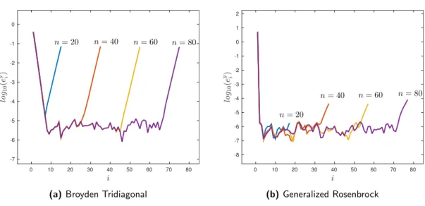
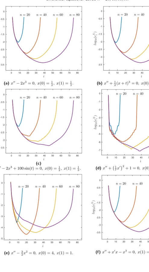
4.1 Logarithm ofey_i =yn α−−y_αn α∈∪i_k+₌p_i−1Bk (i= 2,3, . . . , n−2p+ 2) for

global optimization functions. Levels n= 20,40,60,80. . . 94

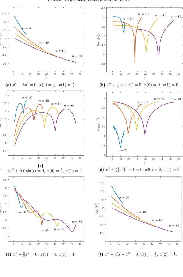
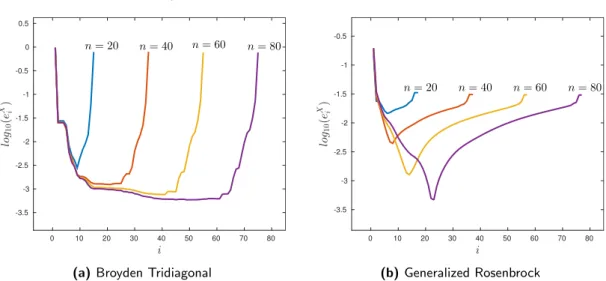
4.2 Logarithm of ey_i =

y_αn−−y_αn

α∈∪i_k+₌p_i−1Bk (i = 2,3, . . . , n−2p+ 2)

for the non-linear differential equations. Levels n= 20,40,60,80. . . 95

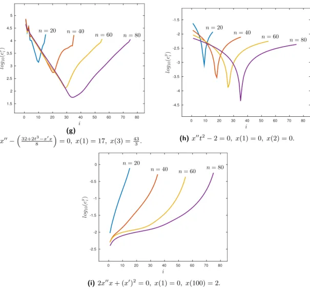
4.2 (Continued) Logarithm ofey_i =yn

α−−yn_α

α∈∪i_k+₌p_i−1Bk(i= 2,3, . . . , n−

2p+ 2) for the non-linear differential equations. Levelsn= 20,40,60,80. 96

4.3 Logarithm of eX i = max kXn l −Xln−1k i+p−1 l=i (i= 2,3, . . . , n−2p+ 2)

for the global optimization functions. Levels n= 20,40,60,80.. . . 97

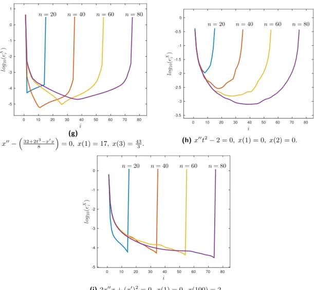
4.4 Logarithm of eX i = max kXn l −Xln−1k i+p−1 l=i (i= 2,3, . . . , n−2p+ 2)

for the non-linear differential equations. Levels n= 20,40,60,80. . . 98

4.4 (Continued) Logarithm ofeX_i = maxkX_ln−X_ln₋₁k i+p−1

l=i (i= 2,3, . . . , n−

2p+ 2) for the non-linear differential equations. Levelsn= 20,40,60,80. 99

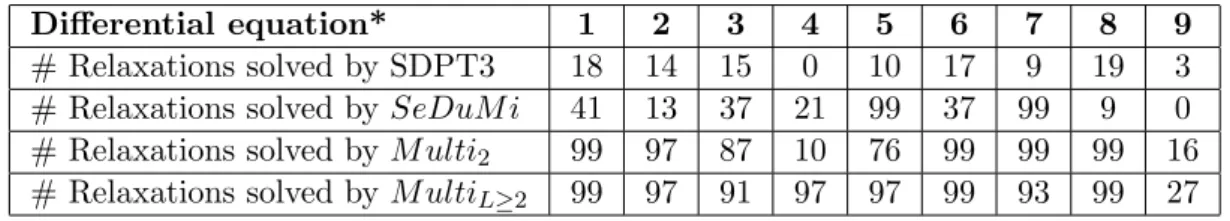
4.5 Comparison between relaxations solved by SDPT3, SeDuMi and the multigrid algorithm as a function of the size of the problem (n) for the non-linear differential equations. . . 110

(9)

LIST OF TABLES

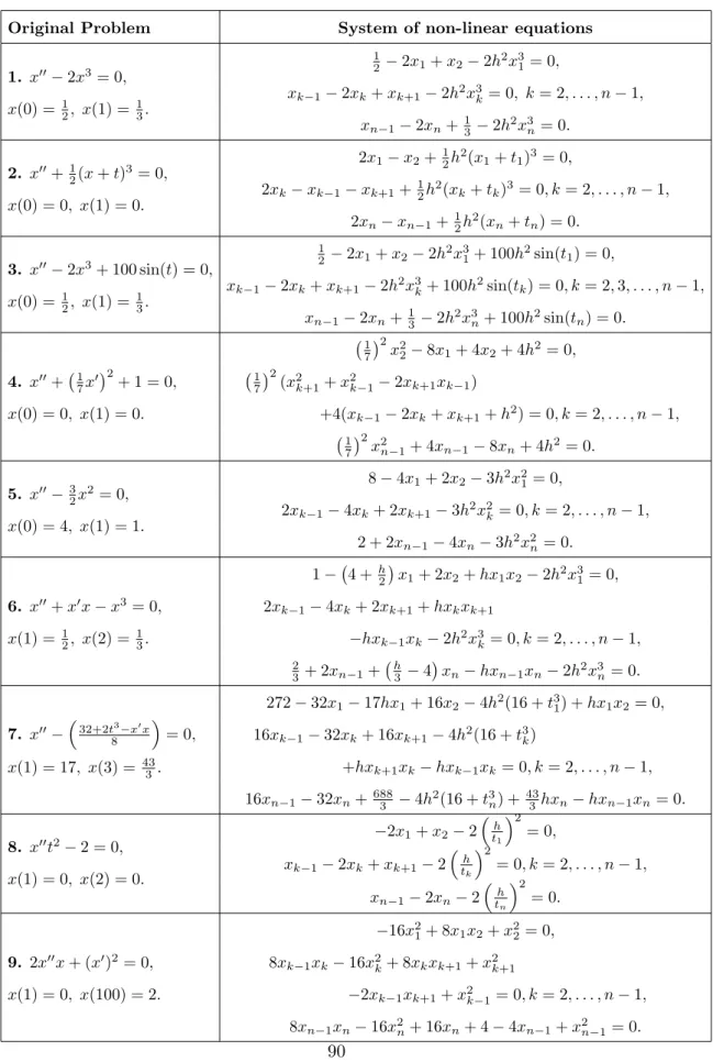
4.1 List of non-linear differential equations. . . 90

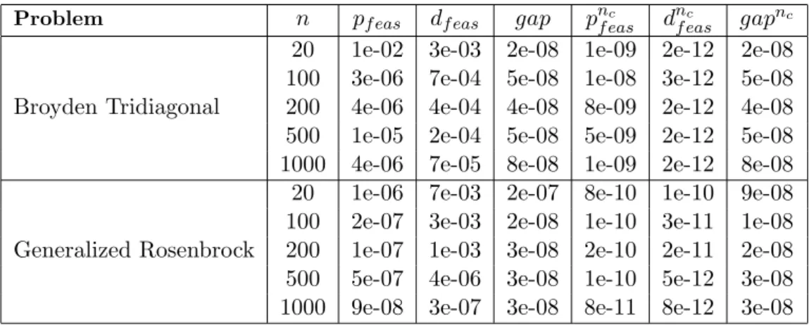
4.2 Feasibility and gaps of projected variables for Broyden Tridiagonal and Generalized Rosenbrock functions. . . 103

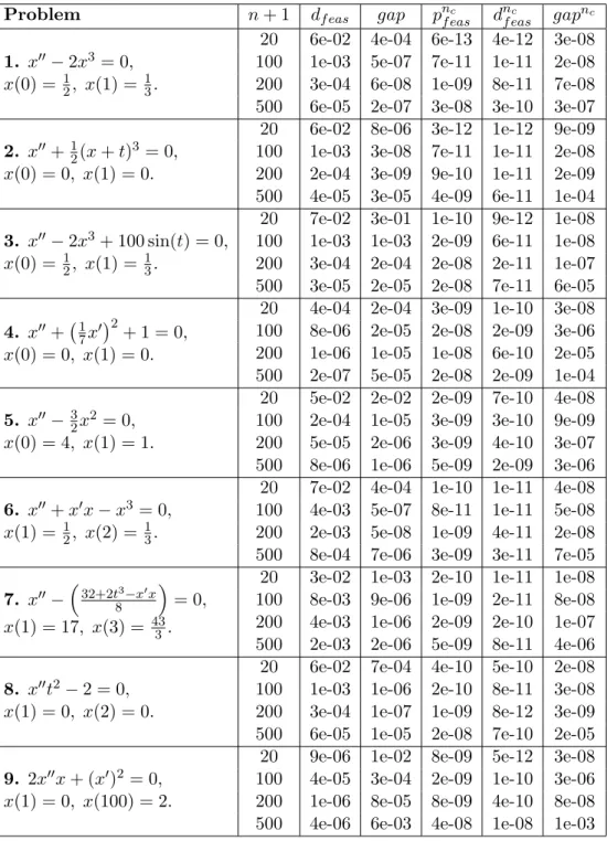
4.3 Feasibility and gaps of projected variables for the non-linear differential equations. . . 104

4.4 Comparison between relaxations solved by SDPT3, SeDuM i and the multigrid approach for the non-linear differential equations. . . 109

4.5 Condition number of the Schur-complement matrix for the last itera-tion at the fine level using SDPT3 and M ultiL≥2 for the non-linear differential equations. . . 111

4.6 CPU time comparison for the non-linear differential equations problems solved to at least a 10−4 accuracy. Small size: n = 20,30, . . . ,100 (9 relaxations per differential equation). . . 113

4.7 CPU time comparison for the non-linear differential equations problems solved to at least a 10−4 accuracy. Medium size: n= 110,120, . . . ,500 (40 relaxations per differential equation). . . 113

4.8 CPU time comparison for the non-linear differential equations problems solved to at least a 10−4 _{accuracy. Large size:} _n _{= 510}_,₅₂₀_{, . . . ,}₁₀₀₀ (50 relaxations per differential equation). . . 114

5.1 Motzkin Polynomial function evaluated at the solution found by the SDP relaxation for different values of M andw.. . . 137

5.2 Number of iterations calculated by SDPT3 to solve the Motzkin Poly-nomial function SDP relaxation for different values of M and w. . . 137

5.3 Duality gap for the wth SDP relaxation of the minimization of the Motzkin function for the prolongated solution of the (w−1)th SDP relaxation. . . 138

(10)

5.4 Motzkin Polynomial function evaluated at the solution found by the SDP relaxation for different values of M and w when the prolongated solution of the (w−1)th SDP relaxation is used as initial point to solve the wth SDP relaxation. . . 139

5.5 Ratio of the time required by SDPT3 and the multilevel approach to solve thewth_{order relaxation for the minimization of the Motzkin}

Poly-nomial (timeSDP T3/timeM ulti). . . 140

5.6 Ratio of the total time required by SDPT3 and the multilevel approach to sequentially solve the SDP relaxations for the minimization of the Motzkin Polynomial until a polynomial solution with an accuracy of 10−7 can be extracted from the SDP relaxation.. . . 141

(11)

LIST OF NOTATION

Vectors and matrices

N: set of non-negative integers;

Rn: n-dimensional real Euclidian vector space; Rm×n: space of real m×n matrices;

[A]i,j =Ai,j : entry (i, j) of A;

Sn={X:X∈_Rn×n, Xi,j =Xj,i} (set of symmetric matrices); Sn

+={X:X∈ Sn, y>Xy≥0 for all y∈Rn}(set of positive semidefinite matrices);

S₊₊n ={X:X∈ Sn, y>Xy >0 for all y∈Rn, y6= 0} (set of positive definite matrices);

X0 :X ∈ S₊n (X is positive semidefinite);

X0 :X ∈ S₊₊n (X is positive definite);

A>: transpose of A∈_Rm×n;

(12)

Tr(A) =X i Ai,i = X i λi(A) (trace of A∈RN×n); hA, Bi= Tr(A>B) (inner product); kAk=phA, Ai (Frobenius norm).

Polynomials Let d ∈_N, Φ ⊆ {1,2, . . . , n}, and let f :Rn 7→ R be a real-valued

polynomial function, such that f(x) = P

α∈_Nnbαxα, where α = [α1, α2, . . . , αn]>, x= [x1, x2, . . . , xn]>,xα=xα11x

α2

2 . . . xαnn, and bα∈Rfor all α∈Nn.

deg(f) = max ( X i αi :α∈Nn, bα6= 0 ) (degree of f); Γn_d ={α∈_Nn:X i αi ≤d};

supp(f) ={α∈Γn_deg(_f₎ :bα6= 0}(support of f);

AΦd ={α∈Nn:

X

i

αi ≤d, αi= 0 if i /∈Φ};

Bi ={α∈Γnd :αi >0, αj = 0 for j < i}, for any 1≤i≤n;

u(x,AΦd) : column vector with monomialsxα forα∈AΦd;

g(k, l) = k+l l = (k+l)! k!l! , for any k, l∈N; α+= [0, α1, α2, . . . , αn−1]> ∈Rn, forα∈Nn; α−= [α2, α3, . . . , αn,0]>∈Rn, forα∈Nn; α−t= [αt+1, αt+2, . . . , αn,0, . . . ,0]>∈Rn, fort∈N, t≥2 and α∈Nn;

(13)

: matrix of dimensions n×n with a non-zero real number in position (i, j) if there existsα∈supp(f) such thatαi >0 and

αj >0, or ifi=j; or zero other wise. CSP graph : correlative sparsity pattern graph;

: graph associated to the CSP matrix. This graph hasn nodes and an edge between node iand j if the CSP matrix has a non-zero element in the (i, j)th entry.

(14)

ONE

INTRODUCTION

During the last few decades Semidefinite Programming (SDP) has been one of the most studied topics in optimization. As mentioned in Todd,2001, there are two main

reasons for its popularity: (a) its capacity to model many problems, and (b) because of the development of efficient algorithms to solve SDPs in polynomial time (specifically Interior Point Methods (IPM)). As it is, several complex and difficult problems in combinatorial optimization, engineering and control theory, among others, have been reformulated or approximated as SDPs. One interesting application for SDPs comes from polynomial optimization problems (POP). In particular, given a POP, Lasserre,

2001creates a hierarchy of SDP relaxations that converge to the solution of the original

POP, thus changing a non-linear and in general non-convex optimization problem, for a convex one. However, when using the classical Lasserre hierarchy, it is only possible to solve problems with a few dimensions due to the size of the resulting SDP relaxations.

(17)

Waki et al., 2006 proposed a sparse version of this hierarchy, where the sparsity of

the polynomial problem is used to reduce the size of the SDP relaxation, allowing to solve POP’s with several hundred variables (Lasserre,2015;Waki et al.,2006). In this

dissertation, we argue that when the SDP approach is used to solve POPs, additional characteristics of the relaxations can be exploited to solve the resulting SDP problems more efficiently.

Our approach is inspired by multigrid methods. When solving a system of linear equations, and in some optimization problems, it is widely accepted that if a multigrid method is applicable, then it is often the best numerical method to use (Borz`ı and

Schulz, 2009; Saad, 2003). For examples of the multigrid approach to various

opti-mization problems we refer the interested reader to Borz`ı and Schulz, 2009; Gratton

et al., 2008; Nash,2000; Wen and Goldfarb, 2009,Hovhannisyan et al., 2016 for

con-vex optimization problems in image processing, and Ho and Parpas,2014for Markov

Decision Processes. The core principle of multigrid methods is to construct a coarse model of the original (high resolution/fine) model and use the information obtained from solving the coarse model to improve the current solution. This approach works extremely well when the coarse and fine model share a common structure. Besides, based on the intuition that the coarse model is a global approximation to the fine model (as opposed to only using local information to construct a search direction) the hope is that multigrid methods can potentially be applied to global optimization problems too. Motivated by the potential numerical improvements and the fact that the coarse model retains global information about the model, we develop the multigrid principle for SDP relaxations of Polynomial Optimization Problems (POP).

(18)

We propose two ideas. The first one comes from the observation that many large scale polynomial optimization problems have their origins from the discretization of an infinite dimensional model. The resulting finite dimensional model is sparse but has a large number of degrees of freedom. Optimization models that fit this class are bound-ary value problems (Papamichail and Adjiman,2002), optimization with PDEs (Hinze

et al.,2008;Borz`ı and Schulz,2011), optimal control (Borz`ı et al.,2002;Dontchev and

Hager,2001), and Markov Decision Processes (Ho and Parpas,2014), among others. In

particular, the problems we study in the first part of this dissertation are unconstrained POPs with a sparse structure, where it is possible to define a hierarchy of POPs by varying the number of variables. A good example of the problems we consider is the Generalized Rosenbrock function: Fn(x) =Pn_k₌₁−1100(xk+1−xk)2+ (1−xk+1)2 (Nash,

1984). This polynomial is sparse in the sense that not all the monomials ofnvariables

have a non-zero coefficient (e.g., x1x2x3x4 does not appear in the function Fn(x)). Note also that by varying the number of variables (n), we can define a family functions that share a similar polynomial structure, say {Fn(x)}n∈Ω for some Ω ⊆ {2,3, . . .}, and that the minimum of each function Fncan be approximated by solving its sparse SDP relaxation (Waki et al.,2006). Another interesting example is the system of

non-linear equations obtained when a finite difference discretization scheme is used to solve polynomial differential equations with boundary conditions (see for example Burden

and Faires,2011); which can be solved by minimizing the sum of the squared errors of

the system of equations (for more details seeChapter 4). As in the Generalized

Rosen-brock case, we can obtain a different system of equations by varying the number of points chosen for the discretization, and use the sparse SDP relaxation to approximate

(19)

their solutions.

A multigrid approach to solve the system of equations withnvariables obtained for the differential equation problem, consists on using the information of a similar lower dimensional problem to solve the high dimensional original one (e.g., use the solution of the system of equations obtained after discretize the domain withn/2 variables to solve the original problem with n variables). Given the efficiency of the multigrid method to solve the n dimensional system of equations, it is interesting to study if a similar approach can be used to solve the SDP relaxations of POPs like the ones mentioned in the previous paragraph (e.g., use the solution of the sparse SDP relaxation of the POP with n/2 variables to solve the sparse SDP relaxation of the POP withn variables).

The first contribution of this thesis is to show how to take advantage of both the sparse and hierarchical structure present in many problems. Our theoretical results suggest that under appropriate conditions we should expect significant improvements in computational complexity. Our numerical results further support this claim, and we show that a multigrid approach can improve the robustness and reduce the time required to solve large scale polynomial optimization problems. In particular, we propose a multigrid framework for the SDP relaxation of the following POP:

min x∈Rn Fn(x), n1−1 X k=1 fk(xk) + n2 X k=n1 f0(xk) + n−p+1 X k=n2+1 fk(xk), (1.1)

wherefk:Rp 7→Rarep-dimensional polynomial functions of degreedk,k= 0,1, . . . , n1− 1, n2+ 1, . . . , n−p+ 1, xk = {xk, xk+1, . . . , xk+p−1} for k = 1,2, . . . , n−p+ 1, and

(20)

problem is sparse in the sense that every variable only appears together withp−1 of its neighbors. In our numerical experiments we typically have n1 = 2 andn2=n−p+ 1. Note, for example, that for the Generalized Rosenbrock function we will have: p= 2,

n1 = 1, n2 = n−1, f0(xk) = 100(xk+1−xk)2+ (1−xk+1)2 for k = 1,2, . . . , n−1,

d0= 4, and fk(xk) = 0 for any k6= 0.

If Problem (1.1) is going to be solved using a sparse SDP relaxation, the main idea

is to define a hierarchy of polynomial problems by reducing the number of variablesn, and use the information of the solution of the SDP relaxation of these reduced order polynomial problems to solve the higher order relaxation. The principal technical diffi-culty of applying multigrid to a (sparse or otherwise) SDP relaxation of Problem (1.1)

is that the information between the variables is lost through the relaxation process. In this thesis, we take the first steps towards addressing this issue. We show that despite the loss of information, it is still possible to obtain useful information from the coarse SDP relaxation and to construct a good approximation to the solution of the fine SDP relaxation. We do not propose a new hierarchy for polynomial problems in the same way thatLasserre,2001did. Instead, we show how the resulting SDP relaxations

pro-posed in Waki et al., 2006, which is the most popular and widely used hierarchy for

sparse problems, can be solved more efficiently by making use of additional structure present in many applications.

We develop this idea inChapter 3 and Chapter 4. In particular, the main

contri-butions of these two chapters are:

(21)

coarse SDP relaxation with the original SDP relaxation for POPs like Problem (1.1). Borrowing terminology from the multigrid literature we call these

opera-tors prolongation operators.

2. Derivation of sufficient, and easily verifiable conditions for these operators to be useful in practice.

3. We show that if our conditions are satisfied, then it is possible to improve the worst case complexity of infeasible interior point methods.

4. Numerical experiments that show that our conditions are indeed satisfied in many practical problems and that our multigrid framework can be used to improve the numerical performance of infeasible interior point methods.

The second idea in this dissertation follows the same multigrid “spirit” but in a different context. More specifically, we no longer assume any particular structure of the underlying polynomial problem, but instead concentrate directly on the hierarchy of relaxations for a fixed POP. As mentioned before, for a given POP a hierarchy of SDP relaxations can be constructed with the property that the solutions of the SDP hierarchy converge to the solution of the POP. One characteristic of this hierarchy, is that the number of variables increases from one level to the next, making it harder to solve higher order relaxations. Then, a natural question is how can we use the information of lower order relaxations to find a solution of higher ones. InChapter 5,

we answer this question by constructing prolongation operators that relate points in the lower (coarse) levels of the hierarchy with the higher (fine) levels. Our main contributions of this chapter are:

(22)

1. The construction of operators that relate the primal and dual solutions of the coarse SDP relaxation with the original SDP relaxation, for any unconstrained polynomial optimization problem

2. We prove that when a coarse optimal point is prolongated using these operators, then the resulting fine point is feasible for the fine relaxation; and furthermore, if the order of the coarse relaxation is high enough in the hierarchy then the prolongated point will be close to optimal for the fine level.

3. We show with an example how these operators behave in practice, and the poten-tial improvement in efficiency that can be obtained when used as starting points along with an interior point method.

A multigrid approach in the context of sparse SDP relaxations was used inMevissen

et al.,2008,2011to solve finite difference approximations to optimal control problem

and PDE problems. However, the authors used the standard multigrid operators to interpolate between the variables in the original space. Whereas, we work directly with the primal/dual variables of the SDP relaxation. The SDP variables contain much more information than just the solution to Problem (1.1). The additional information

can be put to good use in the next level of the hierarchy. This advantage is reflected in our numerical and theoretical results. In particular, we can solve bigger problems with our approach rather than using SDP relaxations as a black box. Another related approach is the application of multigrid methods to SDP relaxations of combinatorial optimization problems (seeLin et al.,2016). Their approach is specific to the particular

(23)

SDP relaxations of Problem (1.1) we consider in this dissertation.

The rest of this dissertation is structured as follows: Chapter 2defines the notation

used, as well as the theoretical background needed for the following chapters. In partic-ular we introduce the reader to the Semidefinite Programming theory and algorithms, and to the use of SDP relaxations to solve POPs. In Chapter 3 we define a lower

dimensional polynomial problems for the POP (1.1), study its SDP relaxations, and

define and analyze prolongation operators for this relaxations. Chapter 4 we report

numerical results for applications of the operators defined in Chapter 3. InChapter 5

we study the hierarchy of SDP relaxations for any unconstrained polynomial optimiza-tion problem, we define prolongaoptimiza-tions operators, analyze them, and illustrate its use with a numerical example. Finally, in Chapter 6 we present conclusions and possible

(24)

CHAPTER

TWO

NOTATION AND BACKGROUND

As mentioned in the previous chapter, this thesis considers sparse SDP relaxations for polynomial optimization problems. In this chapter we describe our notation and provide background material for Semidefinite Programming (SDP) theory and algo-rithms. We also describe the SDP relaxations of polynomial optimization problems that we will use in the rest of the thesis.

2.1 Notation

2.1.1 Matrices

R and N will denote the set of real numbers and non-negative integers respectively.

(25)

denoted byRn(Nnfor non-negative integer entries). Ifxis a column vector then itsith

component will be denoted byxi (if the name of the vector includes a subscript and/or a superscript we will use [x]i). Likewise, if m, n ∈ N are two positive integers, then Rm×n is the set of matrices withm rows and n columns. For any matrixA ∈Rm×n,

Ai,j will correspond to the element in position (i, j) (if the name of the matrix includes a subscript and/or a superscript we will use [A]i,j). The superscript “>” on top of any matrix will denote the transpose of the matrix. For anyA∈_Rn×n_{, the trace operator} is defined as Tr(A) , Pn

i=1Ai,i. If A, B ∈ Rm

×n _{are two matrices we will use the}

Frobenius inner product which is defined as

hA, Bi_,Tr(A>B) = m X i=1 n X j=1 Ai,jBi,j,

and its induced norm

kAk_,phA, Ai=

s X

i,j

(Ai,j)2.

If A is a one dimensional matrix (i.e., a real number), its norm is just the absolute value and in this case we will use the standard notation |A|. If A ∈ _Rn×n_{, the} _kth order leading principal sub-matrix of A is the square matrix obtained after deleting the lastn−k rows and columns of A.

The set ofn×nsymmetric matrices will be represented by Sn _{. For any} _A_{∈ S}n_, if x>Ax ≥ 0 (x>Ax > 0) for any non-zero x ∈ _Rn_{, then} _A _{is said to be positive} semidefinite (positive definite). If A is positive semidefinite it will be denoted by

(26)

definite) matrices bySn

+(S++n ). Although in some books a positive semidefinite matrix is not necessarily symmetric, in this work if a matrix is positive semidefinite (or positive definite), it will be assumed to be symmetric. IfA∈ Sn_{, then}_λ

i(A) will represent the

ith eigenvalue of A where λ1(A) ≤λ2(A) ≤ · · · ≤λn(A). The identity matrix will be denoted by I ∈_Rn×n _{and its size will be understood from the context.}

For any set Ω,|Ω|is the cardinality of the set, and its kth-Cartesian product will be the set {Ω}k ₌ _{₍_v

1, v2, . . . , vk) : vi ∈Ω fori = 1,2, . . . , k}. Finally, if A⊆B are two sets, B\A={x:x∈B, x /∈A}.

2.1.2 Polynomials

Letx= [x1, x2, . . . , xn]∈Rn andα= [α1, α2, . . . , αn]∈Nn be twondimensional

vec-tors, and f :Rn→Ra real-valued polynomial function. The monomialxα11x

α2

2 . . . xαnn will be denoted by xα, and its coefficient in the function f as bα ∈ R. The degree

of the polynomial f is defined as deg(f) , max{P

iαi :α∈Nn, bα6= 0}. Letting

Γn_d , {α ∈ _Nn _: P

iαi ≤ d}, any polynomial of degree at most d can be writ-ten as f(x) = P

α∈Γn dbαx

α_{. The support of a polynomial function} _f _{of degree} _d

is defined by supp(f) , {α ∈ Γn_d : bα 6= 0}. For any set Φ ⊆ {1,2, . . . , n}, let

AΦd = {α ∈ Nn :

P

iαi ≤ d, αi = 0 ifi /∈ Φ} and u x,AΦd

be a column vec-tor with the monomials xα _for _α _∈

AΦd. For example if Φ = {2,4} and d = 2,

u x,AΦd

= [1, x2, x4, x22, x2x4, x24]>. The size of the vector u x,AΦd

is equal to

|Φ|+d d

= (|Φ_|_Φ|_|+_!_dd_!)!, and will be denoted by g(|Φ|, d), where |Φ| corresponds to the number of elements in the set Φ. Without loss of generality, throughout this entire dissertation it will be assumed that for any Φ ⊆ {1,2, . . . , n} the vector u x,AΦd

(27)

sorted in ascending order according to a fixed monomial ordering (seeCox et al.,1992

for information on monomial orderings).

This notation is standard in the polynomial literature and we refer the reader to

Waki et al.,2006for more details. Below we introduce two definitions that are specific

to this work.

Definition 2.1. For any 1≤i≤n let Bi ,{α∈Γn_d :αi>0, αj = 0 for j < i}.

Remark 2.1. Note thatΓn_d\ {0}=∪n

i=1Bi, andBi∩Bj =∅ for anyi6=j. Example 2.1. If n=d= 2 then:

Γn_d ={[0,0]>,[1,0]>,[0,1]>,[2,0]>,[1,1]>,[0,2]>}, B1 ={[1,0]>,[1,1]>,[2,0]>},

B2 ={[0,1]>,[0,2]>}.

Definition 2.2. If α∈_Rn _{is equal to}_[_α

1, α2, . . . , αn]>, thenα+,α−∈Rnare defined

as α+ ,[0, α1, α2, . . . , αn−1]> and α− ,[α2, α3, . . . , αn,0]>. Likewise, if t ∈N and

t≥2, then α−t∈_Rn _{is defined as} _α−t_,_[_α

t+1, αt+2, . . . , αn,0, . . . ,0]>.

Example 2.2. Let α = [1,4,6,0]>. Then α− = [4,6,0,0]>, α+ _{= [0}_,₁_,₄_,_6]> _and α−2= [6,0,0,0]>.

Remark 2.2. Let Φi = {i, i+ 1, . . . , i+p−1}, for some i, p ∈ N. Note that under

the assumption of the ordering of the vectors u x,AΦd

,if xαis the kth element in the vector ux,AΦ_di

thenxα+ _{is the} _kth _{element in the vector} _u_x_,

AΦ_di+1

. Similarly if

xα is the kth element in the vector ux,AΦdi+1

(28)

vector u

x,AΦdi

.

Example 2.3. Consider the following ordering for the vector u x,AΦd

where Φ ⊆ {1,2, . . . , n}: u x,AΦd = [1, xi1, xi2, . . . , xim, x 2 i1, xi1xi2, . . . , xi1xim, x 2 i2, . . . , x 2 im, . . . , x d i1, . . . , x d im] >_,

where m=|Φl|, and i1 < i2 <· · ·< im. Letting Φ2 ={2,3}, Φ3 ={3,4} and d= 2,

we haveux,AΦ2_d = [1, x2, x3, x22, x2x3, x23]>andu x,AΦ3_d = [1, x3, x4, x23, x3x4, x24]>.

Note for example that ifα= [0,1,1,0]thenα+ = [0,0,1,1], and both, xα=x2x3 and xα+ =x3x4, are the fifth element ofu

x,AΦ2_d and u x,AΦ3_d respectively.

2.2 Background

2.2.1 Semidefinite Programming and Interior Point Methods

This section contains the basic properties of Semidefinite Programming (SDP) that will be needed later on. We also include a brief discussion on Interior Point Methods (IPM). We follow closely the work inTodd,2001;de Klerk,2002;Alizadeh et al.,1998.

Let C, Ai ∈ Sn for i= 1,2. . . , m, b ∈ Rm, and assume without loss of generality

that the matrices {Ai}mi=1 are linearly independent. For this document, the primal SDP problem is:

(29)

min y,S b >_y s.t. m X i=1 Aiyi+C=S, S0. (2.1)

The dual of this problem is

max

X − hX, Ci

s.t. hAi, Xi=bi, i= 1,2, . . . , m,

X 0.

(2.2)

It is important to note that this presentation of the SDP problem is slightly different from the standard primal and dual SDPs definition presented in the literature, where Problem (2.1) is known as the dual problem and Problem (2.2) as the primal. We

make this change to be consistent with the exposition of the SDP relaxations. It is possible to deduce that both the standard definition and Problems (2.1) and (2.2) are

equivalent.

LetA:Rn×n−→Rm be the linear operator defined as

A(X),[hA1, Xi,hA2, Xi, . . . ,hAm, Xi]>.

Let A>_:

(30)

Using these we can rewrite Problem (2.1) as min y,S b >_y s.t. A>(y) +C=S, S 0, (2.3) and Problem (2.2) as max X − hC, Xi s.t. A(X) =b, X 0. (2.4)

Hence, a semidefinite program is a minimization of an affine function with affine constraints where the variable is a square matrix which has to be positive semidefinite. Given that the set of positive semidefinite matrices is a convex cone, we have that both problems (2.1) and (2.2) are convex problems. As in linear programming, weak

duality is satisfied.

Lemma 2.1. If (y, S) and X are feasible for problems (2.1) and (2.2) respectively, then

b>y−(− hC, Xi) =hX, SiTr(XS)≥0.

Proof. See Proposition 2.1. inTodd,2001.

However, if (X?, y?, S?) are optimal solutions to problems (2.3) and (2.4), it is

not true in general that Tr(X∗S∗) = 0 (the zero duality gap property does not hold for every SDP). This important property can be achieved under certain qualification

(31)

constraints for SDPs. Letp? _and _d? _{be the optimal values of problems (}_2.3_{) and (}_2.4₎

respectively, and define the sets P , {(y, S) ∈ _Rm_{× S}n _: _A>₍_y_{) +}_C ₌ _{S, S} ₀_}_, P? , {(y, S) ∈ P :b>y = p?}, D , {X ∈ Sn _: _A₍_X_{) =} _{b, X} ₀_} _and _D? _, _{_X _∈

D :− hC, Xi =d?}. If there exists (y, S) ∈P such that S 0 we will say that P is strictly feasible, conversely, if there existsX ∈D such thatX 0 we will say that D

is strictly feasible.

Theorem 2.1. If P is strictly feasible and p?>−∞, then p? =d?,P? 6=∅ and there exists X ∈D such that X0. Conversely, if D is strictly feasible and d? <∞, then p?=d?, D? 6=∅ and there exists(y, S)∈P such that S 0.

Proof. See Theorem 2.2. inde Klerk,2002.

Thus, if we assume the existence of strictly feasible primal and dual points (Slater’s constraint qualification), the strong duality holds as long as the optimal values of problems (2.1) and (2.2) are bounded. In this case necessary and sufficient optimality

conditions for the primal and the dual problems are given by:

A>(y) +C =S, S0,

A(X) =b, X 0, XS = 0.

(2.5)

Note that the last equality in Problem (2.5) is equivalent to the duality gap being

(32)

Interior Point Methods

Interior Point Methods (IPM) are the most popular algorithms for SDPs. There are several variants of the IPM framework. We will discuss primal - dual path following methods and refer the reader tode Klerk,2002;Todd,2001;Wolkowicz et al.,2012for

a deeper and more comprehensive study of the topic.

Primal - dual methods use a perturbed version of the optimality conditions (2.5),

transforming the last equality fromXS= 0 toXS =µI, withµ >0 andIthe identity matrix. Of course, if µ is equal to zero we have the original system (2.5). The new

system of equations is then

A>(y) +C =S, S0,

A(X) =b, X 0, XS =µI.

(2.6)

Theorem 2.2. For everyµ >0, if P andD are strictly feasible, then the system (2.6)

has a unique solution.

Proof. See Theorem 5.2. inTodd,2001.

Forµ >0 let (y?

µ, Sµ?, Xµ?) be the solution of the system (2.6). The set of solutions of the system (2.6) for allµ >0 is called the central path. DefineCP ,{(y?_µ, S?_µ, X_µ?) :

µ >0} as the central path.

Theorem 2.3. If P and Dare strictly feasible, the setCP forms a non-empty differ-entiable path. Furthermore, any point (y_µ?, S_µ?, X_µ?) ∈ CP is strictly feasible, and the

(33)

duality gap is given by

b>y?_µ−(−

C, X_µ?) = Tr(X_µ?S_µ?) =nµ.

Proof. See Theorem 5.3. and 5.4. inTodd,2001.

Therefore, starting with some µ0 > 0 and points (y, S, X) such that X 0 and

S 0, the basic idea is to follow the central path generating a sequence of solutions {(y?_µ_i, S_µ?_i, X_µ?_i)}k

i=0 of the system (2.6), with 0 < µk < µk−1 < ... < µ0 for some µk small enough such that Tr(X_µ?_kS_µ?_k) < , for some >0. However, solving the system (2.6) for a given µ can be expensive and unnecessary. Therefore, the usual strategy

consists of generating a sequence that belongs to a neighborhood of the central path.

Given a point (y, S, X), the system (2.6) is used to generate a direction (∆y,∆S,∆X)

by solving,

A>(∆y)−∆S=S−C− A>(y),

A(∆X) =b− A(X),

(X+ ∆X)(S+ ∆S) =µI.

(2.7)

Note that although the direction ∆S will be symmetric if S is symmetric (the first equation will enforce that condition), the same can not be guaranteed for ∆X. There-fore a symmetrization scheme is necessary. Several approaches have been proposed to obtain a symmetric solution for X. For example, in Alizadeh et al., 1998 the

last equation of the system (2.6) is replaced for 1₂(XS +SX) = µI. Other,

popu-lar approaches include the directions proposed by Kojima et al., 1997; Nesterov and

(34)

examples of the family of directions (known as the MZ directions) obtained by re-placing the last equation of the system (2.6) for HP(XS) = µI, where HP(M) =

0.5[P M P−1+ (P M P−1)>] for a given non-singular matrix P (Zhang,1998). In this

case, depending of the choice of P, different directions can be formed. For example, ifP =I orP =X1/2(X1/2SX1/2)−1/2X1/2, the directions inAlizadeh et al.,1998or

Nesterov and Todd, 1997would be obtained respectively. A generic primal-dual path

following IPM is described in Algorithm 1, where HP(XS) = µI is used to replace

XS =µI for a suitable matrix P.

Algorithm 1 Generic primal-dual path following Interior Point Method. Input: X0 ∈ Sn

++, S0 ∈ S++n , y0∈Rm, 0≤σ <1, tolerance level >0. Procedure:

- Set r = max{Tr(X0S0),kA(X0)−bk,kA>(y0) +C −S0k}, µ0 = σTr(X_n0S0) and

k= 0.

whiler > do

- Calculate directions (∆y,∆S,∆X) by solving the system A>(∆y)−∆S=Sk−C− A>(yk),

A(∆X) =b− A(Xk),

HP(∆XSk+Xk∆S) =µkI−HP(XkSk). - Choose step-lengths a1 and a2 and set

yk+1 =yk+a1∆y, Sk+1=Sk+a1∆S, Xk+1 =Xk+a2∆X. - Set r = max{Tr(Xk+1Sk+1),kA(Xk+1)−bk,kA>₍_yk+1_{) +}_C₋_Sk+1_k}_,_µk+1 ₌ σTr(Xk+1_nSk+1) and k=k+ 1. end while

The strategy to select the step-lengthsa1 anda2 must guarantee that at iteration

kthe matricesSk+a1∆S andXk+a2∆Xare positive definite, and also that the new iterate (yk+1, Sk+1, Xk+1) belongs to a neighborhood of the central path (for more on

(35)

the selection of the step-lengths and the value σ see Alizadeh et al., 1998). Solving

the system of linear equations to find the directions (∆y,∆S,∆X) at iteration k, can be reduced by block Gauss elimination to solving a linear system Mk∆y = dk,

where the matrices Mk ∈ _Rm×m _and _dk _∈

Rm depend on (yk, Sk, Xk), µk and P

(i.e., the symmetrization scheme adopted). The matrix Mk is known as the Schur

complement matrix, and the majority of the computing time is spent on forming this matrix and solving the system for the variable ∆y. In practice, the stability of the algorithm depends on this matrix, and therefore characteristics like a low condition number are desirable. See Alizadeh et al.,1998;Todd et al.,1998 for analysis on the

Schur complement matrix.

The previous algorithm is an infeasible IPM because the sequence{(yk, Sk, Xk)}_k is not necessarily feasible (although Sk, Xk are positive definite). Other versions of IPMs include feasible IPMs, where for any k the sequence (yk, Sk, Xk) is feasible (see for exampleMonteiro,1997), as well as the predictor-corrector algorithm ofTodd et al.,

1998and self-dual embedding strategies (de Klerk et al.,1997).

Polynomial complexity has been proved for IPMs. For example, in Potra and

Sheng, 1998 an infeasible algorithm is proposed, and it is proved that if the initial

point is feasible (or close to feasible), then it will require no more thanO(√nln(0/)) iterations to find a solution with tolerance , where0 is a measure of the error of the initial point. For feasible algorithms polynomial results can be found for example in

Monteiro,1998, where it is proved that ifL >1 thenO(√nL) iterations are needed to

reduce the duality gap by a factor at least 2−O(L) for an IPM based on the MZ family of directions.

(36)

Other approaches for large scale SDP

IPMs are the most efficient algorithms to solve small to medium size semidefinite programming problems. In fact, it has been observed that independent of the size of the problem, the number of iterations needed to solve a SDP does not change much, and it is lower than the predicted worst case scenario complexity (Boyd and Vandenberghe,

1996). Their efficiency depends strongly on the work done at each iteration to calculate

the search directions. For example, if the number of constraints of the problem is m, then at each iteration it is necessary to construct anm×mmatrix (Schur complement matrix). If Cholesky factorization is used to solve the system of linear equations, the total work for one iteration in terms of arithmetical operations isO(m3) and hasO(m2) storage requirements. Therefore, the use of IPM becomes intractable both in terms of time and memory when the problem is large.

As alternatives for large SDPs, first order algorithms have been developed. We describe two methods that have been very efficient for large SDPs.

Alternating Direction Method of Multipliers

One of the most successful frameworks for large scale problems is the use of the method of multipliers for the primal problem (2.1) (Bertsekas, 2014). The boundary point

method introduced by Povh et al., 2006, as well as the alternating direction of Wen

et al., 2010, construct an algorithm based on this method (although the boundary

method described in Povh et al.,2006 differs in some aspects from Wen et al.,2010,

(37)

central idea is to repeat the following two operations until a stopping condition is reached: minimize the augmented Lagrangian for the primal variables keeping con-stant the Lagrangian variable and then, using the new primal variables, update the Lagrangian variable according to a fixed rule. One important feature of these algo-rithms that differentiate them from IPMs is that the sequence of points generated are such that they do not lie in the interior of the positive semidefinite cone but on the boundary. They also satisfy the third equation of the optimality conditions (2.5) at

every iteration (the non-optimality comes from the violation of the first two equations). Therefore, instead of reducing the duality gap the algorithm is trying to reduce the infeasibility with respect to the linear constraints of the primal and the dual.

IfLa

σ(y, S, X) =b>y+

X,−A>₍_y_{) +}_S₋_C

+₂1_σk − A>₍_y_{) +}_S₋_C_k2 _for_{σ >}_0,

Algorithm 2 describes the methodology.

Algorithm 2 Alternating Direction Method of Multipliers. Input: X0 = 0,S0 = 0, σ >0, tolerance level >0. Procedure:

- Setk= 0 and r= max

n_kA (Xk₎₋_b_k 1+kbk , kA>₍_yk₎₊_C₋_Sk_k 1+kCk o . whiler < do - Set yk+1 = arg min_y∈_RmLa_σ(y, Sk, Xk). - Set Sk+1= arg min_S∈Sn +L a σ(yk+1, S, Xk). - Set Xk+1 =Xk+−A >₍_yk+1_{) +}_Sk+1₋_C σ .

- Setr = maxnkA(X₁₊k_k+1_b_k)−bk,kA>(yk+1₁₊)+_k_CC_k−Sk+1ko, and k=k+ 1. end while

(38)

mini-mized, and then use that solution to update the Lagrangian variables. But note that solving the augmented Lagrangian for y fixing S and then for S fixing y, no longer minimizes the Lagrangian with respect to both dual variables. However, the minimiza-tion problems using this approach are easy to solve: the problem for y is equivalent to a linear system of equations, while the problem for S is equivalent to an eigenvalue decomposition of a matrix. It can be shown that this algorithm converges for any value of σ, and therefore the penalty parameter does not change like in the other aug-mented Lagrangian methods (although in practical applications the parameter changes for every iteration to obtain faster convergence).

(Majorized) Newton CG augmented Lagrangian

In the same spirit of Povh et al., 2006; Wen et al., 2010, an inexact augmented

La-grangian method is used in Zhao et al., 2010 (see Rockafellar, 1976a,b for more

in-formation on augmented Lagrangian methods). In this case, if Q Sn

+(Z) is the pro-jection of Z ∈ _Rn×n _{over the positive semidefinite cone} _Sn

+, and σ > 0, the aug-mented Lagrangian for the primal problem (2.1) is defined as La

σ(y, X) = b>y + 1 2σ kQ Sn +(−X+σ(A

>₍_y_{) +}_C₎_k2_{− k}_X_k2_{. This function differs from the one}

pro-posed inWen et al.,2010, because it replaces the semidefinite constraint for the primal

variable using the projection operator to replace the matrix primal variable S.

The Newton CG Augmented Lagrangian is presented inAlgorithm 3. In this case,

the augmented Lagrangian for a givenX is minimized for the primal variabley. How-ever, although this problem is convex, it is not twice continuously differentiable. To solve this problem a conjugate gradient method combined with a semismooth Newton

(39)

algorithm is used. The non-optimality at every iteration comes from the dual and primal infeasibility of the equality constraints (like in the Alternating Direction Aug-mented Lagrangian method). Yang et al., 2015 improves this algorithm by replacing

the semismooth Newton method by a majorized semismooth Newton method, which can handle degenerate SDPs better.

Algorithm 3 (Majorized) Newton CG Augmented Lagrangian. Input: X0 ∈Sn,y0∈_Rm_,_σ0 _>_0,_{ρ >}_{1 tolerance level}_>_0. Procedure: - Set k = 0, W = Xk −σk A>(yk) +C, Sk = Q Sn +(W)−W /σk, and r = max n_kA (Xk₎₋_b_k 1+kbk , kA>₍_yk₎₊_C₋_Sk_k 1+kCk o . whiler < do - Set yk+1≈arg min y∈_RmL a σk(y, Xk). - Set Xk+1=Y Sn + (Xk−σk A>(yk+1) +C . - SetW =Xk+1−σk(A>(yk+1) +C) and Sk+1= Q Sn +(W)−W σk .

- Set r = maxnkA(X₁₊k_k+1_b_k)−bk,kA>(yk+1₁₊)+_k_CC_k−Sk+1ko,σk+1 ₌_ρσk _or_σk+1 ₌_σk_{, and}

k=k+ 1. end while

Other approaches to solve large scale SDPs include Low Rank algorithms (Burer

and Monteiro,2003;Burer and Choi,2006), Proximal methods (Lan et al.,2011), the

row by row method ofWen et al.,2009, and first order block-decomposition ofMonteiro

et al.,2014. Finding a good initial solution with the Alternating Direction Multipliers

Method, and then using this solution as initial point for the Majorized semismooth CG method, was shown to be very efficient in practice (see the numerical results in

(40)

Yang et al., 2015).

2.2.2 SDP relaxations for unconstrained Polynomial Optimization

Problems (POPs)

Let f :Rn 7→ R be a polynomial function of degree 2d. Write f(x) = Pα∈Γn

2dbαx

α

and consider the global unconstrained polynomial optimization problem

min x∈Rn X α∈Γn 2d bαxα. (2.8)

The POP (2.8) can be non-linear and non-convex, and therefore finding a global

minimum is in general a hard problem (see Nesterov, 2000 and Murty and Kabadi,

1987for some examples of NP-hard and co-NP-complete unconstrained POPs).

2.2.3 Dense (Lasserre) relaxation

Lasserre,2001developed a hierarchy of SDP relaxations for polynomial minimization

known as the Lasserre Hierarchy, and proved that under certain assumptions it is possible to extract an approximate solution for problems like Problem (2.8) from the

solution of these relaxations (Henrion and Lasserre,2005). Iff?_{is the global minimum}

of Problem (2.8), then this hierarchy can be obtained by viewing Problem (2.8) as

a moment problem or trying to compute a sum-of-squares decomposition of f(x)−

f? (Parrilo, 2003; Parrilo and Sturmfels, 2003). It is important to note that the

Lasserre Hierarchy also includes the case for constrained POP, but we concentrate on the unconstrained case as is the one used in this dissertation.

(41)

To formulate the hierarchy we first need to define the concepts of moment and localizing matrices. Let w be a positive integer, and y = {yα}α∈Γn

2w a sequence of

real variables indexed by the set Γn₂_w withy[0,0,...,0]= 1. Then, Mw(y) is a symmetric matrix such that if the entriesithandjthof the vectorux,A{w1,2,...,n}

arexαandxβ respectively, then the entry (i, j) ofMw(y) is equal toyα+β. The matrixMw(y) is called the wth moment matrix. Similarly, given a polynomial function θ(x) =P

γ∈Nnθγx α_,

the localizing matrix Mw(θy) is the matrix such that if xα and xβ are the ith and

jth elements of the vectoru

x,A{w1,2,...,n}

, then the entry (i, j) ofMw(θy) is equal to

P

γ∈supp(θ)θγy{γ+α+β}.

Example 2.4. Let n = 2 and θ(x) = 3−2x2₂. Then, u x,A{11,2} = [1, x1, x2]>, ux,A{21,2}

= [1, x1, x2, x21, x1x2, x22]>, and the moment and localizing matricesM1(y),

M2(y) and M1(θy) are

M1(y) =         1 y[1,0] y[0,1] y[1,0] y[2,0] y[1,1] y_[0_,_1] y_[1_,_1] y_[0_,_2]         , M2(y) =                      1 y[1,0] y[0,1] y[2,0] y[1,1] y[0,2] y[1,0] y[2,0] y[1,1] y[3,0] y[2,1] y[1,2] y_[0_,_1] y_[1_,_1] y_[0_,_2] y_[2_,_1] y_[1_,_2] y_[0_,_3] y[2,0] y[3,0] y[2,1] y[4,0] y[3,1] y[2,2] y[1,1] y[2,1] y[1,2] y[3,1] y[2,2] y[1,3] y_[0_,_2] y_[1_,_2] y_[0_,_3] y_[2_,_2] y_[1_,_3] y_[0_,_4]                      ,

(42)

M1(θy) =         3−2y_[0_,_2] 3y_[1_,_0]−2y_[1_,_2] 3y_[0_,_1]−2y_[0_,_3] 3y[1,0]−2y[1,2] 3y[2,0]−2y[2,2] 3y[1,1]−2y[1,3] 3y[0,1]−2y[0,3] 3y[1,1]−2y[1,3] 3y[0,2]−2y[0,4]         .

Note that the 3 principal sub-matrix of M2(y) is exactly the matrix M1(y) (a pattern

present when the vectoru x,AΦ_d is ordered as in this example andExample 2.3). This

fact is also true for the moment localizing matrix with this ordering (i.e., the 3 principal sub-matrix ofM2(θy)is exactly the matrixM1(θy)). Finally, also note that the moment

matrixM2d(θy)can be calculated by replacing the monomials xαfor the variable yαin

the equation u x,AΦd

u x,AΦd

>

. For example, note that ux,A{11,2}

ux,A{11,2} > can be written as u x,A{11,2} u x,A{11,2} > = [1, x1, x2]>[1, x1, x2] =         1 x1 x2 x1 x21 x1x2 x2 x1x2 x22         .

Note thatM1(y) can be constructed by using the previous matrix and replacing xα11x

α2 2

by y_[_α₁_,α_2]. Likewise, the localizing matrix M2d(θy) can be calculated by replacing the

monomials xα for the variable yα in the equation u x,AΦd

u x,AΦd

> θ(x).

(43)

min y X α∈Γn 2w bαyα s.t. Mw(y)0, Mw−1(θy)0, (2.9)

where θ(x) =a2− kxk2 _{for some}_{a >}_{0. Problem (}_2.9_{) defines an infinite hierarchy of}

SDP relaxations indexed by the parameter w. Note that when w > d ifα ∈Γn₂_w and

P

iαi>2d, then bα is equal to 0.

The next theorem shows that by solving the SDP relaxation one can approximate to any required accuracy the optimal global minimum of the unconstrained POP. Moreover, algorithms explaining how to extract an approximate solution x from the SDP solution can be found in Henrion and Lasserre,2005.

Theorem 2.4. Letf?be the global minimum of the POP (2.8), and assume there exists

x? such that kx?k ≤a for some a >0 and f(x?) =f?. If f_SDP? _w is the minimum of the SDP relaxation (2.9), then

(a) As w → ∞ one has f_SDP?

w → f

?_{. Furthermore, for} _w _{sufficiently large there is}

no duality gap for the SDP relaxation (2.9), and its dual is solvable.

(b) f_SDP? w = f ? _{if and only if} _f_(x) ₋_f? ₌ Pr1 i=1qi(x)2 +θ(x) Pr2 j=1tj(x)2, for

some polynomials qi (i= 1,2, . . . , r1) of degree at mostw, and some polynomials

tj(x) (j = 1,2, . . . , r2) of degree at most w−1. In this case, the vector y? ,

{(x?)α}α∈Γn

2w is a solution of the SDP relaxation (2.9).

(c) If f(x)−f? is a sum of squares polynomials (i.e., it can be written asP qi(x)2

(44)

setting θ(x) = 0 in Problem (2.9), and denote its minimum byf?

SDPSOS . Then

for any w ≥ d, f_SDP?

SOS = f

?_{, and the vector} _y? _, _{_xα_} α∈Γn

2w is a solution of

the new SDP relaxation for any x such thatf(x) =f?.

Proof. See Theorem 3.2. and 3.4. inLasserre,2001.

2.2.4 Sparse relaxation

Note that the size of the moment and localizing matrices, as well of the size of y in the SDP relaxation (2.9), depend on the orderw and the number of variables n. For

example, Mw(y) is a square matrix of dimension g(n, w) = n+_ww

= (n_n+_!_ww_!)!, and y a vector of dimension g(n,2w). Then if n = 100 and w = 2, the SDP relaxation will have matrices with dimension larger than 5000 and more than 4 million variables (and therefore more than 4 million constraints in its dual problem). This means that the Lasserre Hierarchy is limited to POPs with objective functions with small number of variables and/or degree. If the number of elements in the support is small, Waki

et al.,2006 developed a sparse SDP relaxation that reduces the number of variables

and constraints compared with the Lasserre SDP relaxation. In order to define the sparse hierarchy it is necessary to define some concepts of Graph Theory.

An undirected graphG(V, E) consists of a setV of nodes and a set of bidirectional edges E, such that ifu, v∈V are connected in the graph then{u, v} ∈E. Two nodes

u, v∈V are said to be adjacent if {u, v} ∈E. A graphGis said to be complete if all the nodes in V are pairwise adjacent (i.e., for any u, v ∈ V {u, v} ∈ E). If W ⊆ V, the sub-graph ofGinduced by W is the graphG(W, E(W)) whereE(W) ={{u, v} ∈

(45)

E : u, v ∈ W}. A clique of the graph G(V, E) is a subset W ⊆ V such that the sub-graph of G(W, E(W)) induced byW is complete. A clique W is maximal ifW is not contained in any other clique. A simple path of length kfromv0 tovkof G(V, E), is a sequence of nodes {v0, v1, v2, . . . , vk} such that vi ∈V (i= 0,1,2, . . . , k), vi 6=vj if i6=j and {vi, vi+1} ∈ E for 0≤i≤k−1. If in additionv0 =vk, the simple path is called a simple cycle of length k+ 1 in G(V, E). Let{v0, v1, v2, . . . , vk} be a simple path ofG, then a chord is an edge between two non-consecutive nodes in the path (i.e., {vi, vj} is a chord if {vi, vj} ∈E and |i−j| ≥2). G(V, E) is a chordal graph if every cycle greater than 3 has a chord. The graph G(V, E0) is called a chordal extension of

G(V, E) ifE ⊆E0andG(V, E0) is chordal. The minimum chordal extension ofG(V, E) is the chordal extension with the least number of edges. Let G(V, E) be a graph with

n nodes, then G(V, E) is said to be an interval graph if there existn intervals in the real line, Ai = [ai, bi] fori= 1,2, . . . , n, such that ifAi∩Aj 6=∅ then{vi, vj} ∈E.

The sparse relaxation for Problem (2.8) proposed in Waki et al., 2006 used the

structure of the so called correlative sparsity pattern matrix (CSP matrix). The CSP matrix for a polynomial is defined as follows,

Ri,j =                      ? ifi=j,

? ifαi ≥1 and αj ≥1 for someα∈supp(f),

0 otherwise,

(2.10)

where?is a non-zero scalar. This matrix has a non-zero element in the component (i, j) if there exists a monomial with variables xi and xj which has a non-zero coefficient

(46)

in the objective function f (i.e., if there exists α ∈ supp(f) such that αi > 0 and

αj >0). IfRis sparse, then Problem (2.8) is called correlatively sparse. Associated to

the CSP matrix is the correlative sparsity pattern graph (CSP graph) G(V, E). The node set is V = {1,2, . . . , n} and E = {{i, j} : i, j ∈ V, Ri,j = ?, i < j}. The idea is to generate a set of supports sets for the polynomial function using the maximal cliques of this graph. However, finding the maximal cliques of a graph is in general NP-hard (see for exampleBomze et al.,1999). In contrast, finding the maximal cliques

of a chordal graph can be done efficiently (Blair and Peyton, 1993; Golumbic, 2004)

and for this reason the sparse relaxations are defined using the maximal cliques of a chordal extension of the CSP graph. Although any chordal extension is valid, the extension with the least number of added edges, a problem known to be NP-complete (Yannakakis,1981), will reduce the size of the final sparse SDP relaxation. In practice,

Waki et al.,2006calculate the minimum chordal extension with heuristics.

Let Φl (l = 1,2, . . . , m) be the maximal cliques of a chordal extension ofG(V, E) and note that M ,zz> is a positive semidefinite matrix for any real vectorz. There-fore, we can add the constraintsu x,AΦl

w u x,AΦl w > 0 (l= 1,2, . . . , m) to Problem (2.8) and obtain the following equivalent problem,

min x∈_Rn X α∈Γn 2d bαxα s.t. u x,AΦwl u x,AΦwl > 0, l= 1,2, . . . , m, (2.11)

where w ≥ d is a degree that denotes the relaxation order. Note that the left hand side of constraint l is a square matrix containing monomials xα for α ∈ _AΦl

2w. Let MΦl w (xα) =u x,AΦwl u x,AΦl w >

(47)

the real variable yα, thewth sparse SDP relaxation is given by min y X α∈F bαyα s.t. MΦl w (y)0, l= 1,2, . . . , m, (2.12) where F =∪m l=1A Φl

2w \ {0}. The matrix MwΦl(y) is called the wth moment matrix for variables indexed byu(x,AΦl

w) (note that this matrix is identical to the moment matrix defined for the Lasserre Hierarchy but it is defined for a subset Φl ⊆ {1,2, . . . , n}, instead of the entire set{1,2, . . . , n}). Notice that this SDP relaxation admits a strict interior point (see Theorem 3.1 inNie and Demmel,2008).

Note that the order of the relaxation w in Problem (2.12) can be fixed to w= d,

because increasing the order of the relaxation only add redundant variables to the problem (this is no longer true for the constrained POP relaxation). However, we will keep the parameter w to be consistent with the notation of the relaxations that will be presented at the end of this chapter. Also, as in the dense case, if f? is the global minimum of the polynomial function, and P

α∈Fbαyα−f? can be written as a sum

of squares, problems (2.12) and (2.11) are equivalent.

Assume that Problem (2.8) has a unique solution. Then, ify?is the solution of the

sparse SDP relaxation (2.12), an approximate solution x for the original polynomial

problem is given by x= [y_e?₁, y_e?₂, . . . , y?_e_n]>, where ei ∈ Rn is a unit vector with 1 in

entry iand zero in any other position. However, POPs do not have a unique solution in general. To obtain a problem with a unique solution, the original POP objective function is perturbed by a adding small linear term, i.e., the new objective function is

(48)

f(x) +p>x, wherep ∈_Rn _{is a perturbation vector. If a weak stability assumption is} satisfied by the optimal solution set, then a unique solution of the perturbed problem is guarantee to exist for small p. Of course if p is small enough, the solution of the perturbed POP should give a good approximation for the solution of the original POP (see Section 5.1. of Waki et al.,2006 for more details).

Although the sparse SDP relaxation showed good results in practice, it was initially a heuristic method as no convergence to the optimal POP global minimum was proved. In Lasserre, 2006, it is proven that by adding some assumptions to the problem and

some redundant constraints to the original POP, convergence to the global minimum is obtained. The sparse relaxation considered in the proof is

min y X α∈F bαyα s.t. MΦl w (y)0, MΦl w−1(θly)0, l= 1,2, . . . , m, (2.13) where ifθl(x) =Pγ∈Nnθl,γx

γ _{is a polynomial function, then}_MΦl

w−1(θly) is the localiz-ing matrix such that ifxαandxβare theithandjthelements of the vectorux,AΦwl−1

respectively, then the entry (i, j) ofMΦl

w−1(θly) is

P

γ∈supp(θ)θγy{γ+α+β}.

Theorem 2.5. Let Φl ⊂ {1,2, . . . , n} (l = 1,2, . . . , m) be subsets where n is the

number of variables in Problem (2.8), f? its global minimum and |Φl| the number of

elements in the set Φl. Furthermore, assume that the following conditions hold:

1. There exists a solution x? for Problem (2.8) such that maxn_i₌₁{|x?_i|} < M for some M >0.

(49)

2. The objective function can be written as f(x) =Pm

l=1fi(u(x, AΦ1l)).

3. For every l= 1,2, . . . , m−1,there existss≤l such thatΦl+1∩

∪l j=1Φj

⊆Φs

(this condition is known as the running intersection property).

Let θl(x) = |Φl|M2 − P i∈Φlx 2 i

. If f_{SP SDP}? _w is the minimum of the sparse SDP relaxation (2.13), then

(a) As w→ ∞ one has f_{SP SDP}? _w →f?.

(b) The sparse SDP relaxation has zero duality gap, and its dual is solvable for sufficiently large w.

(c) Let yw = {y_αw} be an approximate solution of the sparse SDP relaxation, and define x,[yw e1, y w e2, . . . , y w en], where ei ∈R

n _{is a unit vector with} ₁ _{in position} _i.

If the POP (2.8) has a unique global solution x?, and there exists w0 such that

X

α

bαy_αw≤f_{SP SDP}? _w+ 1

w, for allw≥w0,

then as w→ ∞ one has x→x?.

Proof. See Theorem 3.1. inLasserre,2006.

Note that the previous results does not assume that the sets Φl are the maximal cliques calculated when the relaxation inWaki et al.,2006is used. However, when the

maximal cliques of the CSP graph are used as the sets Φl, the running intersection property (condition 3 in Theorem 2.5) is satisfied (after some reordering).

(50)

The sparse relaxation in Waki et al., 2006 is used in Chapter 3 and Chapter 4,

(51)

CHAPTER

THREE

A MULTIGRID HIERARCHY FOR SPARSE POP

RELAXATIONS FOR STRUCTURED SPARSE POP

In this chapter we develop a multigrid framework for the SDP relaxation of the fol-lowing POP: min x∈Rn Fn(x), n1−1 X k=1 fk(xk) + n2 X k=n1 f0(xk) + n−p+1 X k=n2+1 fk(xk), (3.1)

wherefk:Rp 7→Rarep-dimensional polynomial functions of degreedk,k= 0,1, . . . , n1− 1, n2+ 1, . . . , n−p+ 1,xl= (xl, xl+1, . . . , xl+p−1) forl= 1,2, . . . , n−p+ 1,n1, n2, nare positive integers such thatn1+p+ 1≤n2 ≤n−p+ 1, and deg(Fn) = maxk{dk}= 2d (i.e., the degree of the polynomialFnis 2d). As mentioned inChapter 1, problems

aris-ing from global optimization and the discretization of one dimensional boundary value PDEs can be described using Problem (3.1). For example consider the generalized

(52)

Rosenbrock function (Nash,1984): Fn(x) = n−1 X k=1 100(xk+1−x2k)2+ (1−xk+1)2 .

In this case p = 2, n1 = 1, n2 = n−p+ 1, fk(xk) = 0 for any k 6= 0, and f0(xk) =

100(xk+1−x2k)2+ (1−xk+1)2

fork= 1,2, . . . , n−1, d0 = 4, andd= 2.

Similarly, problems with initial conditions can also be described using Problem (3.1). Consider for example the following function:

Fn(x) = n−1

X

k=0

f(xk, xk+1, xk+2), withx0 =x0, xn+1 =xn+1,

where x0 and xn+1 are constants real numbers. The numerical experiments of

Chap-ter 4 include problems arising from the discretization of polynomial Boundary value

PDEs that follow this particular structure. Note that substituting the conditions

x0=x0 and xn+1 =xn+1 in the objective function, we obtain:

Fn(x) =f(x0, x1, x2) + n−2 X k=1 f(xk, xk+1, xk+2) +f(xn−1, xn, xn+1).

(53)

We can writeFn as in Problem (3.1) by takingp= 3,n1 = 2,n2 =n−p, and

f0(xk) =f(xk, xk+1, xk+2), k= 2,3, . . . , n−p,

f1(x1) =f(x0, x1, x2) +f(x1, x2, x3),

fn−p+1(xn−p+1) =f(xn−2, xn−1, xn) +f(xn−1, xn, xn+1).

InChapter 4we will use these two functions for our numerical experiments, as well

as problems obtained after the discretization of boundary value PDEs. The structure of the polynomial functions for the discretization of the PDEs is similar to the structure of the Broyden tridiagonal function, and therefore, a similar analysis can be done

We will use the sparse SDP relaxation proposed inWaki et al.,2006for this chapter

and the numerical results inChapter 4. For this and the next chapter, when the term

SDP relaxation or SDP sparse relaxation are used, it should be understood that we are making reference to the relaxation (2.12) presented in Section 2.2.4. We use this

relaxation as is the most commonly used in the literature of sparse POP. Also, it will be assumed that the global minimum of Fn is bounded and unique (if the solution is not unique then we can add a small linear term as described inSection 2.2.4).

In particular in this chapter we will:

1. Characterize the properties of the function Fn(x).

2. Apply the SDP relaxation to Problem (3.1) and study its properties.

3. Use the structure of the POP (3.1) to generate a POP withn−tvariables (tless

(54)

an approximate solution of the SDP relaxation for the POP withn−1 variables (i.e., t = 1) to generate an initial point for the SDP relaxation of the original POP.

4. Study the properties of these operators, and in particular, establish conditions under which an approximate solution of the SDP relaxation of the POP with

n−1 variables is a useful initial guess for the sparse SDP relaxation of POP with

nvariables (here useful is measured in terms of the optimality conditions of the SDP relaxation, see equation (2.5) in Section 2.2.1).

5. Give an example of the complexity implications when the initial guess is used as an initial point in an infeasible interior point method to solve the SDP relaxation of Problem (3.1).

6. Given an approximate solution of the SDP relaxation of the POP with n−t

variables fort >1, we show that the one level operator can be used to generate an initial point for the SDP relaxation of the original problem.

7. We end the chapter by discussing the implications of the results for real applica-tions.

3.1 Properties of the sparse polynomial function

F

n

As any polynomial function of degree 2d can be written as P α∈Γn

2dbαx

α _(see

Sec-tion 2.1.2), first we study the principal properties of the function Fn(x) in Problem

(3.1) when it is written as P α∈Γn

2dbαx

(55)

that will be used in other proofs.

Lemma 3.1. Let Ω1={0,1, . . . , n1−1, n2+ 1, . . . , n−p+ 1} andΩ2 ={1,2, . . . , n−

p + 1}. Furthermore, let ck,lα ∈ R for all α ∈ Γn2d, k ∈ Ω1 and l ∈ Ω2, be such

that for every function fk in Problem (3.1), fk(xl) =

P α∈Γn

2dc

k,l

αxα, where xl = (xl, xl+1, . . . , xl+p−1). Then the following properties hold.

(a) Let α∈Γn₂_d. If k∈Ω1 and αi>0, then ck,lα = 0 for l≤i−p or l≥i+ 1.

(b) Let Ω ⊆ Ω1 ×Ω2. If F(x) = P(k,l)∈ωfk(xl) is written as Pα∈Γn

2dbαx

α _for appropriate bα (deg(F) = 2d), then for anyα∈Γn₂_d,bα can be written as

bα= X

(k,l)∈Ω

ck,l_α.

Proof. (a) This follows from the fact that the polynomial function fk(xl) only con-sists of monomials with the variables xl= (xl, xl+1, . . . , xl+p−1).

(b) Replacing fk(xl) =Pα∈Γn 2dc k,l αxα inF(x) we obtain F(x) = X (k,l)∈Ω fk(xl) = X (k,l)∈Ω   X α∈Γn 2d ck,l_αxα   = X α∈Γn 2d   X (k,l)∈Ω ck,l_α  xα

The statement follows by noticing thatF(x) =P α∈Γn

2dbαx