Volume 2012, Article ID 197352,13pages doi:10.5402/2012/197352
Research Article
Wavelet Kernel Principal Component Analysis in
Noisy Multiscale Data Classification
Shengkun Xie,
1Anna T. Lawniczak,
2Sridhar Krishnan,
1and Pietro Lio
31Department of Electrical and Computer Engineering, Ryerson University, Toronto, ON, Canada M5B 2K3
2Mathematics and Statistics Department, University of Guelph, Guelph, ON, Canada N1G 2W1
3Computer Laboratory, University of Cambridge, Cambridge CB3 0FD, UK
Correspondence should be addressed to Shengkun Xie,[email protected]
Received 3 May 2012; Accepted 13 June 2012
Academic Editors: L. Hajdu, L. S. Heath, R. A. Krohling, E. Weber, and W. G. Weng
Copyright © 2012 Shengkun Xie et al. This is an open access article distributed under the Creative Commons Attribution License, which permits unrestricted use, distribution, and reproduction in any medium, provided the original work is properly cited. We introduce multiscale wavelet kernels to kernel principal component analysis (KPCA) to narrow down the search of parameters required in the calculation of a kernel matrix. This new methodology incorporates multiscale methods into KPCA for transforming multiscale data. In order to illustrate application of our proposed method and to investigate the robustness of the wavelet kernel in KPCA under different levels of the signal to noise ratio and different types of wavelet kernel, we study a set of two-class clustered simulation data. We show that WKPCA is an effective feature extraction method for transforming a variety of multidimensional clustered data into data with a higher level of linearity among the data attributes. That brings an improvement in the accuracy of simple linear classifiers. Based on the analysis of the simulation data sets, we observe that multiscale translation invariant wavelet kernels for KPCA has an enhanced performance in feature extraction. The application of the proposed method to real data is also addressed.
1. Introduction
The majority of the techniques developed in the field of computational mathematics and statistics for modeling mul-tivariate data have focused on detecting or explaining linear relationships among the variables, such as, in principal com-ponent analysis (PCA) [1]. However, in real-world applica-tions the property of linearity is a rather special case and most of the captured behaviors of data are nonlinear. In data classification, a possible way to handle nonlinearly separable problems is to use a non-linear classifier [2, 3]. In this approach a classifier constructs an underlying objective func-tion using some selected components of the original input data. An alternative approach presented in this paper is to map the data from the original input space into a feature space through kernel-based methods [4,5].
PCA is often used for feature extraction in high dimen-sional data classification problems. The objective for PCA is to map the data attributes into a new feature space that contains better, that is, more linearly separable, features than those in the original input space. As the standard PCA is
linear in nature, the projections in the principal component space do not always yield meaningful results for classification purposes. For solving this problem, various kernel-based methods have been applied successfully in machine learning and data analysis (e.g., [6–10]). The introduction of the kernel allows working implicitly in some extended feature space, while doing all computations in the original input space.
Recently, wavelet kernels have been successfully used in support vector machines (SVM) learning to classify data because of their high flexibility [9,11]. The Gaussian wavelet kernel, one of the most common kernels used in practice, has been used as either a dot-product kernel or a translation invariant kernel. Besides them, many other possible wavelet kernels are commonly used, including the cubic B-spline wavelet kernel, Mexican hat wavelet kernel, or Morlet wavelet kernel. Although kernel-based classification methods enable capturing of nonlinearity of the data attributes in the feature space, they are usually sensitive to the choices of parameters of a given kernel [6]. Similarly, in kernel PCA (KPCA) [12,
of hyperparameters via cross-validation methods could be computationally expensive because of many possible choices of parameter values [2]. This calls for the construction of a new type of kernel that performs well as the feature extraction method in KPCA.
Much current research has been focused on the devel-opment of multiscale kernel methods, for example, [14–18]. These methods have been used in non-linear classification and regression problems. For instance, [19] proposed a multiscale kernel method in SVM to improve the Gaussian radial basis function (RBF) by combining several terms of the RBF kernel at different scales. In [19], evolutionary strategies are used for searching the appropriate values of the kernel parameters, but they are very time consuming. In [20], a multiscale kernel method used in SVM improved classifi-cation accuracy over the traditional single-scale SVM. Also multiscale kernel methods have been proposed to support vector regression, for example, [21–24].
Our work is different from those discussed above as we focus on the construction of multiscale wavelet kernels for KPCA in data classification. We propose to use the multiscale kernels in the process of feature extraction rather than in the classification step. This innovation aims at extracting a set of better linear separable features so that a simple classifier can be applied for classification. Our method incorporates multiscale methods into KPCA, making wavelet kernel PCA (WKPCA) performs well in extracting data features. We do not search for optimal values of the kernel parameters of a given kernel that are often obtained by cross-validation methods. Instead, we focus on constructing multiscale wavelet kernels that are parameter free. We aim to investigate these kernels and to see how each of these kernels performs in multiscale data classification.
This paper is organized as follows. In Section 2 we provide a brief description of KPCA as a feature extraction method. Sections 3 and 4 discuss the methods of con-structing multiscale wavelet kernels. InSection 5we discuss the computational aspects of multiscale wavelet kernels. In Sections 6 and 7 we discuss the results of the sim-ulation experiments and an application to real data. In
Section 8 we report our conclusions and outline future work.
2. Kernel PCA
The KPCA aims, for a given data set {x1,. . ., xn : xj ∈
Rd for all j}, to capture the nonlinear relationships among the data by mapping the original observations x1,. . ., xn ∈
Rdinto a feature spaceF that is spanned by column vectors Φ(x1),. . .,Φ(xn), where the functionΦ(·) maps xiinto the
feature space, for each i = 1,. . .,n [2, 3, 13]. The map Φ(·) is usually determined by the Gaussian function, or by a polynomial function, or by a reproducing kernel in Hilbert space. Here, we focus on the wavelet kernels that result in positive semidefinite kernel matrices. Assuming that the data Φ(x1),. . .,Φ(xn), in the feature space, are
centered (this assumption will be relaxed later), and view-ing Φ(x1),. . .,Φ(xn) as independent random vectors, for
xi ∈ Rd, the sample covariance matrix of these random vectors can be written as (see [2]) follows:
C=1 n n j=1 Φxj Φxj . (1)
The aim of PCA applied to the covariance matrixCis to find the eigenvaluesλ and eigenvectors V ofC. The aim of the eigenvalue analysis is to choose eigenvectors V to be spanned by Φ(x1),. . .,Φ(xn), so that, the calculation of eigenvalues
and eigenvectors can be done through the so-called kernel matrix K, which is defined by:
kxi, xj =Φ(xi)·Φ xj , 1≤i,j≤n. (2) The objective of the principal component extraction is to project the transformed observation Φ(x) into the linear space spanned by the normalized eigenvectorscl, for l = 1,. . .,n. As we focus only on Mercer kernels,C is a positive semidefinite matrix and all its eigenvalues are positive. Thus, the coefficients of the projected vectorΦ(x) are given by
Φ(x)·cl= n i=1 clik(xi, x), (3) wherecl=(cl 1,. . .,c l n) andl=1,. . .,n.
In the above derivation we assumed thatΦ(x1),. . .,Φ(xn)
are centered. In practice, one needs to relax this condition. Therefore, instead of using the kernel matrix K, one should work with the centered version of K, which is given by the following expression:
K∗=K−1nK−K1n+ 1nK1n, (4) where 1nis a matrix such that (1n)i j :=1/n, for 1≤i,j≤n. The details of the derivation of K∗can be found in [2].
3. Multiscale Dot-Product Wavelet
Kernel Construction
In this section a method of constructing a dot-product type wavelet kernel using multiple mapping functions is proposed. For a single-scale kernel (i.e., only one translated factor), the performance of KPCA in data classification may be affected by both a choice of a kernel and a choice of values of parameters of a kernel. The practical solution is first to investigate what choices of kernel are appropriate for the data, then to search for suitable kernel parameters of the given kernel based on the selected kernel. When data appears to be multiscale, for example, and exhibits nonstationarity in mean or in data variance, then the use of single-scale KPCA may not be a good choice as the feature extraction method in data classification due to the complex structure of the data.
The construction of kernels based on multiple mapping functions provides a framework for extending a single-scale kernel to a multiscale kernel in KPCA. Letφi : x ∈ Rd → φi(x) ∈ Fi,i ∈ {1, 2,. . .,g}be a nonlinear map andFibe the respective feature space, where x is a column vector and
g is the total number of mapping functions. From φi, we construct another mapping functionφi: x∈Rddefined as
φi(x) := ⎛ ⎜ ⎜ ⎝0,. . ., 0 1,...,i−1 ,φi (x), 0,. . ., 0 i+1,...,g ⎞ ⎟ ⎟ ⎠ ∈H, (5)
where H is a Hilbert feature space being the direct sum of Fi and φi(x) is a column vector with dg entries for a given x. Define a new mapΦ∗ based onφi(x) asΦ∗(x) := (φ1(x),. . .,φg(x)). In this case,Φ∗maps x into adg×g2-D
feature space. Using the mapΦ∗ as a feature map in KPCA, the original data set{x1,. . ., xn} ⊆Rd is mapped intoΦ∗ =
(Φ∗(x1),· · ·,Φ∗(xn)). As a result, Φ∗ hasng columns, a
number that is usually very large. The high dimension of the feature map causes an intensive computation problem in KPCA. One of the solutions to this problem is to reduce the dimension ofΦ∗. Instead of arrangingΦ∗(x) in a matrix, we arrange them into a vector which replacesΦ∗(x) byΦ(x)= g
i=1√αiφi(x), where √αiis a weight coefficient applied to the mapφi(x) andαiis a positive real value. For simplicity,αi can be chosen as 1/g. Without loss of generality, we assume thatΦ(x) have zero means. For x, y∈Rd, usingΦ(x) as the feature map, the kernel function in KPCA becomes
kx, y= g i=1 αjφi(x)· ⎛ ⎝g i=1 √ αiφi y ⎞ ⎠ = g i=1 αiφi(x)·φi y (6)
due to the fact thatφi(x)·φj(y)T =0 fori /=j. If we denote ki(x, y) = φi(x)·φi(y)T, then k(x, y) = gi=1αiki(x, y). Therefore, a single-scale kernel is just a special case of a kernel with multiple mapping functions that takesg=1 andαi=1. Using a mother wavelet function ψjk(·) with dilation factoraj and translation factorbk, for j = 0,. . . J −1 and 0 ≤ k ≤ N, as a set of basis functions of the mapping functionφi(x), and takingαi=1/aj, the kernel function in (6) can be rewritten as kx, y= d i=1 J−1 j=0 N k=0 1 ajψ xi−bk aj ·ψ yi−bk aj . (7)
We call the kernel function in (7) the multiscale dot-product wavelet kernel (MDWK). The MDWK is a special case of the dot-product wavelet kernel when the dilated translated versions of a mother wavelet function are chosen as multiple mapping functions. In kernel-based methods, it is required that the constructed kernel must be a Mercer kernel, that is, it must have a positive semidefinite kernel matrix [3].
Theorem 1. Letψ(x) be a mother wavelet function, letaj,bk∈ R+denote the dilation and translation factors, respectively, then for any x, y∈Rdand a finest resolution levelJ, the dot-product
wavelet kernel function
kx, y= d i=1 J−1 j=0 N k=0 1 ajψ xi−bk aj ·ψ yi−bk aj , (8)
is a Mercer kernel defined onRd×Rd.
The proof of this theorem is provided in the Appendix. As a special case, we obtain the single-scale dot-product wavelet kernel (SDWK) kx, y= d i=1 ψ xi−b a ψ yi−b a , (9) wherea∈R+andb∈R.
4. Multiscale Translation Invariant Wavelet
Kernel Construction
Another type of the single-scale kernel is a distance function called translation invariant (TI) kernel [11]. The TI kernel is defined ask(x, y)=Φ(x−y), where x, y∈Rd. However, for a TI kernel to be used as a kernel in KPCA, again, one has to show that the kernel matrix constructed from the TI kernel is positive semidefinite. To show this, we notice thatkj(x, y)= d
i=1ψj((xi−yi)/a), where ais a single-scale parameter. A kernel defined as kx, y=1 g g j=1 kj x, y=1 g g j=1 d i=1 ψj x i−yi a (10) is also a Mercer kernel if kj(x, y) are Mercer kernels, for all j = 1,. . .,g. In order for a multiscale wavelet kernel to be a Mercer kernel, the single-scale kernel based on a given mother wavelet function must be a Mercer kernel. A family of TI wavelet Mercer kernels often used in machine learning is Gaussian wavelet kernels described as follows. Letψ(x) = (−1)p
C2p(x) exp(−x2/2) be a Gaussian mother
wavelet function, whereC2p(x) exp(−x2/2) is the 2pth step’s
differential coefficient of the Gaussian function, then the TI Mercer kernel using this Gaussian mother wavelet function is kx, y= d i=1 (−1)p C2p xi−yi a exp − xi−yi 2 2a2 . (11) Different values of pgive different Gaussian mother wavelet functions. In particular, when p = 0,C2p(x)= 1, then this
Gaussian wavelet function is a Gaussian function, and when p=1,C2p(x)=x2−1, then this Gaussian wavelet function
is the so-called Mexican hat mother wavelet [25].
Morlet mother wavelet has been recently used in signal classification and compression [26]. We present a TI wavelet Mercer kernel based on the Morlet mother wavelet function
because this mother wavelet as kernel has not been used in either support vector regression or SVM. The proof that this kernel is a Mercer kernel and the investigation of the performance of this kernel in KPCA are needed for using this type of wavelet kernel.
Theorem 2. Morlet mother wavelet function is ψ(x) = cos(5x) exp(−x2/2). The Mercer kernel using this Morlet mother wavelet function is
kx, y= d i=1 cos 5xi−yi a exp − xi−yi 2 2a2 . (12)
The proof of this theorem is provided in the Appendix. In general, a single-scale kernel, for example, the Gaus-sian kernel, is a smooth kernel and thus may not be able to capture some local behaviors of data. Wavelet kernels are more flexible than other types of kernels, for example, polynomial kernels or the Gaussian kernel. This is why the mother wavelet functions are adopted as kernels. Moreover, multiscale wavelet kernels combine multiple single-scale wavelet kernels at different scales. They are more flexible than single-scale wavelet kernels because both large and small scales are used in the kernel functions.
5. Computation of Multiscale Wavelet Kernels
In this section, we discuss the computational issue of kernel matrix of multiscale wavelet kernel that needs to be addressed for KPCA. For a given data set,{x1,. . ., xn: xj ∈
Rd for all j}, we first calculate the sample standard deviation of the data with coordinate number l, denoted by σl, for l = 1,. . .,d. The data with coordinate number l are then divided byσlto remove the potential effect of different scales of the observations. Before PCA is applied, a kernel matrix K obtained from either the dot-product type of function (7) or the translation invariant type of function is computed. In the computation of the kernel matrix of the MDWK described in (7), the values of aj andbk and their indexes j and k are selected in this paper as follows. The values ofaj are in powers of 2, that is,aj∈ {1, 20.25,. . ., 20.25j,. . ., 20.25(J−1)}for a given levelJ, which is 6 in this paper.
For eachaj, the sequencebkis selected asbk=ku0aj, as
suggested in [27]. Here,u0controls the resolution ofbkand is set to be 0.5. The range ofkis the set{0, 1,. . ., 10}which is determined by the border of the mother wavelet function used in this paper. For the MTIWK, one does not need to specify the values ofbk, and the values ofajare chosen to be the same as the ones in the MDWK. The multiscale kernel functions are constructed via a semiparametric method because we do not calibrate the kernel parameters. Instead, we use the dilated and translated versions of a mother wavelet function, with the parameters in powers of 2. In this paper we used the following mother wavelet functions, Gaussian mother wavelet function, Morlet mother wavelet function, and Mexican hat mother wavelet function.
As we said earlier in kernel-based methods, it is impor-tant that the constructed kernel matrix is positive semidefi-nite. The kernel matrix K based on the SDWK defined in (9)
is always positive semidefinite [3]. The MDWK defined in (7) is also a Mercer kernel as the linear combination of Mercer’s kernels is a Mercer’s kernel [19]. A single-scale TI kernel is a Mercer kernel if it satisfies the Fourier condition [3], which implies that the kernel matrix is positive semi-definite. In order that a multiscale TI wavelet kernel is a Mercer kernel, the single-scale TI kernel based on a given mother wavelet function must be a Mercer kernel. The Gaussian kernel and Mexican hat kernel are Mercer kernels. Therefore, the multiscale TI Gaussian kernel and the multiscale TI Mexican hat kernel are Mercer kernels.
6. Simulation Experiments
The purpose of simulation experiments is to explore the per-formance of our proposed method in applications to noisy multiscale data under different levels of the signal to noise ratio.
6.1. Simulation Design
6.1.1. Clustered Data. We consider two-class
two-dimensional clustered data, denoted by D = {xi, yi : i = 1,. . .,n}, where xi = (xi,1,xi,2) represents the data of
Cluster 1, yi = (yi,1,yi,2) represents the data of Cluster 2,
andnis the total number of data points of each cluster. The simulation model is given by the following expressions:
xi,1=x0,1+σxrei, xi,2=x0,2+σxrei, yi,1=y0,1+σysei, yi,2=y0,2+σysei,
(13) where (x0,1,x0,2) and (y0,1,y0,2) are the coordinates of the
centers of Cluster 1 and Cluster 2, respectively;σr x and σys are the signal-to-noise ratio of each dimension of Cluster 1 and Cluster 2, respectively. The added underlying noises ei∼N(0, 1), and are independent and identically distributed for both clusters.
6.2. Data Classification. In this section, we discuss the results
on how the WKPCA method performs in data classification. As we aim for linearly separable features, we apply the linear classifier, that is, Fisher linear discriminate (FLD), for our classification problems, to see if linearity of data is improved after feature extraction. The feature extraction methods by PCA, by single-scale WKPCA with respect to different values of kernel parametera, and by multiscale WKPCA are consid-ered. The Gaussian function, the Mexican hat mother wavelet function and the Morlet mother wavelet function are used for constructing kernels. Also, the following set of values of the kernel parametera, that is,a∈ {1, 20.25,, 20.5, 20.75, 2, 21.25}, is
selected for the single-scale WKPCA. The multiscale wavelet kernels are constructed using all the values ofajbelonging to the set {1, 20.25,, 20.5, 20.75, 2, 21.25} for all multiscale wavelet
kernels. In order to evaluate the performance of the feature extraction methods, the average classification accuracy rate of the single-scale WKPCA, which is calculated over all values of the parameteraused in the single-scale WKPCA, is compared to both the multiscale WKPCA and conventional PCA.
1 2 3 4 5 0.7 0.75 0.8 0.85 0.9 0.95 1 σx=σy Ac cu ra cy
(a) Mexican hat kernel and homogeneous clustered data
0 0.5 1 1.5 2 2.5 3 0.75 0.8 0.85 0.9 0.95 1 Ac cu ra cy σx
(b) Mexican hat kernel and heterogeneous clustered data
PCA STIWK MTIWK MDWK 0.4 0.5 0.6 0.7 0.8 0.9 1 1 2 3 4 5 σx=σy 0 A ccur acy
(c) Morlet kernel and homogeneous clustered data
PCA STIWK MTIWK MDWK 0.4 0.5 0.6 0.7 0.8 0.9 1 0 0.5 1 1.5 2 2.5 3 σx A ccur acy
(d) Morlet kernel and heterogeneous clustered data
Figure 1: Classification accuracy rates of the different types of feature extraction methods: PCA (blue plots), STIWK PCA (green plots), MTIWK PCA (red plots) and MDWK PCA (black plots), for clustered data. The green plots correspond to the mean value of the classification accuracy rates of STIWK which are calculated over all values of the parameteraused in the STIWK.
6.2.1. Homogeneous Clustered Data. The training data and
the test data are simulated using the simulation model described inSection 6.1.1. The values of the model param-eters for simulating both of the training data sets and both of the test data sets are as follows: x0,1 = 0, x0,2 = 5,
y0,1 = 4, y0,2 = 0, andn = 100. In the case ofσxr = σys, the simulated clustered data are homogeneous between the clusters. We consider 25 different values ofσr
x. Each pair of σr
x andσys is denoted by (σxr,σys), where forr = 1, 2,. . ., 25 ands=1, 2,. . ., 25, for simulating the training data and the test data. The values ofσr
xandσys, are taken asσx1=σ1y=0.1, σ2
x =σy2=0.3,σx3=σ3y=0.5,. . ., andσx25=5, respectively. Figures 1(a) and 1(c) show the classification accuracy rates for the PCA method and for WKPCA method with different choices of the types of wavelet kernel and with respect the different values of σx. In Figure 1(a),
the feature extraction by the conventional PCA in data classification of the simulated homogeneous clustered data performs similarly as of the feature extraction by WKPCA method. Although 20 extended features are used for clas-sification, feature extraction by WKPCA methods do not improve the classification accuracy rates in homogeneous clustered data classification. This result implies that the KPCA-based feature extraction method does not enhance the accuracy of the data classification when the kernel-based feature extraction method plus a linear classifier method are applied to linear separable data. The PCA and WKPCA perform similarly in the case of using Mexican hat kernel.Figure 1(c)shows that the feature extraction methods by PCA and MTIWK PCA have similar performance in data classification, however the feature extraction method by multiscale dot-product KPCA has worse performance
than either the method by PCA or MTIWK PCA. The single-scale wavelet KPCA has the worst performance in data classification. With the increase of data variation, the MTIWK PCA behaves more robustly as a feature extraction method because it has the best performance among the other methods.
6.2.2. Heterogeneous Clustered Data. From the discussion in Section 6.2.1, we notice that WKPCA as a feature extraction method does not outperform the conventional PCA method for homogeneous clustered data. For some wavelet kernels, for example, SDWK or MDWK based on the Morlet mother wavelet function, the WKPCA as the feature extraction method performs worse than the conventional PCA. This is because (1) the data in each coordinate of the clusters appears to be approximately single-scale, thus the conventional PCA as the feature extraction method becomes appropriate for this type of data; (2) the homogeneous clustered data can be treated as linearly separable data with large data variation. Therefore using a nonlinear method of feature extraction does not enable an improvement of the performance of feature extraction. From our experiments, we observe that the performance of the WKPCA with Mexican hat kernel is approximately equal to the PCA.
In order to demonstrate the application of WKPCA as a feature extraction method in the classification of multiscale data, we simulate the training data and the test data using the simulation model described inSection 6.1.1. To simplify the problem, we fix the value ofσs
y to be 5 fors = 1, 2, 30 and take different values forσr
x. The rest of values of the model parameters remain the same as those ofSection 6.2.1, except the values ofσr
x, which are taken asσx1 = 0.1,σx2 = 0.2,. . ., andσ30
x =3, respectively.
In Figure 1(b), one can see that the feature extrac-tion method by the convenextrac-tional PCA for heterogeneous clustered simulation data has worst performance, and the feature extraction method by the multiscale WKPCA performs better for the same simulation data. Also, for the data sets with σx larger than 1.5, MTIWK in KPCA performs better than MDWK. The average classification accuracy rates (in green) when STI wavelet kernel witha = 1, 20.25, 20.5, 20.75, 2, 21.25, respectively, is used in WKPCA, are
all lower than those when the multiscale wavelet kernel is used in WKPCA. InFigure 1(d), MTIWK in KPCA is more robust as a feature extraction method than MDWK PCA and SDWK PCA. The conventional PCA is even better than WKPCA with Morlet dot-product kernel, that is, MDWK and SDWK.
6.2.3. Performance Evaluation Based on Monte Carlo Simula-tion. The multiscale WKPCA with TI kernels outperforms
the conventional PCA, STIWK PCA, and MDWK PCA. However, the results of classification accuracy rates are based only on one training data set and one test data set for each pair of (σx,σy). In order to further evaluate the performance of WKPCA as the feature extraction method, we use the Monte Carlo simulation method to estimate the average classification accuracy rates and their sample
standard deviation using the simulation model presented in
Section 6.1.1.
The values ofσx are taken as 0.1, 0.3,. . ., and 2.9, with the other model parameters remaining the same as the ones in Section 6.2.2. For each simulation model setup with a different value ofσx, the average classification accuracy rate and its sample standard deviation are computed for different types of kernel. Choice of feature extraction method is made from the following: PCA, the multiscale WKPCA with either the Gaussian kernel or the Mexican hat kernel, and the single-scale WKPCA with either the Gaussian kernel or the Mexican hat kernel, and with different values of parametera of the kernel (i.e.,a=1, 20.25, 20.5, 20.75, 2, 21.25). In the case of
the multiscale WKPCA, both the dot-product kernel and the TI kernel are considered. Only the TI kernel is investigated for single-scale WKPCA. For each simulation model setup, m=100 simulations are run, each having a different value of the random seed, to producemtraining data sets andmtest data sets.
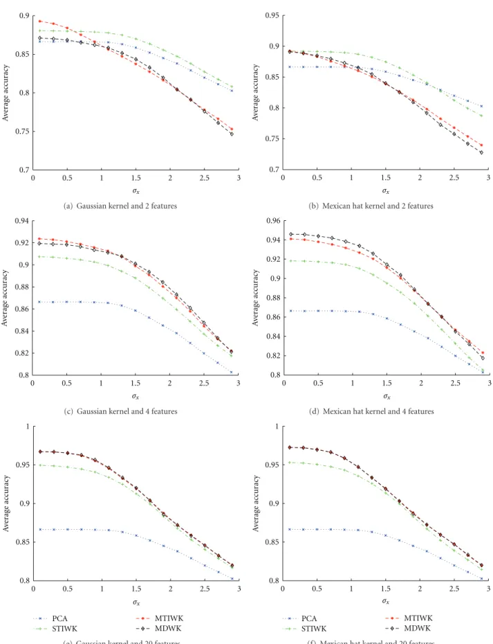
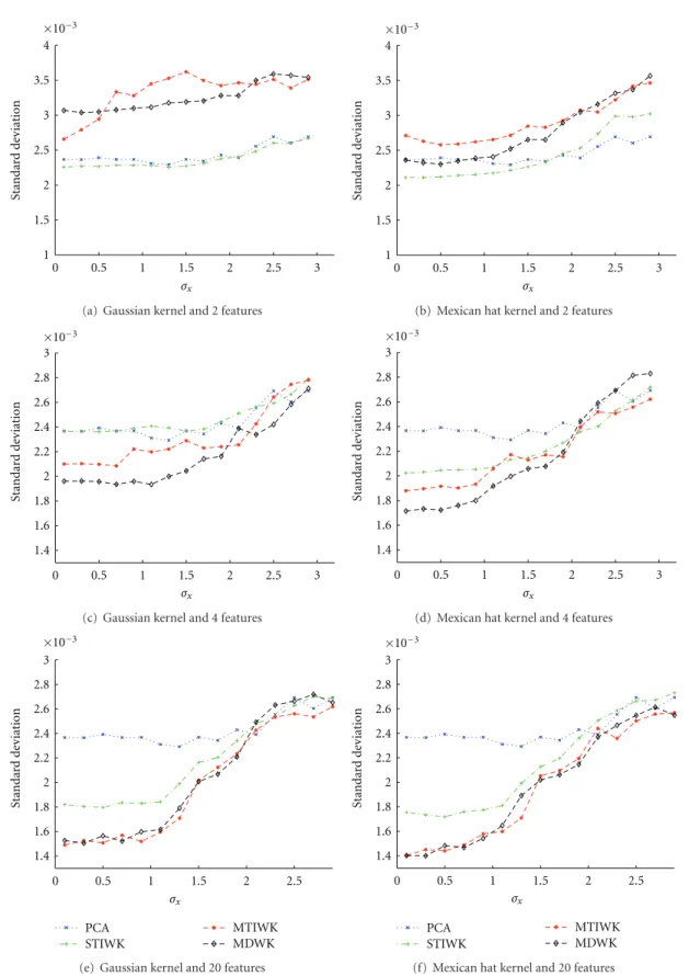
Besides a choice of the kernel and the determination of kernel parameters, feature dimension is also an important issue. The classification accuracy for a given data set may depend on a choice of feature dimension, requiring an investigation of how classification accuracy is related to the feature dimension. Estimates of the average classification accuracy rate and its sample standard deviation are obtained by applying the Monte Carlo method. The results of the average classification accuracy rates for a different number of retained features are reported in Figures 2(a)–2(f). The results of the change in behavior of the sample standard deviation for the average classification accuracy rate are presented in Figures 3(a)–3(f). Data classifications using both the FLD classifier and the feature extraction by PCA plus the FLD classifier have the worst performance for the simulated heterogeneous clustered data. Data classification using the multiscale WKPCA as feature extraction method shows the best performance. The feature extraction method using the multiscale WKPCA is less affected by the data variances than the feature extraction methods by PCA and the single-scale WKPCA.
7. Application to Epileptic EEG
Signal Classification
In order to demonstrate how the proposed methods perform when applied to real data, we use a set of EEG signals coming from healthy volunteers and from patients dur-ing seizure-free intervals. EEG signals are typically multi-scale and nonstationary in nature. The database is from the University of Bonn, Germany ( http://epileptologie-bonn.de/cms/front content.php?idcat=193), and has five sets, denoted as sets A, B, C, D, and E. We use only the sets A and E in our illustration. Set A consists of the signals taken from five healthy volunteers who were relaxed and in the awake state with eyes open. Signals in the set E were recorded from within the epileptogenic zone and contains only brain activity measured during seizure intervals. Each data group
A ver age ac cur acy 0.7 0.75 0.8 0.85 0.9 0 0.5 1 1.5 2 2.5 3 σx
(a) Gaussian kernel and 2 features
A ver age ac cur acy 0.7 0.75 0.8 0.85 0.9 0 0.5 1 1.5 2 2.5 3 σx 0.95
(b) Mexican hat kernel and 2 features
0.8 0.82 0.84 0.86 0.88 0.9 0.92 0.94 0 0.5 1 1.5 2 2.5 3 σx A ver age ac cur acy
(c) Gaussian kernel and 4 features
0.8 0.82 0.84 0.86 0.88 0.9 0.92 0.94 0 0.5 1 1.5 2 2.5 3 σx A ver age ac cur acy 0.96
(d) Mexican hat kernel and 4 features
A ver age ac cur acy 0.8 0.85 0.9 0 0.5 1 1.5 2 2.5 3 σx 0.95 1 PCA STIWK MTIWK MDWK
(e) Gaussian kernel and 20 features
PCA STIWK MTIWK MDWK A ver age ac cur acy 0.8 0.85 0.9 0 0.5 1 1.5 2 2.5 3 σx 0.95 1
(f) Mexican hat kernel and 20 features
Figure 2: Average classification accuracy rates when FLD classifier is used only (cyan plots) and when a feature extraction method plus FLD
classifier is used for 100 Monte Carlo simulations. The considered different types of feature extraction methods are PCA (blue plots), STIWK PCA (green plots), MTIWK PCA (red plots), and MDWK PCA (black plots) for the data simulated with different values ofσx.
0 0.5 1 1.5 2 2.5 3 1 1.5 2 2.5 3 3.5 4 σx Standar d de viation ×10−3
(a) Gaussian kernel and 2 features
0 0.5 1 1.5 2 2.5 3 1 1.5 2 2.5 3 3.5 4 σx Standar d de viation ×10−3
(b) Mexican hat kernel and 2 features
1.4 1.6 1.8 2 2.2 2.4 2.6 2.8 3 0 0.5 1 1.5 2 2.5 3 σx ×10−3 Standar d de viation
(c) Gaussian kernel and 4 features
1.4 1.6 1.8 2 2.2 2.4 2.6 2.8 3 0 0.5 1 1.5 2 2.5 σx ×10−3 3 Standar d de viation
(d) Mexican hat kernel and 4 features
PCA STIWK MTIWK MDWK 1.4 1.6 1.8 2 2.2 2.4 2.6 2.8 3 0 0.5 1 1.5 2 2.5 σx ×10−3 Standar d de viation
(e) Gaussian kernel and 20 features
PCA STIWK MTIWK MDWK 1.4 1.6 1.8 2 2.2 2.4 2.6 2.8 3 0 0.5 1 1.5 2 2.5 σx ×10−3 Standar d de viation
(f) Mexican hat kernel and 20 features
Figure 3: Sample standard deviations of average classification accuracy rates when FLD classifier is used only (cyan plots) and when a feature
extraction method plus FLD classifier is used for 100 Monte Carlo simulations. The considered different types of feature extraction methods are PCA (blue plots), STIWK PCA (green plots), MTIWK PCA (red plots), and MDWK PCA (black plots) for the data simulated with different values ofσx.
contains 100 single-channel scalp EEG segments of 23.6 second duration and each sampled at 173.61 Hz.
The problem we consider is the classification of normal signals (i.e., set A) and epileptic signals (i.e., set E). Since we deal with extremely high dimensional data (i.e.,d =4097), in order to make our classification task be computationally efficient, we first extract the signal features by calculating the wavelet approximation coefficients of each signal in data sets A and E. These signals are normalized before applying the wavelet transform using the Symlet 8 wavelet. We use the high-level wavelet decompositions due to the concerns of sparsity and the goal of obtaining high signal discrimination power. The samples of extracted features are shown in
Figure 4. Note that the coefficients of wavelet approximation around the two edges do not provide useful information for signal classification as those are affected by the edges of signals when the wavelet transform is applied. Only the coefficients of wavelet approximation within the central portion are considered as they are not affected by signal boundaries and have higher discrimination power compared to those around the edges. For example, at decomposition level 10, we obtained a set of three-dimensional features as the input of kernel PCA. Such low-dimensional feature in wavelet domain may not be sufficient to capture signal time-variability. Therefore, we consider additional two cases, that is, level 9 and level 8 wavelet decompositions. We select 7 and 11 features, which are corresponding to the wavelet approximation coefficients that ranges from the 8 to 14 and from 10 to 20 (within the central portion), respectively, for level 9 and 8 wavelet decompositions. We did not try a smaller level than 8 as it gives a very high dimensional feature set and the selection of features becomes difficult for those small levels.
As the input signals are normalized before the wavelet analysis, we eliminate the differences of the signal energy between groups. The high variability of extracted features reflects a high signal variability in original time domain. As we can see, the extracted features of normal signals are more fluctuated than the epileptic ones. This fact is coincided with the clinical findings about the rhythms of epileptic signals, which are more regularly fluctuated, that is, tends to be more deterministic. For all three cases that we considered, the WKPCA coupled with different kernels is applied to the wavelet approximation coefficients of signals and up to 20 principal components are extracted from WKPCA. The obtained results of classification accuracy, using different types of wavelet kernel and simple classifiers, are reported in Figure 5. As the high level of wavelet decomposition can only capture a very fine version of the signal, a level 10, which only gives the three-dimensional features, is not enough to capture signal time variability among groups. Although signal features are extended in PC space, it is important to retain the discriminative features from the original signals. Our study suggests that a level that slightly smaller than maximum allowed level is necessary to balance the trade-off between the classification performance and the sparsity of the input feature vector. The results shown in Figure 5also suggest that classification performance for this considered data set does not obviously depend on the
choice of kernel. Among all three cases considered, the best performance is obtained by using TI WKPCA with FLD classifier, which confirms our findings on the improvement of linearity of features using multiscale wavelet kernels. Thus, a non-linear classifier such as 1-NN may not necessarily outperform a linear classifier like FLD when WKPCA is used as a feature extraction method. This is because the linearity was improved by using the WKPCA and the 1-NN classifier performs better for clustered features than linear features. The classification accuracy is less affected by the feature dimension in PC space when the FLD classifier is used. However, TI WKPCA with 1-NN classifier achieves a higher accuracy when low-dimensional features are used for classification. This may suggest that it is beneficial to use the classification scheme that uses the multiscale wavelet KPCA plus a simple classifier including both linear and non-linear. The considered example demonstrates the applicability of the proposed method to multiscale data, and the proposed method could serve as an alternative approach to non-linear signal classification problems.
8. Conclusion and Discussion
This paper introduced a wavelet kernel PCA, in order to better capture data similarity measures in the kernel matrix. Multiscale wavelet kernels were constructed from a given mother wavelet function to improve the performance of KPCA as the feature extraction method in multiscale data classification. Based on analysis of the simulation data sets and the real data, we observed that the multiscale translation invariant wavelet kernel in KPCA has enhanced performance in feature extraction. The multiscale method for constructing a wavelet kernel in KPCA improves the robustness of KPCA in data classification as it tends to smooth out the locally modulated behavior caused by some types of mother wavelet. The application to real data was demonstrated through an EEG classification problem and the obtained results show the improvement of linearity after applying the multiscale WKPCA. Therefore, a simple linear classifier becomes suitable for classifying extracted features. This work focused on two important aspects: the first one was the construction of Mercer type wavelet kernel for kernel PCA and the second one was the investigation of the applicability of the proposed method.
The multiscale wavelet kernels proposed for the applica-tion in KPCA may also be useful for other kernel based meth-ods in pattern recognition, such as support vector regression, kernel discriminant analysis, kernel density estimation, or curve fitting. Many kernel-based statistical methods require the optimization of kernel parameters, which is usually com-putationally expensive for high dimensional data. Because of this, the use of multiscale kernels is impractical as the computational cost is dramatically increased with the increase of the number of kernel parameters of a multiscale kernel. Instead, multiscale wavelet kernels enable to narrow down the search for the values of kernel parameters. This is because a linear combination of a set of multiple kernel functions constructed from a mother wavelet function is
0 5 10 15 20 −1.5 −1 0 0.5 1
The ith wavelet coefficients
N o rmaliz ed wa ve let c o efficients
(a) Set A, at level 10
0 5 10 15 20 −1.5 −1 −0.5 0 0.5 1 N o rmaliz ed wa ve let c o efficients 1.5
The ith wavelet coefficients
(b) Set E, at level 10 −0.8 −0.6 −0.4 −0.2 0.2 0.4 0.6 0.8 0 5 10 15 20 0 25 N o rmaliz ed wa ve let c o efficients
The ith wavelet coefficients
(c) Set A, at level 9 −0.8 −0.6 −0.4 −0.2 0.2 0.4 0.6 0.8 0 5 10 15 20 25 0 N o rmaliz ed wa ve let c o efficients
The ith wavelet coefficients
(d) Set E, at level 9 −0.8 −0.6 −0.4 −0.2 0.2 0.4 0.6 0 5 10 15 20 25 0 30 N o rmaliz ed wa ve let c o efficients
The ith wavelet coefficients
(e) Set A, at level 8
−0.8 −0.6 −0.4 −0.2 0.2 0.4 0.6 0 5 10 15 20 25 0 30 N o rmaliz ed wa ve let c o efficients
The ith wavelet coefficients
(f) Set E, at level 8
Figure 4: The plots of coefficients of wavelet approximation of sample EEG signals at various wavelet decomposition level, that is, 10, 9, and 8.
5 10 15 20 0.4 0.5 0.6 0.7 0.8 0.9 Number of components Classification ac cur acy
(a) Gaussian kernel, at level 10
5 10 15 20 0.4 0.5 0.6 0.7 0.8 0.9 Number of components Classification ac cur acy 0.3
(b) Mexican hat kernel, at level 10
5 10 15 20 0.4 0.5 0.6 0.7 0.8 0.9 Number of components Classification ac cur acy
(c) Gaussian kernel, at level 9
5 10 15 20 0.4 0.5 0.6 0.7 0.8 0.9 Number of components Classification ac cur acy 0.3
(d) Mexican hat kernel, at level 9
Gaussian and FLD TI Gaussian wavelet and FLD Gaussian and 1-NN TI Gaussian wavelet and 1-NN 5 10 15 20 0.4 0.5 0.6 0.7 0.8 0.9 Number of components Classification ac cur acy
(e) Gaussian kernel, at level 8
5 10 15 20 0.4 0.5 0.6 0.7 0.8 0.9 Number of components Classification ac cur acy 0.3
Mexican hat and FLD TI Mexican hat wavelet
Mexican hat and 1-NN TI Mexican hat wavelet and 1-NN
and FLD
(f) Mexican hat kernel, at level 8
Figure 5: The classification accuracy with respect to different numbers of principal components retained under Gaussian and Mexican hat TI wavelet kernels, using the coefficients of wavelet approximation at various decomposition level. The classifiers used are FLD and 1-NN.
considered in this approach. It aims at capturing the multi-scale components of the data. However, since the multimulti-scale wavelet kernels are nonparametric, the performance of the kernel based methods using the multiscale wavelet kernels may not lead to an optimal solution to the problem.
Appendix
A. Proof of
Theorem 1
Let x1,. . ., xn∈Rdandr
1,. . .,rn∈R. It is sufficient to prove that the kernel matrix K is positive semi-definite. Since
n p n q rprqk(xp, xq) = n p n q rprq d i=1 J−1 j=0 N k=0 1 ajψ xi−bk aj ·ψ yi−bk aj = ⎛ ⎝n p rp d i=1 J−1 j=0 N k=0 1 √a jψ xp−b g aj ⎞ ⎠ × ⎛ ⎝n q rq d i=1 J−1 j=0 N k=0 1 √a jψ xq−b g aj ⎞ ⎠ = ⎛ ⎝n q rq d i=1 J−1 j=0 N k=0 1 √a jψ xq−b g aj ⎞ ⎠ 2 ≥0. (A.1) Therefore, the kernel defined in (7) is a Mercer kernel. This completes the proof.
B. Proof of
Theorem 2
Proof. By the Fourier condition theorem in [3], it is sufficient to prove that k(w)=(2π)−d/2 Rdexp −jwxk(x)dx≥0, (B.1)
for allw, where k(x)= d i=1 cos 5xi a exp −xi2 2a2 . (B.2)
Before we prove this fact, we first introduce the complex Morlet wavelet transform for a given signals(t). It is generally depicted as follows [28]: s(a,τ)= ∞ −∞s(t) 1 √ aexp −jk0t−τ a − (t−τ)2 2a2 dt, (B.3) where (1/√a) exp(−jk0((t −τ)/a)−(t −τ)2/2a2) is the
dilated and translated version of the complex Morlet mother wavelet function exp(−jk0t) exp(−t2/2) andτ,a ∈ R+ are
the translation and dilation factors, respectively. By taking s(t)=cos(wnt) and settinga=k0/w, (B.3) becomes
s(a,τ)= ∞ −∞cos(wnt) exp −jw(t−τ)−(t−τ) 2 2a2 √ w k0 dt = πk0 2w cos(wnτ) exp −(wn−w)2k02 2w2 + exp (wn−w)2k20 2w2 +jsin(wnτ) exp −(wn−w)2k20 2w2 −exp (wn−w)2k20 2w2 . (B.4) If we setτ=0,wn=5/a, andt=xiin (B.4), then we have
s(a, 0)=1 a ∞ −∞cos 5xi a exp−jwxi exp −x2i 2a2 dxi = πa 2 exp −(5/a−w) 2 a2 2 +exp (5/a−w)2a2 2 . (B.5) Observe that by substituting (B.2) into (B.1) we get
k(w)=(2π)−d/2 d i=1 ∞ −∞exp −jwixi− x 2 i 2a2 cos 5xi a dxi. (B.6) Using the results in (B.4) and (B.5),k(w) becomes
k(w)=2−d/2 d i=1 √ a × exp −(5/a−w) 2 a2 2 +exp (5/a−w)2a2 2 ≥0. (B.7) Therefore, the TI wavelet kernel constructed using the Morlet mother wavelet function is a Mercer kernel. This completes the proof.
Acknowledgments
S. Xie acknowledges the financial support from MITACS and Ryerson University, under MITACS Elevate Strategic Post-doctoral Award. P. Lio is supported by RECOGNITION: Relevance and Cognition for Self-Awareness in a Content-Centric Internet (257756), which is funded by the European Commission within the 7th Framework Programme (FP7).
References
[1] I. T. Jolliffe, Principal Component Analysis, Springer Science, New York, NY, USA, 2004.
[2] B. Scholkopf, A. J. Smola, and K. R. Muller, “Nonlinear com-ponent analysis as a kernel eigenvalue problem,” Neural Computation, vol. 10, no. 5, pp. 1299–1319, 1998.
[3] B. Scholkopf and A. J. Smola, Learning with Kernels—Support Vector Machines, Regularization, Optimization and Beyond, The MIT Press, Cambridge, Mass, USA, 2002.
[4] R. Rosipal, M. Girolami, L. J. Trejo, and A. Cichocki, “Kernel PCA for feature extraction and de-noising in nonlinear regression,” Neural Computing & Applications, vol. 10, no. 3, pp. 231–243, 2001.
[5] T. Hastie, R. Tibshirani, and A. Buja, “Flexible discriminant analysis by optimal scoring,” Journal of the American statistical Association, vol. 89, pp. 1255–1270, 1994.
[6] K. R. Muller, S. Mika, G. Ratsch, K. Tsuda, and B. Scholkopf, “An introduction to kernel-based learning algorithms,” IEEE Transactions on Neural Networks, vol. 12, no. 2, pp. 181–201, 2001.
[7] M. Zhu, “Kernels and ensembles: perspectives on statistical learning,” The American Statistician, vol. 62, no. 2, pp. 97–109, 2008.
[8] A. Karatzoglou, A. Smola, K. Hornik, and A. Zeileis, “Kernlab—An S4 package for kernel methods in R,” Journal of Statistical Software, vol. 11, no. 9, pp. 1–20, 2004.
[9] V. Vapnik, The Nature of Statistical Learning Theory, Springer, New York, NY, USA, 1995.
[10] V. Vapnik, Statistical Learning Theory, Wiley, New York, NY, USA, 1998.
[11] L. Zhang, W. D. Zhou, and L. C. Jiao, “Wavelet Support Vector Machine,” IEEE Transactions on Systems, Man, and Cybernetics B, vol. 34, no. 1, pp. 34–39, 2004.
[12] T. Takiguchi and Y. Ariki, “Robust feature extraction using kernel PCA,” in Proceedings of IEEE International Conference on Acoustics, Speech and Signal Processing (ICASSP ’06), pp. 509–512, Toulouse, France, May 2006.
[13] B. Scholkopf, A. Smola, and K. R. Muller, “Nonlinear com-ponent analysis as a kernel eigenvalue problem,” Technical Report 44, Max-Planck-Institut fur biologische Kybernetik Arbeitsgruppe Bulthoff, Tubingen, Germany, 1996.
[14] W. S. Chen, P. C. Yuen, J. Huang, and J. H. Lai, “Wavelet kernel construction for kernel discriminant analysis on face recognition,” in Proceedings of the Conference on Computer Vision and Pattern Recognition Workshops, p. 47, June 2006. [15] W. F. Zhang, D. Q. Dai, and H. Yan, “Framelet Kernels with
applications to support vector regression and regularization networks,” IEEE Transactions on Systems, Man, and Cybernetics B, vol. 40, no. 4, pp. 1128–1144, 2009.
[16] R. Opfer, “Multiscale kernels,” Technical Report, Institut fur Numerische und Angewandte Mathematik, Universitt Gottin-gen, 2004.
[17] A. Rakotomamonjy and S. Canu, “Frames, reproducing ker-nels, regularization and learning,” Journal of Machine Learning Research, vol. 6, pp. 1485–1515, 2005.
[18] P. Er¨ast¨o and L. Holmstr¨om, “Bayesian multiscale smoothing for making inferences about features in scatterplots,” Journal of Computational and Graphical Statistics, vol. 14, no. 3, pp. 569–589, 2005.
[19] T. Phienthrakul and B. Kijsirikul, “Evolutionary strategies for multi-scale radial basis function kernels in support vector machines,” in Proceedings of the Conference on Genetic and Evolutionary Computation (GECCO ’05), pp. 905–911, Wash-ington, DC, USA, June 2005.
[20] N. Kingsbury, D. B. H. Tay, and M. Palaniswami, “Multi-scale kernel methods for classification,” in Proceedings of IEEE
Workshop on Machine Learning for Signal Processing, pp. 43– 48, September 2005.
[21] F. Wang, G. Tan, and Y. Fang, “Multiscale wavelet support vector regression for traffic flow prediction,” in Proceedings of the 3rd International Symposium on Intelligent Information Technology Application (IITA ’09), vol. 3, pp. 319–322, Novem-ber 2009.
[22] H. Cheng and J. Liu, “Super-resolution image reconstruction based on MWSVR estimation,” in Proceedings of the 7th World Congress on Intelligent Control and Automation (WCICA ’08), pp. 5990–5994, June 2008.
[23] J. Wang and H. Peng, “Multi-scale wavelet support vec-tor regression for soft sensor modeling,” in Proceedings of the International Conference on Neural Networks and Brain (ICNNB ’05), vol. 1, pp. 284–287, October 2005.
[24] F. Han, D. Wang, C. Li, and X. Liao, “A multiresolution wavelet kernel for support vector regression,” in In Proceedings of the Third International Conference on Advances in Neural Networks (ISNN ’06), vol. 1, pp. 1022–1029, 2006.
[25] F. Wu and Y. Zhao, “Least square support vector machine on gaussian wavelet kernel function set,” in Proceedings of the 3rd International Conference on Advances in Neural Networks (ISNN ’06), vol. 3971 of Lecture Notes in Computer Science, pp. 936–941, 2006.
[26] S. Kadambe and P. Srinivasan, “Adaptive wavelets for signal classification and compression,” International Journal of Elec-tronics and Communications, vol. 60, no. 1, pp. 45–55, 2006. [27] I. Daubechies, Ten Lectures on Wavelets, SIAM, Philadelphia,
Pa, USA, 1992.
[28] H. C. Shyu and Y. S. Sun, “Underwater acoustic signal analysis by multi-scaling and multi-translation wavelets,” in Wavelet Applications V, vol. 3391 of Proceedings of SPIE, pp. 628–636, Orlando, Fla, USA, April 1998.