Learning and Searching Methods for Robust, Real-Time Visual Odometry.

(1)

Learning and Searching Methods for

Robust, Real-Time Visual Odometry

by

Andrew Ross Richardson

A dissertation submitted in partial fulfillment of the requirements for the degree of

Doctor of Philosophy

(Computer Science and Engineering) in the University of Michigan

2015

Doctoral committee:

Associate Professor Edwin Olson, Chair Associate Professor Ryan M. Eustice Professor Benjamin Kuipers

(2)

(3)

List of Figures

Figure

1.1 The team of ground robots that formed the University of Michigan’s entry in the MAGIC 2010 robotics competition . . . 2 1.2 Global, multi-robot maps from the MAGIC 2010 robotics competition 3 2.1 Illustration of the ideal pinhole camera model . . . 7 2.2 A distorted camera image and an equivalent image with distortion

removed . . . 8 2.3 Images before and after resampling with a homography . . . 9 2.4 Epipolar geometry and stereo rectification . . . 10 2.5 Color and corresponding dense disparity image from Scharstein et al. 11 2.6 Feature detections for three common image feature categories . . . . 12 3.1 Examples of convolutional filters for image feature detection . . . 17 3.2 Basis sets for the Discrete Cosine Transform (DCT) and Haar Wavelet

Transform . . . 21 3.3 Illustrations of frequency-domain filter constraints for 8_×8 filters . . 22 3.4 Ground truth camera motion reconstruction using AprilTags . . . 25 3.5 Images from the four datasets used for feature detector learning . . . 27 3.6 Reconstruction of the ground-truth camera trajectories and landmark

positions . . . 28 3.7 Time comparison between FAST-9 and an 8_×8 convolutional filter

feature detector. . . 29 3.8 Mean reprojection error for the best convolutional filter sampled so far

(running minimum error) over 5,000 samples . . . 31 3.9 Visualization of the best learned convolutional filter for each

combina-tion of dataset and sampling type . . . 31 3.10 Histogram of mean reprojection errors for three filter generation

meth-ods on the conference room dataset . . . 32 3.11 Distributions of block-diagonal filter reprojection errors for filters with

(6)

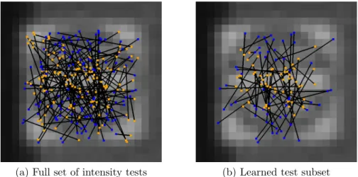
4.1 Illustration of BRIEF and TailoredBRIEF intensity tests for an image of a road sign . . . 37 4.2 Intensity tests on a road sign image patch under simulated viewpoint

changes . . . 42 4.3 Descriptor matching error distributions for example patches using BRIEF

and TailoredBRIEF . . . 43 4.4 Sample images from the affine region detector dataset . . . 47 4.5 Percentage of TailoredBRIEF test results that are suppressed as a

func-tion of the sample accuracy threshold . . . 48 4.6 Precision-Recall curves for the Wall dataset, image 1 versus 3 . . . . 49 4.7 Precision-Recall curves for all datasets and images . . . 51 5.1 Edge-feature matching with and without motion constraints . . . 56 5.2 Sparse feature detections and depth map for 1D features detected with

a calibrated stereo system . . . 57 5.3 Illustration of the feature detectors evaluated in this work . . . 59 5.4 Example 1D convolutional filter detections and matches on the Midd1

and Rocks1 images from the 2006 Middlebury dense disparity dataset 62 5.5 Plots of runtime vs. percentage of inliers with a constant number of

matches per plot . . . 64 5.6 Percent of match inliers when a 1-pixel horizontal tolerance is used to

prevent incorrect penalization of features on depth discontinuities . . 65 5.7 Runtime and percent of inliers with 2500 matches and additive noise 68 5.8 Runtime and inlier percentage for 2500 matches with blurred images . 68 5.9 Illustration of the PAS search tree for a one-dimensional search . . . . 73 5.10 Visualization of the perspective motion bound . . . 76 5.11 Translation-image pyramid in a synthetic environment . . . 78 5.12 Translation-image pyramid using real features . . . 78 5.13 Comparison of the first order pixel motion bound for PAS-6D and a

sweep over 6-DoF transformations . . . 79 5.14 Transformation-image pyramid for PAS-6D . . . 80 5.15 Simulation environment for PAS using a deliberately-drifting pose

es-timate . . . 81 5.16 Mean and max pose error for three configurations against the true,

simulated pose as the frame rate is varied . . . 81 5.17 Mean pose error for three configurations against the true, simulated

pose as the simulated gyro drift rate is varied . . . 82 5.18 Visual odometry with PAS vs. LIDAR-based SLAM for a 3 minute

indoor trial . . . 85 5.19 Accumulated edge features after alignment with PAS . . . 85 5.20 Example image from the KITTI dataset with detected features and

(7)

(8)

List of Tables

Table

3.1 Motion estimation testing error (pixels) on each dataset using learned feature detectors and baseline methods . . . 34 4.1 Ranges for randomly-sampled viewpoint change parameters . . . 48 4.2 Area under the Precision-Recall curves for all datasets and images . . 52 4.3 BRIEF and TailoredBRIEF runtimes for each stage of description and

matching . . . 54 5.1 Time required to generate an average of 2,500 matched features on the

Middlebury dataset using the SSE-optimized 1D convolutional detector 66 5.2 Average computation time for image preprocessing and stereo feature

matching . . . 83 5.3 Parameter sweep for PAS to find the best update rate and search

res-olution . . . 84 5.4 Comparison of methods for motion estimation using two frame rates

on a 3 minute indoor log . . . 86 5.5 Parameters for PAS evaluation on the KITTI dataset . . . 87 5.6 Comparison of PAS translation estimates compared to ground truth.

Values represent averages over all sequential motion estimates . . . . 87 5.7 Comparison of performance for PAS and a subset of single-core

(9)

List of Acronyms

AVX Advanced Vector Extensions

CPU Central Processing Unit DCT Discrete Cosine Transform DoF Degree of Freedom

DOG Difference Of Gaussians FFT Fast Fourier Transform FPS Frames Per Second

GPS Global Positioning System GPU Graphics Processing Unit IC Integrated Circuit

ICP Iterative Closest Point IMU Inertial Measurement Unit

MEMS Microelectromechanical System ML Maximum Likelihood

MSEMean-Squared Error

PASPerspective Alignment Search POPCNT Population Count

RANSACRandom Sample And Consensus ROC Receiver Operating Characteristic SAD Sum of Absolute Differences SIMD Single Instruction Multiple Data

SLAM Simultaneous Localization And Mapping SSE Streaming SIMD Extensions

USB Universal Serial Bus VIO Visual-Inertial Odometry

(10)

VO Visual Odometry VSLAM Visual SLAM XOR Exclusive Or

(11)

Abstract

Accurate position estimation provides a critical foundation for mobile robot percep-tion and control. While well-studied, it remains difficult to provide timely, precise, and robust position estimates for applications that operate in uncontrolled environ-ments, such as robotic exploration and autonomous driving. Continuous, high-rate egomotion estimation is possible using cameras and Visual Odometry (VO), which tracks the movement of sparse scene content known as image keypoints or features. However, high update rates, often 30 Hz or greater, leave little computation time per frame, while variability in scene content stresses robustness. Due to these challenges, implementing an accurate and robust visual odometry system remains difficult.

This thesis investigates fundamental improvements throughout all stages of a vi-sual odometry system, and has three primary contributions: The first contribution is a machine learning method for feature detector design. This method considers end-to-end motion estimation accuracy during learning. Consequently, accuracy and robustness are improved across multiple challenging datasets in comparison to state of the art alternatives. The second contribution is a proposed feature descriptor, TailoredBRIEF, that builds upon recent advances in the field in fast, low-memory descriptor extraction and matching. TailoredBRIEF is an in-situ descriptor learning method that improves feature matching accuracy by efficiently customizing descrip-tor structures on a per-feature basis. Further, a common asymmetry in vision system design between reference and query images is described and exploited, enabling ap-proaches that would otherwise exceed runtime constraints. The final contribution is a new algorithm for visual motion estimation: Perspective Alignment Search (PAS). Many vision systems depend on the unique appearance of features during matching, despite a large quantity of non-unique features in otherwise barren environments. A search-based method, PAS, is proposed to employ features that lack unique ap-pearance through descriptorless matching. This method simplifies visual odometry

(12)

pipelines, defining one method that subsumes feature matching, outlier rejection, and motion estimation.

Throughout this work, evaluations of the proposed methods and systems are car-ried out on ground-truth datasets, often generated with custom experimental plat-forms in challenging environments. Particular focus is placed on preserving runtimes compatible with real-time operation, as is necessary for deployment in the field.

(13)

Chapter 1 Introduction

Real-time position estimation is a fundamental problem in robotics that enables appli-cations such as mapping, planning, and control. Estimates of the motion over a short time horizon, on the order of a few seconds, enable sensor data to be accumulated to provide a more detailed description of the surrounding environment or to distinguish between the static and dynamic parts of the scene. Estimates of the motion over a longer horizon, on the order of minutes or hours, allow robots to collaborate on large map-building tasks and minimize duplication of effort. Low-latency, local position estimates are important for stable, high-speed control, while low-rate, global position estimates are critical to relate prior map data, such as reference trajectories or scene structure, to the robot’s current state, such as its current position or live sensor data. For amobile robot defined by its ability to move throughout the world, knowledge of its own motion is critical.

Robustly estimating a mobile robot’s position is difficult. Dead-reckoning with a combination of wheel odometers, gyroscopes, and accelerometers can provide satis-factory estimates for short-term goals in favorable conditions. However, continuous integration alone of the noisy and biased velocity and acceleration measurements available from consumer-grade devices leads to position drift that is unsuitable for sustained navigation. A solution to position estimate drift popular since antiquity is celestial navigation — position estimation on the surface of the Earth using observa-tions of the stars [1]. A host of related approaches use observable landmarks whose positions are known (or assumed) to be fixed, through which drift in a dead-reckoned position estimate can be observed and rejected. Alternatively, if the landmarks are reliably observed and readily detected, position estimates can be computed without the use of additional measurements.

(14)

The Global Positioning System (GPS) is one such landmark-based solution [2]. It uses active electronic beacons, calculating position through inference involving the time of flight for each signal. GPS is widely available, but it is sensitive to ionospheric distortions and the reflection of signals within urban canyons. It fails when line-of-sight paths to four or more satellites are not available, as inside tunnels or buildings. This poses a problem for robots operating in mixed indoor/outdoor environments and autonomous vehicles operating in cities.

Figure 1.1 shows an example of a robotic system that motivated this work and operated in the challenging physical environments described previously. This system, the University of Michigan’s winning entry to the MAGIC 2010 robotics challenge, highlighted the need for position estimation systems robust to rough terrain in un-known environments.

Figure 1.1: The team of ground robots that formed the University of Michigan’s entry in the MAGIC 2010 robotics competition. ➞ 2012 Wiley Periodicals, Inc.

In MAGIC 2010, the University of Michigan’s 14 small (26 inch_×20 inch) ground robots autonomously mapped an urban fairgrounds with limited, remote human over-sight [3]. These robots, with a top speed of 1.2 m/s, explored this 500 m _× 500 m mixed indoor-outdoor course in 3.5 hours while stopping for numerous reconnaissance objectives. A centralized ground station coordinated the multi-robot exploration and mapping tasks, fusing individual maps derived from robots’ LIDAR data into a shared, global map.

This difficult challenge combined multi-robot mapping, planning, perception and control. These maps enabled autonomous, coordinated exploration in this unknown environment by providing a unified representation for multi-robot planning and for avoidance of simulated threats. However, these maps possessed local distortions

(15)

re-sulting from wheel odometry inaccuracies, which occurred as a result of the uneven terrain. Figure 1.2 shows an aerial camera view and the maps estimated during the competition.

(a) Aerial view (b) Live mapping results (Phases 1-3)

Figure 1.2: Global, multi-robot maps from the MAGIC 2010 robotics competition [3]. The course was divided into threephases of increasing difficulty, as shown in (b). Some geometric distortion is present in the final live map estimates due to inaccurate odometry estimates. Note the distortion in the bottom-left of Phase 1 or top-right of Phase 2. ➞ 2012 Wiley Periodicals, Inc.

Camera-based approaches to motion estimation have been well-studied [4, 5, 6, 7] and can make use of low-cost sensors and compute platforms. Many of these methods are formulated in terms of image feature detection, description, and matching to decompose the image-based motion estimation problem. Features, visual landmarks corresponding to geometric primitives such as corners, are detected in the image by selecting local maxima of a response function. This reduces the dense, regular array of intensity values in the image to a small number of discrete elements with known geometric properties, such as position or orientation. Between multiple images, features are matched by selecting correspondences that minimize an error function between two feature descriptors. These descriptors summarize the image appearance surrounding the feature in order to provide robustness to phenomena that affect the appearance of the image as a whole, such as viewpoint or lighting change.

Visual Odometry (VO) is a method that tracks the frame-to-frame motion of features to provide a high-rate estimate of the incremental camera motion [6]. The feature correspondences between frames provide the constraints used to simultane-ously solve for the 3D feature positions and the 6 Degree of Freedom (6-DoF) camera

(16)

motion. One camera is sufficient given enough correspondences, but there are ad-vantages to multi-camera approaches. In the stereo case, using two cameras with an overlapping field of view, the position of each image feature relative to the cameras may be computed for every image pair [8], given that correct feature correspondences have been formed.

Visual motion estimation methods are capable of providing accurate, high-rate position estimates in conditions where dead-reckoning and GPS fail. Yet, implement-ing such a system remains difficult due to trade-offs between runtime, accuracy, and reliability. Further, these trade-offs are present at each stage in a motion estima-tion pipeline — the type of features detected, the representaestima-tion used to describe them, and the methods to compute correspondences and resolve the camera motion all impact the performance of the system.

This thesis develops unique approaches for detection, description, and motion estimation in the visual odometry context. An emphasis is placed on real-time, stereo approaches using low-cost sensors and operation in challenging environments.

1.1 Thesis overview

Building a visual odometry system remains challenging because of confounding fac-tors such as environmental variability and because of the trade-offs between detection repeatability, matching accuracy, runtime, frame rate, memory overhead, and simplic-ity. This thesis improves the state of the art by investigating new methods for every stage of a feature-based visual odometry pipeline and through a unique focus on both descriptor-based and descriptorless visual motion estimation. An emphasis is placed on preserving runtimes compatible with high frame rate, real-time use, as is expected for robots operating in the field.

The key contributions of this thesis are:

❼ Chapter 3: A method for feature detector design that, in an offline setting, learns a detector to maximize the accuracy of a target visual odometry pipeline using ground-truth, camera-in-hand datasets in everyday, 3D environments ❼ Chapter 4: A method for online feature descriptor learning that effectively

performs per-feature customization of the descriptor sampling pattern. This method, TailoredBRIEF, improves upon recent advances in intensity-comparison

(17)

descriptors by addressing the sensitivity of specific comparisons to small changes in viewpoint, increasing the overall feature matching accuracy

❼ Chapter 5: An alternative, search-based formulation for sparse, feature-based visual odometry. This approach, Perspective Alignment Search (PAS), effi-ciently utilizes indistinct visual features that are plentiful in otherwise feature-deficient indoor environments. These indistinct edge features would confound descriptor-based matching in a traditional odometry application, but are suc-cessfully used in PAS through a descriptorless formulation and whole-scene alignment objective

(18)

Chapter 2 Background

Position estimation using one or more cameras requires an understanding of the math-ematical model used to describe image formation and the algorithms used to transform the raw image data into a form suitable for motion estimation.

2.1 Image formation

The dominate model for image formation in computer vision is the pinhole camera model [8]. In the pinhole model, rays of light pass through a infinitesimally small hole, or aperture, in a thin medium and strike an imaging plane. This is considered a

perspective projection. The image is formed by measuring the light received for each pixel on the plane.

A small aperture is necessary to create a clear, sharp image. Without an aperture, diffuse reflections would scatter light from a single source across the image plane, resulting in measurements at each pixel without a unique source. The aperture serves to permit only a subset of the available light and generate a coherent image.

The pinhole camera model can be described in terms of the position of a 3D point,

X = [X, Y, Z]T_{, and the camera parameters, including the focal lengths (}_f

x, fy) and

optical center (cx, cy). Projecting through the pinhole model yields a coordinate in

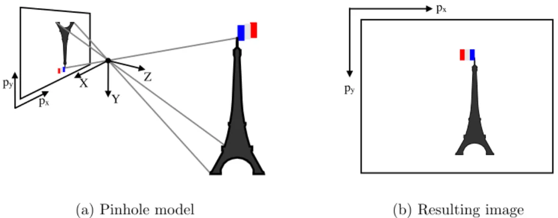
pixels, (px, py). An illustration of this model is shown in Figure 2.1.

px =fx X Z +cx (2.1) py =fy Y Z +cy (2.2)

(19)

Frequently, the pinhole model in Equations 2.2 is instead described in terms of the intrinsics matrix, K,

K=    fx 0 cx 0 fy cy 0 0 1    (2.3)

which relates the camera frame and image coordinates for a point X = [X, Y, Z]T linearly, up to scale (subject to the constraint thatpw = 1).

[px, py, pw]T =K·X (2.4)

In practice, most cameras deviate from the pinhole camera model. Small apertures yield crisp images, but also permit little light to strike the image sensor. Consequently, most cameras use a lens to focus additional light into a crisp image. This yields an image with less noise, but results in image distortion whereby the image cannot be described by the pinhole camera model, alone [8]. Once distorted, straight lines as projected under the pinhole camera model appear bent across the image. For problems in metrical computer vision, understanding and mitigating the effects of lens distortion is necessary to produce accurate and meaningful results.

px

py X

Y Z

(a) Pinhole model

px

py

(b) Resulting image

Figure 2.1: Illustration of the ideal pinhole camera model. Relative to the scene, the image appears flipped on the image plane as a consequence of light passing through the pinhole camera aperture

Imaging lenses are engineered to be axially symmetric about the principal axis. When mounted with the axis of symmetry perpendicular to the image plane, it is typically sufficient to express the image distortion as a polynomial function of a

(20)

dis-tance from the optical center of the image or, similarly, as a function of the angular deviation from the principal axis. The parameters of this polynomial, as well as the focal length and focal center parameters, make up what are called the intrinsic pa-rameters of the camera. In addition, the extrinsic parameters describe the position of the camera with respect to the origin in some coordinate system, be it another camera, the center of a robot, or a map. These intrinsic and extrinsic parameters can be estimated in a process known as camera calibration [9, 10, 11, 12]. Camera cali-bration is a field unto itself, and we have demonstrated expertise in this area through the development of a state-of-the-art camera calibrator known as AprilCal [12].

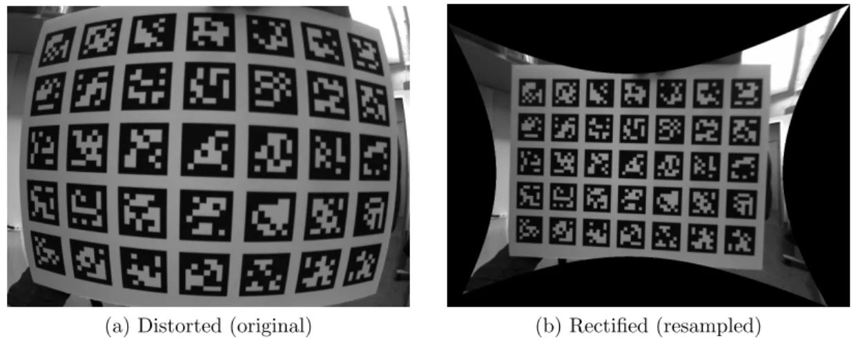
Once all intrinsics parameters are known, the effects of lens distortion can be properly predicted by an application. Alternatively, the distortion can be removed using image rectification, which resamples the image according to a distortion-free camera model. An example of a distorted and rectified image is shown in Figure 2.2. Note that the straight lines on the rectangular grid appear straight in the rectified image, as is easily predicted by the pinhole model.

(a) Distorted (original) (b) Rectified (resampled)

Figure 2.2: A distorted camera image and an equivalent image with distortion removed. Bilinear interpolation is used to resample a rectified image from the original, distorted version.

The perspective imaging process loses an important quantity — scene depth. While ray direction for each pixel is determined through calibration, the distance to the scene along the ray is unknown. This depth can be recovered if more is known about the geometry of the scene, or if multiple views are available.

(21)

a two-dimensional homography. The 3_×3 homography matrix,H, relates two corre-sponding homogenous points in the image,x andx′_{, such that} _x′ ₌_Hx_{, up to scale.}

Homographies can be used to create synthetic, ortho-rectified views of a plane, or to map between image coordinates for two images of a planar scene. Figure 2.3 shows an image of a planar roadway and the corresponding top-down, orthographic view computed by resampling the original image with a homography.

(a) Perspective view (b) Resampled

Figure 2.3: Images before and after resampling with a homography. A top-down view of a painted street is synthetically computed by sampling uniformly-spaced values using a homography.

In the case of two cameras, the unknown depth of a point in the first image projects into the second image as an epipolar line [8]. Thus, the distance to a point observed in the first image can be recovered if the corresponding point is found in the second image. This search along the epipolar line is simplified through stereo rectification [8]. In stereo rectification, a pair of images are resampled so that lens distortion is removed and the epipolar lines lie horizontally [13]. This reduces the search along an arbitrary epipolar curve or line in the second image to a search along the corresponding row. Figure 2.4 illustrates these scenarios.

The difference inxcoordinates for a point in two stereo-rectified images,px2−px1,

is known as the disparity. Recovery of the full depth map for a stereo image pair is known as dense disparity estimation, sometimes called dense stereo. Quantitative evaluation of many dense disparity estimation methods is available from Scharstein et al. [14, 15, 16, 17], including the well-known Semi-Global Matching (SGM) approach from Hirschm¨uller [18]. Figure 2.5 shows a sample image and ground-truth depth map.

For many motion estimation systems, the dense solution is not required andsparse stereo methods are used instead.

(22)

e1 e2 X px1 px2 c1 c2 l1 l2 px1 px2 l1 l2

Figure 2.4: Epipolar geometry and stereo rectification. (Top) Illustration of epipolar ge-ometry. The camera centersc1 and c2 are connected by a line through the epipolese1 and

e₂ _{called the}_baseline_{. The projections of the 3D point} X _{lies on the epipolar lines} l₁ _and l₂_{. (Bottom) Through stereo rectification, the image is resampled so that the epipolar lines}

are horizontal and occupy corresponding rows. This allows algorithms to operate on only corresponding scanlines when performing disparity estimation.

2.2 Image features

Images are composed of a dense, regular array of intensity samples, typically totaling hundreds of thousands to millions of samples. To deal with such a large amount of data, feature-based methods reduce the image to a set of discrete image primitives, such as points, lines, or uniform regions. The presence and position of these primitives, or image features, are extracted through the use of afeature detector. Local feature appearance is summarized using a feature descriptor. Detectors and descriptors are designed to provideinvariant performance against various physical phenomena, yield-ing repeatable detection or identical descriptions despite scene lightyield-ing or viewpoint variations.

A number of invariant properties are commonly described in the literature: ❼ Lighting: Invariance to additive offsets and multiplicative scale factors in

recorded lighting levels

❼ Translation: Invariance to feature position within an image

❼ Scale: Invariance to size changes for image features (fixed aspect ratio). This is a consideration for region (blob) features with defined extents. Scale-invariant

(23)

Figure 2.5: Color and corresponding dense disparity image from Scharstein et al. [16]. Reproduced with permission.

detection reports a local extrema in a joint position and scale space. Scale-invariant description summarizes an image area that varies in size proportional to a feature’s scale

❼ Rotation: Invariance to in-plane rotation of the image. For descriptors, the dominant orientation may be estimated to enable extraction of a rotation-corrected descriptor

❼ Affine: Invariance to the combined effects of translation, rotation, and scaling, particularly with a variable aspect ratio. In practice, it is used to increase robustness to out-of-plane rotation

Features are categorized by the type of geometric primitive represented. Broadly speaking, point features require the least computation and thus incur the lowest run-times, while blob features possess the greatest level of invariance. Consequently, point features are more common in high-rate video applications such as visual odometry, while blob features are used frequently for visual search, object recognition, place recognition, and so on. Figure 2.6 shows examples of the three feature categories.

❼ Points & Corners: Harris [19], FAST [20, 21], convolutional filters [22, 23], or ORB [24]

❼ Lines: Canny edge detector [25]

(24)

(a) Point features (b) Line features (c) Blob features

Figure 2.6: Feature detections for three common image feature categories. Detections denoted by orange points, lines, or circles

In this thesis, the term feature is used to refer to a detected image primitive, which has an associated image and position, and which optionally has an associated descriptor. The portion of the image immediately surrounding a feature detection is a pixel patch, which is sometimes used directly as a feature descriptor. As works in the literature vary in focus on one or both aspects of the detection and description problems, a categorization for a selection of methods is provided below.

❼ Detector-only: Harris [19], FAST [20, 21], CenSurE [28], learned detectors from Trujillo and Olague [30], convolutional filters [22, 23]

❼ Descriptor-only: Pixel patch, DAISY [31], learned descriptors from Brown et al. [32], BRIEF [33]

❼ Detector & Descriptor: SIFT [26], SURF [27], ORB [24], BRISK [34] The performance of feature detectors and descriptors are analyzed by a number of metrics. These metrics includerepeatability, the degree to which features detected in a reference image are detected in other images of the same content, precision, the fraction of computed matches that are true correspondences, and recall, the frac-tion of features for which true correspondences exist that were matched correctly. Other criteria include computation time for various stages (detection, description, and matching), and the memory footprint required to store descriptors or transfer them throughout the system.

(25)

2.3 Feature-based methods

Image features are useful in a wide range of applications, including Visual Odom-etry (VO) [6, 35, 36, 23], Visual Simultaneous Localization And Mapping (Visual SLAM) [4, 5, 7, 37], bundle adjustment [38, 8, 39], place recognition [40], object recognition [41], and dense reconstruction [31].

Motion and location estimation are a common theme throughout visual odometry, visual SLAM, bundle adjustment, and place recognition. These methods differ in scope — in visual odometry, only the frame-to-frame camera motion is estimated [6, 22], while in visual SLAM and bundle adjustment, the joint estimation problem is solved using many camera positions and many more features. In RSLAM, Mei et al. presented a constant-time, large-scale mapping method to build visual maps online in a relative coordinate frame [7], balancing metrical accuracy and the scalability of map updates as the mapped area grows. In the bundle adjustment domain, Agarwal et al. presented a method to perform city-scale visual mapping offline using images scraped from the web [38].

The limited time-horizon of visual odometry and sliding-window visual SLAM formulations provide a mechanism for runtime control at the expense of global pose accuracy. While Agarwal et al.’s method was designed to reconstruct a city offline, across many cores, and over the course of a day [38], many visual odometry and visual SLAM methods are intended for in-situ, real-time use [6, 22, 7, 37].

Alternative formulations to live egomotion estimation are live localization and place recognition. Such methods make use of prior maps which can be built ahead of time, offline, using more data, time, and computational resources than would be available online. At runtime, these methods estimate the current map position, either globally, which is known as the “kidnapped robot problem”, or locally, using available pose priors. Consequently, visual odometry and visual localization are complemen-tary, as visual localization can reject the slow pose drift incurred by a visual odometry application. One example of place recognition is FAB-MAP — an appearance-based, bag-of-words visual place recognition application that recursively estimates the proba-bility of revisiting a location given the re-observation of quantized visual features [40]. The precise usage of image features differs by application. In visual odometry, high frame rates and constant velocity assumptions limit the possible feature motion within the image, which allows less distinctive image features to be used. Some applications

(26)

simply perform a dense search about the pose prior using a pixel patch descriptor [5]. Closing loops in visual SLAM, however, involves greater relative position uncertainty. Consequently, features with greater invariances are typically used, such as the scale-invariant SURF features used in FAB-MAP [40].

A typical visual odometry application tracks image features through a video and estimates the camera motion and feature positions using Least Squares or a similar method. In the stereo camera case, the feature positions can be estimated for every image pair, as the intrinsic and inter-camera extrinsic parameters are known. The camera motion can then be initialized by aligning the two 3D point sets with a method such as that by Horn [42] and refined iteratively, or through a Perspective-n-Point (PnP) method such as Lepetit et al.’s EPnP [43]. Many variations on this approach have been described in the literature. For example, some stereo systems use only one image whenever possible [44], to reduce computational load. Ma et al. fuse data from a stereo camera, legged robot odometry, and a tactical-grade IMU [45]. Howard uses inlier detection based on dense disparity images [35], computing inliers before estimating the inter-frame motion.

Achieving robustness for these systems is critical, as pose estimation forms the foundation of the rest of the system. The feature matching process almost always gen-erates a small number of incorrect correspondences, however, as multiple features may have similar appearance. Incorrect correspondences, oroutliers, can have a significant impact on the estimated motion. One way to make these methods robust is through an outlier rejection stage, such as Random Sample And Consensus (RANSAC) [46]. In RANSAC, the minimum set of correspondences needed to compute a joint error function are repeatedly drawn so that the degree of consensus, the agreement with the resulting model, can be computed for each hypothesis. Given that the majority of correspondences are inliers, hypotheses formed only of correct correspondences will yield a low error, allowing outliers to be detected and discarded.

Speed and efficiency are a high priority for pose estimation, as many robots require real-time operation in the field using limited computational resources. Modern CPU architectures include Single Instruction Multiple Data (SIMD) vector instruction sets to compute multiple results in parallel, which is known as data-level parallelism. These instructions are often used for scientific and multimedia applications. They can also be used to boost the performance of visual tracking systems, as has been demonstrated in recent work [22, 33]. Examples of SIMD processor extensions include

(27)

Intel’s Streaming SIMD Extensions (SSE) versions 1-4, Advanced Vector Extensions (AVX), AVX2, AVX-512, and ARM’s NEON extensions. In this thesis, we make use of Intel SSE and ARM NEON extensions.

2.4 Dense and correlative methods

Feature-based methods are not the only approach for camera and LIDAR position estimation. Dense and correlative methods can be applied in many situations.

Dense methods have found recent popularity with the parallelism available through a Graphics Processing Unit (GPU). Newcombe et al. proposed DTAM, a method for real-time, dense mapping with a single camera [47]. DTAM performs many-view dense disparity estimation, minimizing the average, absolute photometric error over many short-baseline views. In KinectFusion, a GPU variant of the Iterative Closest Point (ICP) method was applied to a stream from a depth camera to alternately align and update a voxel-based surface representation [48]. Wolcott and Eustice recently proposed a method for camera-based localization to a LIDAR-derived intensity map, maximizing the mutual information between a live camera image and synthetic views generated on a GPU [49].

Correlative methods have also been used for alignment of LIDAR data. Levinson, Montemerlo, and Thrun presented a particle-filter method for LIDAR localization into a ground-plane intensity map [50]. Olson detailed a multi-scale approach for correlative “scan-matching” of planar LIDAR data that is robust to local minima [51], unlike iterative alternatives like ICP.

(28)

Chapter 3 Feature detector learning

1

Most feature detectors described in the literature were designed by hand. This man-ual design process allows the designer to leverage intuition about the problem and explore a large, non-linear design space. While flexible, this approach to the design and export of stand-alone feature detectors overlooks the differing requirements of target applications. This chapter proposes and evaluates a method for automati-cally learning feature detectors with the target application, a stereo visual odometry system, “in-the-loop”. The goal of this work is to generate a feature detector that maximizes the accuracy of the motion estimation pipeline, given the design decisions in place in the implementation of that system. This approach allows us to thoroughly explore the space of possible feature detectors and better understand the properties of the top-performing detectors.

We propose to learn fast and effective feature detectors by restricting the detector design space to aconvolutional filter parameterization. Convolutional filters make up an expressive space of feature detectors, yet possess favorable computational prop-erties, including the ability to leverage SIMD instruction sets. The specific target application in this work is stereo visual odometry, which requires fewer feature invari-ances than an application that lacks any motion prior or continuity. Unlike feature detection and matching evaluations limited to planar environments, these detectors are learned on real video sequences in everyday, 3D environments. This approach ensures the relevance of the learned results.

Learning these high-performance feature detectors requires a good source of train-ing data, which can be difficult or expensive to obtain. We detail our method for

gen-1_➞

2013 IEEE. Adapted with permission, from Andrew Richardson and Edwin Olson, “Learning Convolutional Filters for Interest Point Detection,” May 2013.

(29)

Figure 3.1: Examples of convolutional filters for image feature detection. Hand-selected filters include the corner and point detectors used by Geiger et al. [22] (top, both) and a Difference-of-Gaussians (DOG) filter (bottom left) like those used for scale-space search in SIFT [26]. The proposed method automatically learns convolutional filters for feature detection. (Bottom right) The most accurate filter from this work.

erating ground truth data — instrumenting an environment with 2D fiducial markers known as AprilTags [52]. These markers are robustly detected with low false-positive rates, allowing us to extract features with known, global data association. These constraints allow us to solve for the global poses of all cameras and markers, which is used to evaluate motion estimates computed using only natural visual features. Im-portantly, this global reconstruction is used to reject any feature detections present on or near AprilTags, ensuring that the learn process is not biased by the presence of fiducial markers.

The feature detectors learned with our method are efficient and accurate. Pro-cessing times are comparable to FAST [20], a decision-tree formulation for corner detection, and reprojection errors for stereo visual odometry are lower than those with FAST in most cases. In addition, because our filters use a simple convolutional structure, processing times are reduced by both increases in CPU clock rates and SIMD vector instruction widths.

The main contributions of this work are:

1. A framework for learning a feature detector designed to maximize performance of a specific application

(30)

properties for general-purpose vector instruction hardware (e.g. SSE, NEON) 3. A sampling-based search algorithm that can incorporate empirical evidence that

suggests where high quality detectors can be found and that tolerates both a large search space and a noisy objective function

4. A method to evaluate the performance of learned detectors with easily-collected ground truth data. This enables evaluation of the end application in arbitrary 3D environments

3.1 Background

Many feature detectors have been designed to enhance feature matching repeatability and accuracy through properties such as rotation, scale, lighting, and affine-warp invariance. Some well known examples include SIFT [26], SURF [27], Harris [19], and FAST [20]. While SIFT and SURF aim to solve the scale-invariant feature detection problem, Harris and FAST detect single-scale point features with rotation invariance at high frame rates. Other detectors aim to also achieve affine-warp invariance to better cope with the effects of viewpoint changes [53].

Many comparative evaluations of feature detectors and descriptors are present in the literature [53, 54, 55]. Breaking from previous research, Gauglitz et al. evaluated detectors and descriptors specifically for monocular visual tracking tasks on video streams [55]. This evaluation is beneficial, as continuous motion between sequential frames can limit the range of distortions, such as changes in rotation, scale, or lighting, that the feature detectors and descriptors must handle, especially in comparison to image-based search methods that can make no such assumptions. Our performance-analysis mechanism is similar; however, whereas Gauglitz focused on rotation, scale, and lighting changes for visual tracking, we focus on non-planar 3D scenes.

Machine learning provides an automated alternative to hand-crafted feature de-tector and descriptor design. FAST, which enforces a brightness constraint on a segment of a Bresenham circle via a decision tree, is a hybrid method that includes a hand-designed detector but was automatically optimized for efficiency via ID3 [20]. An extension of FAST, FAST-ER, used simulated annealing to maximize detection repeatability [21]. Unlike these approaches, we focus on learning a detector that im-proves the output of our target application and on a parameterization that yields a

(31)

low and nearly-constant runtime for feature detection.

Detector-learning work by Trujillo and Olague used genetic programming to as-semble feature detectors composed of primitive operations, such as Gaussian blurring and equalization [30]. Their results are promising, though the training dataset size was small. Additionally, they attempt to maximize detector repeatability, whereas our method is focused on the end-to-end system performance of our target application. In addition to the detector-learning methods, descriptor learning methods like those from Brown et al. learn local image descriptors to improve matching perfor-mance [32]. They use discriminative classification and a ground-truth, 3D dataset. Their resulting descriptors perform significantly better than SIFT on the ROC curve, even with shorter descriptors. As this work focuses on detector learning, a common patch descriptor is used for the fair evaluation of all detectors.

3.2 Learning a feature detector

Feature detector learning requires three main components: a parameterization for the detector, an evaluation metric, and a learning algorithm. The parameterization de-fines a continuum of detectors, ideally capable of describing the range from fixed-size point or corner detectors to scale-invariant blob detectors, as well as concepts like “zero mean” filters. The evaluation harness computes the motion estimation error, which we want to minimize, resulting from use of a proposed detector. Given these components, we can construct a method to generate feature detectors that maximize our learning objective. While iterative optimization through gradient or coordinate descent are obvious approaches to solve such problems, these approaches yield unsat-isfactory performance for feature detector learning due to high dimensionality of the search space and due to noise in the objective function. The proposed method uses random sampling to evaluate far more filters in a fixed amount of time than with iterative methods, to find good filters despite numerous local minima, and to develop an intuition for the constraints on the filter design that yield the best performance.

3.2.1 Detector parameterization

We parameterize our feature detector as a convolutional filter [56]. This is an at-tractive representation due to the flexibility of convolutional filters and the ability to

(32)

leverage signal processing theory to interpret and constrain the qualities of a detector. In addition to a convolutional filter’s flexibility, these filters can be implemented very efficiently on hardware supporting vector instruction sets, such as Intel SSE, AVX, and ARM NEON. This hardware is commonly available in modern mobile-device pro-cessors, as rich media applications can benefit significantly from SIMD parallelism.

We want to find the convolutional filter that yields the most accurate result for our target application. This is different from the standard metrics for feature detector evaluation, such as repeatability, as the best features may not be detectable under all conditions. Our objective function, which we minimize, measures the error in the motion estimate against ground truth. This is in contrast to methods which maximize an approximation of end-to-end performance like repeatability [21, 30]. The advantage of our approach is the potential to exploit properties specific to the application. In stereo visual odometry, for example, edges that are vertical from the perspective of the camera are easy to match between the left and right frames due to the epipolar geometry constraints, an observation later explored in Chapter 5. This property is not captured by standard measures like repeatability, so methods which use these measures cannot be expected to exploit them.

Our detection method can be summarized as follows: 1. Convolve with the filter to compute the image response

2. Detect points exceeding a filter response threshold, which is updated at runtime to detect a constant, user-specified number of features

3. Apply non-extrema suppression using the filter response over a 3_×3 window This work focuses on 8_×8 convolutional filters. A na¨ıve parameterization would simply specify the value of each entry in the filter, a space of sizeR64

. In the following section, we detail alternative parameterizations which allow us to learn filters which both perform better and require less time to learn.

3.2.2 Frequency domain parameterizations

Within the general class of convolutional filters, we parameterize our feature detec-tors with frequency domain representations. In this way, we can apply meaningful constraints on the qualities of these filters that would not be easily specified in the

(33)

spatial domain. In doing so, we learn about the important characteristics for success-ful feature detectors built from convolutional filters.

We use the Discrete Cosine Transform (DCT) and Haar Wavelet transform to describe our filters [57, 56]. Unlike the Fast Fourier Transform (FFT), the DCT and Haar Wavelets only use real-valued coefficients and are known to represent image data more compactly than the FFT [58]. This compactness is often exploited in image compression and allows us to sample candidate filters more efficiently. These transformations can be easily represented by orthonormal matrices and computed through linear matrix products.

(a) 4×4 DCT basis set (b) 4×4 Haar basis set

Figure 3.2: Basis sets for the Discrete Cosine Transform (DCT) and Haar Wavelet Trans-form. Each 4_×4 basis patch corresponds to a single coefficient in the frequency domain. The top-left basis corresponds to the DC component of a filter. Note that we use 8_×8 filters in this work.

In this work, we make use of three representations for filters — pixel intensities, DCT coefficients, and the Haar Wavelet coefficients. Figure 3.2 shows a set of basis patches for the two frequency-domain representations. The pixel values of a filter in the spatial domain can be uniquely described by a weighted linear combination of these basis patches, where the weights are the coefficients determined by each frequency transformation. For convenience, we refer to both the spatial values of the filters (pixel values) and frequency coefficients as w.

(34)

3.2.3 Error minimization

In our application, our goal is to find a convolutional filter which yields the best motion estimate for a stereo VO system. We represent the error function that evaluates the accuracy of a proposed filter byE(w). As described further in Section 3.3.2, our error function is the mean reprojection error of the ground truth data, the four corners of the AprilTags, using the known camera calibrations and the camera motion estimated using the detector under evaluation.

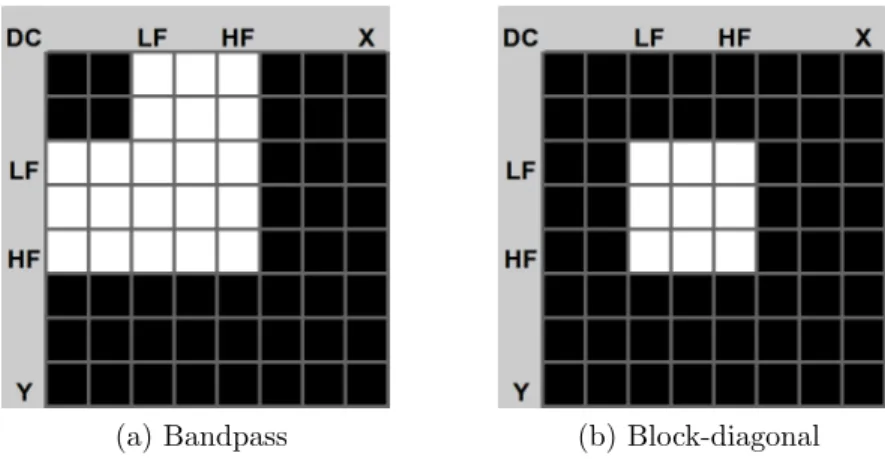
While iterative optimization via gradient or coordinate descent methods is an ob-vious approach for automatic learning, experiments showed that such iterative meth-ods frequently terminate in local minima on the highly-nonlinear cost surface. We propose instead to learn detectors by randomly-sampling frequency coefficient values while varying the size and position of a coefficient mask that zeroes all coefficient values outside of the mask. We refer to our mask of choice as a block-diagonal con-straint, as illustrated in Figure 3.3. We also evaluate the performance of sampling with bandpass constraints and sampling raw pixel values via the na¨ıve approach. In all cases, sampled values are taken from a uniformly-random distribution in the range [-127,127].

(a) Bandpass (b) Block-diagonal

Figure 3.3: Illustrations of frequency-domain filter constraints for 8_×8 filters. Coefficients rendered in black are suppressed (forced to zero). White coefficients may take any value. A typical bandpass filter is shown in (a). We propose the use of the block-diagonal region of support (b), which exhibited superior performance in our tests.

The constraints illustrated in Figure 3.3 are defined by low and high frequency cutoffs, which define the filter’s bandwidth. The filters shown have low and high

(35)

frequency cutoffs of 0.250 and 0.625, respectively2

. Thus, the filters have a bandwidth of 0.375.

Iteratively-optimizing with the target application in the loop can be very expen-sive. Steepest descent methods that use the local gradient of the error function require at least nerror evaluations for square filters of width √n. After gradient calculation, multiple step lengths may be tried in a line-search minimization algorithm. At a minimum, n + 1 error evaluations are required for every update. Coordinate de-scent methods require at least 2n evaluations to update every coefficient once. Both methods require more calculations in practice. Because the error surface contains a high number of local minima, step sizes must be small and optimization converges quickly. This results in a great deal of computation for only small changes to the filter. We found that 95% of our best randomly-sampled filters did not reduce their error significantly after iterative optimization. Many did not improve at all.

In contrast to iterative methods, computing the error for a new filter only requires one evaluation. The result is that in the time it would take to perform one round of gradient descent for an 8_×8 filter, we can evaluate a minimum of 65 random samples.

3.3 Stereo visual odometry

This section details the specific implementation of the stereo visual odometry system used for feature detector learning. In principle, our in-situ training methods apply to other stereo visual odometry pipelines and other applications. Prior work in visual motion estimation demonstrated accurate and reliable, high-frame rate operation us-ing corner feature detectors [7, 5]. A number of system architectures are possible and have been demonstrated in the literature, including monocular [5, 4] and stereo approaches [7, 22].

3.3.1 Visual odometry overview

Our approach to stereo visual odometry can be divided into a number of sequential steps:

1. Image acquisition- 30 Hz hardware-triggered frames are paired using embed-ded frame counters before performing stereo rectification via bilinear interpola-2

(36)

tion

2. Feature detection - Features are detected in grayscale images with non-extrema suppression. Zero-mean, 9_× 9 pixel patch descriptors are used for all features

3. Matching - Features are matched between paired images using a zero-mean Sum of Absolute Differences (SAD) error score. To increase robustness to noise, we search over a +/-1 pixel offset when matching. Unique matches are triangu-lated and added to the map. Previously-mapped features are projected using their last known 3D position and matched locally

4. Outlier rejection- Robustness to incorrect correspondences is provided through both Random Sample Consensus (RANSAC) and “robust” cost functions in the estimator (specifically, the Cauchy cost function withb = 1.0) [46, 8]

5. Motion estimation - The motion estimate is initialized to the best pose es-timated in RANSAC. The point and camera motion estimates are improved through non-linear optimization, iterating until convergence is achieved

The result is an updated 3D feature set and an estimate of the camera motion between the two sequential updates.

3.3.2 Ground truth using AprilTags

We compute our ground truth camera motion by instrumenting the scene with April-Tags and solving a global non-linear optimization over all of the tags and camera positions. Specifically, the four tag corners are treated as point feature detections with unique IDs for global data association. During learning, we explicitly reject any feature detections on top of or within a small window around any fiducial marker so that we do not bias the detector learning process. In other words, our system rejects detections that would otherwise occur due to the presence of AprilTags in the scene and focuses on the use of natural features in the environment. This is illustrated in Figure 3.4b, where red overlays correspond to regions where all feature detections are discarded. By using the reprojected fiducial marker positions, we can reject features on markers even when the marker is not detectable in the current frame.

(37)

(a) Reconstruction of the ground-truth camera tra-jectory and landmark positions

(b) Reprojected ground-truth markers

Figure 3.4: Ground truth camera motion reconstruction using AprilTags. Stereo camera trajectory (orange) in (a) is reconstructed using interest points set on the tag corners de-termined by the tag detection algorithm. Shaded region (blue) corresponds to the scene viewed in (b). The mask overlays (red) in (b) are the result of reprojecting the tag corners using the ground truth reconstruction and are used to ensure that no features are detected on the fiducial markers added to the scene. Example feature detections from the best filter learned in this work are shown for reference (green).

(38)

With the ground truth trajectory known, the accuracy of the visual odometry pipeline can be evaluated for every candidate feature detector. For every sequential pair of poses in the dataset, the 3D positions of the ground truth features (the corners of the fiducial markers) are computed with respect to the first of the two poses. These points are transformed to the reference frame of the second camera pose using the motion estimate from the candidate feature detector. Once transformed, the reprojection error is computed against the set of detections from the second camera image pair. E(w) is the mean reprojection error over all pairs of poses in the dataset using this method. It measures how well, on average, the ground truth features are aligned with their observations when using the candidate detector.

3.4 Experiments

Our experiments focus on randomly-sampling filters under different constraints and computing the mean reprojection error of the visual odometry solution with the se-lected filter. In addition, we compare both error and computation time to existing and widely-used feature detectors.

3.4.1 Implementation details

Training and testing was carried out on four datasets between 23 and 56 seconds in length, recorded at 30 FPS. These datasets were collected in various indoor envi-ronments, including an office, conference room, cubicle, and lobby. In each case, 15 seconds of video were randomly selected for training. Figures 3.4 and 3.6 show cam-era trajectories and imagery from these datasets. This stereo rig included two Point Grey FireFly MV USB 2.0 color cameras at a resolution of 376_×240. Experiments were run on a pair of 12-core 2.5 GHz Intel Xeon servers, each with 32 GB of mem-ory. Sampling 5,000 filters required approximately 7 hours, averaging 9.7 seconds per filter.

In contrast to the substantial computational resources used in learning, our target application is limited to the compute available on a typical mobile robot. A mobile-grade processor such as the OMAP4460, a dual-core ARM Cortex-A9 device, used as an image preprocessing board, is a compelling and scalable computing solution to our needs. With a convolution implementation optimized via vector instructions,

(39)

(a) Office (b) Conference room

(c) Cubicle (d) Lobby

Figure 3.5: Images from the four datasets used for feature detector learning. Masks for AprilTag fiducial markers are shown in red.

(40)

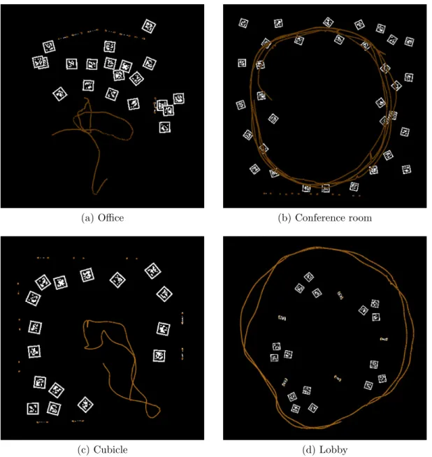
(a) Office (b) Conference room

(c) Cubicle (d) Lobby

Figure 3.6: Reconstruction of the ground-truth camera trajectories and landmark positions. The positions of the AprilTag fiducial markers (black and white textures) and the full camera trajectory (orange line) are jointly estimated to provide ground-truth reference data for training

(41)

specifically ARM NEON, we can detect around 300 features per 376_×240 image in 3.65 ms for a 8_×8 filter. In comparison, the ID3-optimized version of the FAST feature detector performs similarly, requiring 3.20 ms. For both methods, we dynamically adjust the detection threshold to ensure the desired number of features are detected even as the environment changes.

Figure 3.7: Time comparison between FAST-9 and an 8_×8 convolutional filter feature detector. Times represent the combined detection and non-extrema suppression time and were computed on the PandaBoard ES (OMAP 4460) over 30 seconds of video with 376x240, grayscale imagery.

While both methods are efficient enough for real-time use, the difference in com-putation time for a large number of features is dramatic. Figure 3.7 shows the runtime as a function of the desired number of features for both methods. This time measure-ment includes detection and non-extrema suppression. While both methods show a linear growth in computation time, the growth for the convolutional methods is much slower than for FAST. This is because the convolution time does not change as the detection threshold is reduced. The linear growth is due only to non-extrema sup-pression. This result is especially important for methods where the desired number of detections is high [5, 22].

3.4.2 Randomly-sampled filters

The proposed learning method was evaluated through a suite of random-sampling experiments for block-diagonal filters with both the DCT and Haar parameterization. We also compare to sampled bandpass and pixel filters. Figure 3.8 shows the error

(42)

of the best filter sampled so far as 5,000 filters are sampled. In all four datasets, the pixel and bandpass filters never outperformed the best block-diagonal filter. The final filters of each type and from each dataset3

are shown in Figure 3.9.

Figure 3.10 shows the error distributions for each of the three constraints on the conference room dataset. For each experiment, 5,000 filters were randomly generated with the appropriate set of constraints. For the bandpass and block-diagonal con-straints, we generated filters for all combinations of the DCT or Haar transform low frequency cutoff and filter bandwidth, defined previously. Of the 27 combinations of low and high-frequency mask cutoffs available for both DCT and Haar filters of size 8_×8 (in total, 82

−1 combinations each for DCT and Haar), only 6 of them include the DC component and, in the case of the block-diagonal filters, the vertical and horizontal edge components.

From these plots, it is clear that limiting the search for a good filter through the bandpass and block-diagonal sampling constraints significantly improved the percent-age of filters which yield low reprojection errors. Our interpretation of this result is that these filter-based detectors are sensitive to nonzero values for specific frequency components. By strictly removing these components in 21 of the 27 constraint com-binations, the average filter performance improves significantly.

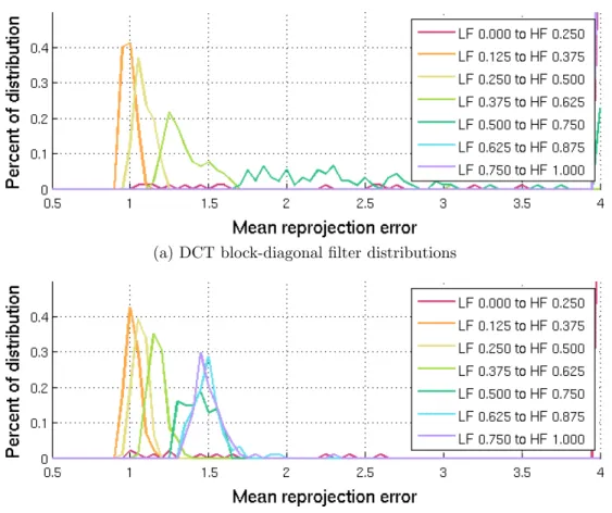
Figure 3.11 shows separate distributions for block-diagonal filters for each of the possible low-frequency cutoffs for filters with the most narrow filter bandwidth (0.250). One plot is shown for each frequency transformation (DCT and Haar). From these figures/filters, it is clear that filters perform significantly worse when the DC and edge coefficient values are not zero. Beyond that, there is a clear trend of low error for low-frequency filters, and an increasing error as frequency increases. Finally, the DCT filter performance significantly degrades as high frequency components are introduced; however, the Haar filter performance does not. Our interpretation of this result is that, because Haar basis patches are not periodic, a simple step transition in an image will often result in a single, unique maxima. In contrast, the periodic DCT basis patches will yield multiple local maxima, causing a cluster of detections around edges. Similar trends exist for filters with higher bandwidths.

The performance of the best sampled block-diagonal filters are compared to base-line methods such as FAST, Shi-Tomasi, a Difference of Gaussians filter, and filters used by Geiger et al. in Table 3.1. The best result from every testing dataset (row)

(43)

(a) Desk dataset (b) Conference room dataset

Figure 3.8: Mean reprojection error for the best convolutional filter sampled so far (running minimum error) over 5,000 samples. Ground truth system error shown in red.

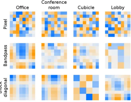
Figure 3.9: Visualization of the best learned convolutional filter for each combination of dataset and sampling type. Best viewed in color.

(44)

(a) Pixels (b) Bandpass (c) Block-diagonal

Figure 3.10: Histogram of mean reprojection errors for three filter generation methods on the conference room dataset. While randomly-generated bandpass filters yield better performance, on average, than filters with uniformly-random pixel values, block-diagonal filters have both better average performance and a lower error for the best filters. 79% and 72% of sampled bandpass and block-diagonal filters, respectively, had errors under 2.5 pixels, while only 30% of random pixel filters had such low errors.

is shown in bold. All detector evaluations were performed with the same system pa-rameters: 300 detected features after non-extrema suppression and rejection due to fiducial marker masks, use of RANSAC and a Cauchy robust cost function (b= 1.0), etc. These parameters were set via parameter sweeps using the FAST feature detector on the office and conference room dataset. As such, these represent best-case con-ditions for FAST. Mean values over 25 trials are reported due to variability induced by RANSAC. The differences in the means between the trained filters and FAST were statistically significant in 10 of the 12 cases with p values less than 0.01 for a two-tailed t-test.

These results reinforce the notion that learned convolutional filters can compete with non-linear detection methods, like the FAST feature detector. Only on the con-ference room dataset did FAST perform better than a learned filter. On average, learned filters had a lower reprojection error than FAST by a small amount, 0.05 pixels. For other baseline methods, such as Shi-Tomasi, the improvement in reprojec-tion error was substantial. Note that while SURF outperformed all methods on the cubicle dataset, this is due to SURF detections adjacent to AprilTags that cannot be rejected in the same manner as other features due to SURF’s scale invariance.

For the linear baseline methods, the results vary greatly. Geiger et al.’s corner filter performs the best of the three, and yet it and the other linear baselines perform

(45)

(a) DCT block-diagonal filter distributions

(b) Haar block-diagonal filter distributions

Figure 3.11: Distributions of block-diagonal filter reprojection errors for filters with a band-width of 0.250 on the conference room dataset. For both (a) and (b), the filters which include the DC and vertical/horizontal edge components (LF cutoff of 0) have reprojection errors greater than 4 pixels 84% and 87% of the time for DCT and Haar filters, respectively. Be-yond the DC components, only the DCT filters with low-frequency cutoff of 0.5 or greater have such large reprojection errors. The remaining distributions progress smoothly from low error (left) to high error (right) as the frequency increases. Best viewed in color.

(46)

Test Set Filters trained on dataset Linear baselines Non-linear baselines Office Conf. rm. Cubicle Lobby DOG Geiger Corner Geiger Blob FAST Shi-Tomasi SURF

Office 0.447 0.466 0.471 0.468 40.281+ _0.492 _0.595 _0.470 _2.060 _1.322∗

Conf. room 0.981 0.929 0.996 0.981 1.505 1.047 1.218 0.953 1.141 1.584∗

Cubicle 1.292 1.142 1.134 1.368 2.962 2.131 4.042 1.441 4.550 0.795∗

Lobby 1.593 1.552 1.628 1.482 1.974 1.573 1.927 1.654 1.938 2.032∗

Table 3.1: Motion estimation testing error (pixels) on each dataset using learned feature detectors and baseline methods. Reported numbers are mean values over 25 trials to com-pensate for the variability of RANSAC, except for the training errors (gray). Bold values are the best result for every row. ∗_{SURF generated features adjacent to AprilTags that}

could not be easily filtered out due to SURF’s scale variation. As such, the SURF results are not considered a fair comparison to the other methods. +

Unusually large mean error is the result of data association failures for the specified feature type

quite poorly on the cubicle dataset, unlike the learned filters. Interestingly, these linear detectors (or an equivalent 8_×8 filter) are simply a few of the convolutional filters that could have been learned in our framework.

These results also suggest that dataset choice, not learned filter, was the best predictor of testing errors. The cubicle dataset had a high error in a number of cases. From inspecting the video stream, this is not surprising — the cubicle is generally feature-deficient except for smooth edges and a narrow strip where the camera sees long-range features over the cubicle wall.

3.5 Summary

Feature detectors are primarily designed manually and evaluated with proxy metrics that aren’t guaranteed to reflect the requirements of a target application. This work addressed this issue by automatically learning feature detectors in a general convolu-tional filter framework. The learned detectors were automatically tuned to maximize the accuracy of the motion estimate computed by a stereo visual odometry pipeline. The resulting detectors outperform a comprehensive set of baselines and yield con-sistent performance on the cubicle dataset, which disproportionally challenged most baseline methods. Additionally, these results demonstrate that the learned features are robust across datasets, as each training dataset produced filters that were similarly or more accurate than the baseline methods when evaluated across testing datasets.

(47)

experimentally determined that gradient and coordinate descent methods quickly converge in local minima without substantial improvement over a filter’s initial per-formance, and we argue that the computation time required to compute a gradient update step is better spent exploring tens, if not hundreds, of random samples. We propose a mechanism to usefully distribute samples throughout the frequency domain by sweeping over block-diagonal coefficient masks. Further, we demonstrate a trend in both DCT and Haar wavelet-based filter performance that favors low-frequency filters.

(48)

Chapter 4 Feature descriptor learning

Feature descriptors generated by a sequence of two-pixel intensity comparisons are capable of representing image features tersely and quickly. These so-called binary

or Boolean string descriptors, which store a comparison’s outcome in a single bit, require only a few bytes per feature (e.g. 8-64B, often 32B), greatly reducing memory footprint and network transfer bandwidth. In addition, computing and matching these descriptors requires much less runtime than well-known alternatives like SIFT and SURF, with comparable matching accuracy [33, 24].

One such method, BRIEF [33], is notable due to its intuitive formulation and compatibility with vector instruction sets. But unlike one of BRIEF’s predecessors, Randomized Trees [59, 60], BRIEF’s comparisons are fixed and do not adapt to the image content of individual image features. This makes BRIEF sensitive to viewpoint change, as the intensities shifting under the fixed sampling pattern can cause the test outcomes, and thus the computed descriptor, to change. This results in increased overlap between descriptor error distributions for true and false correspondences, which ultimately leads to a higher false match rate.

Two of BRIEF’s primary advantages are the small memory footprint and fast runtime. These are suited to the demands of real-time vision applications, with constrained bandwidth and high-FPS runtime targets. However, they also set a high bar for improvements — increases in descriptor robustness must come with minimal side effects. How to do this given the unique formulation of BRIEF — the Boolean string representation and use of XOR_/POPCNT _{— is not especially clear.}

This work proposes a formulation for online descriptor learning that improves the matching performance for BRIEF-like descriptors. This is achieved by addressing the sensitivity of intensity-test descriptors to viewpoint variation between multiple

Learning and Searching Methods for Robust, Real-Time Visual Odometry.