Learning the Structure of Bayesian Networks with Constraint Satisfaction

(1)

University of Massachusetts Amherst

ScholarWorks@UMass Amherst

Open Access Dissertations

2-2010

Learning the Structure of Bayesian Networks with

Constraint Satisfaction

Andrew Scott Fast

University of Massachusetts Amherst, [email protected]

Follow this and additional works at:https://scholarworks.umass.edu/open_access_dissertations Part of theComputer Sciences Commons

This Open Access Dissertation is brought to you for free and open access by ScholarWorks@UMass Amherst. It has been accepted for inclusion in Open Access Dissertations by an authorized administrator of ScholarWorks@UMass Amherst. For more information, please contact

[email protected].

Recommended Citation

Fast, Andrew Scott, "Learning the Structure of Bayesian Networks with Constraint Satisfaction" (2010).Open Access Dissertations. 182.

(2)

LEARNING THE STRUCTURE OF BAYESIAN

NETWORKS WITH CONSTRAINT SATISFACTION

A Dissertation Presented by

ANDREW S. FAST

Submitted to the Graduate School of the

University of Massachusetts Amherst in partial fulfillment of the requirements for the degree of

DOCTOR OF PHILOSOPHY February 2010

(3)

c

Copyright by Andrew S. Fast 2009

(4)

LEARNING THE STRUCTURE OF BAYESIAN

NETWORKS WITH CONSTRAINT SATISFACTION

A Dissertation Presented by

ANDREW S. FAST

Approved as to style and content by:

David Jensen, Chair

Oliver Brock, Member

Victor Lesser, Member

Andrea Foulkes, Member

Andrew G. Barto, Department Chair Department of Computer Science

(5)

(6)

ACKNOWLEDGMENTS

This thesis would not have been possible without the kindness and support of David Jensen and Victor Lesser. Together they are responsible for helping me build the foundation on which this thesis is built. Victor gave me my first chance to try research and I am indebted to him for that opportunity. David, my advisor, has been invaluable to me over the years and his encouragement kept me going through the entire process. For this thesis and my research in general, I have adopted David’s em-pirical sensibilities as my own and I hope that this rich heritage is evident throughout my work. David is truly both a gentleman and a scholar and it is a privilege to be his student.

In addition to David and Victor, I am grateful for many others who contributed time and energy towards my journey. I am especially grateful to my other committee members: Oliver Brock and Andrea Foulkes, who were both extremely helpful in providing focus and identifying the weak spots in my arguments and my results. Michael Hay was instrumental in shaping the early stages of this work and provided a knowledgeable sounding board the rest of the way as well. Jennifer Neville provided a consistent reminder that I alone was responsible for seeing this thesis through, while being willing to help in any way she could. I also thank the past and present members of the Knowledge Discovery Laboratory: Lisa Friedland, Marc Maier, Amy McGovern, Huseyin Oktay, Matthew Rattigan and Brian Taylor for being there along the way and helping sharpen the product that you see here. Cindy Loiselle provided more than her fair share of grammar corrections and this document would be wholly

(7)

Cornell provided expert technical advice at all levels and at nearly every hour of the night and day; I never found a problem they were not able to help me solve.

On a more personal note, Trevor Strohman and Jerod Weinman were only a phone call away when I was ready for a bitter end. Their friendship and encouragement meant a lot over the many rough patches. I am also grateful for Evie and Gram whose prayers and friendship made the last months bearable and warmly welcomed us back to Amherst for my defense. My parents, Loren and Lorraine, helped me foster a curious and scientific mind, laying the ground work for this thesis even from an early age. Finally, this thesis is a product of the continual encouragement and love of my wife Anna and son Peter who helped me to weather the ups and downs of research, and who, through their patience and understanding, helped me see this thesis through to completion.

(8)

ABSTRACT

LEARNING THE STRUCTURE OF BAYESIAN

NETWORKS WITH CONSTRAINT SATISFACTION

FEBRUARY 2010

ANDREW S. FAST

Ph.D., UNIVERSITY OF MASSACHUSETTS AMHERST

Directed by: Professor David Jensen

A Bayesian network is graphical representation of the probabilistic relationships among set of variables and can be used to encode expert knowledge about uncertain domains. The structure of this model represents the set of conditional independencies among the variables in the data. Bayesian networks are widely applicable, having been used to model domains ranging from monitoring patients in an emergency room to predicting the severity of hailstorms. In this thesis, I focus on the problem of learning the structure of Bayesian networks from data. Under certain assumptions, the learned structure of a Bayesian network can represent causal relationships in the data.

Constraint-based algorithms for structure learning are designed to accurately iden-tify the structure of the distribution underlying the data and, therefore, the causal relationships. These algorithms use a series of conditional hypothesis tests to learn independence constraints on the structure of the model. When sample size is lim-ited, these hypothesis tests are prone to errors. I present a comprehensive empirical

(9)

evaluation of constraint-based algorithms and show that existing constraint-based algorithms are prone to many false negative errors in the constraints due to run-ning hypothesis tests with low statistical power. Furthermore, this analysis shows that many statistical solutions fail to reduce the overall errors of constraint-based algorithms.

I show that new algorithms inspired by constraint satisfaction are able to produce significant improvements in structural accuracy. These constraint satisfaction algo-rithms exploit the interaction among the constraints to reduce error. First, I introduce an algorithm based on constraint optimization that is sound in the sample limit, like existing algorithms, but is guaranteed to produce a DAG. This new algorithm learns models with structural accuracy equivalent or better to existing algorithms. Second, I introduce an algorithm based constraint relaxation. Constraint relaxation combines different statistical techniques to identify constraints that are likely to be incorrect, and remove those constraints from consideration. I show that an algorithm combining constraint relaxation with constraint optimization produces Bayesian networks with significantly better structural accuracy when compared to existing structure learning algorithms, demonstrating the effectiveness of constraint satisfaction approaches for learning accurate structure of Bayesian networks.

(10)

LIST OF TABLES

Table Page

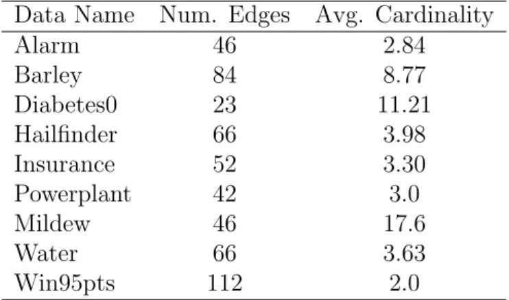
4.1 Number of edges and average cardinality of Bayesian networks

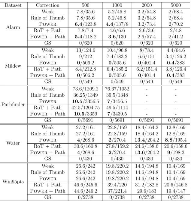
considered during error analysis. . . 28 4.2 The effect size parameters chosen via cross-validation. . . 39 4.3 Corrections for false negative errors. . . 41 4.4 Number of false negative and false positive (fn/fp) errors after

applying corrections to the FAS algorithm. Bold text indicates a significant reduction in false negatives compared to the rule of thumb averaged across 5 training samples. Differences were

significant at the 0.05 level using a one-sided t-test. . . 44

6.1 Likelihood on datasets with unknown structure. Bold indicates a

significant improvement over_Edge-Opt. . . 77 7.1 P-values of the differences in compelled F-measure and structural

Hamming distance (SHD) between_Relax and the baseline

algorithms. Italics indicate thatRelaxhas worse

performance. . . 93

7.2 Proportion of runs on Alarm, Insurance, Powerplant, and

Water whereRelax exceeds the other algorithms on each

metric. . . 94

7.3 Likelihood on datasets with unknown structure. Bold indicates a

significant improvement over_Relax. . . 95 A.1 Summary statistics of Bayesian networks used in this thesis. . . 109

(15)

LIST OF FIGURES

Figure Page

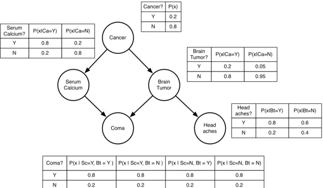
2.1 An example Bayesian network modeling the relationship between

cancer and common symptoms. Probability distributions are

shown in the tables. The example is due to Pearl [74]. . . 6

4.1 A Decision Tree used to determine the composition of the

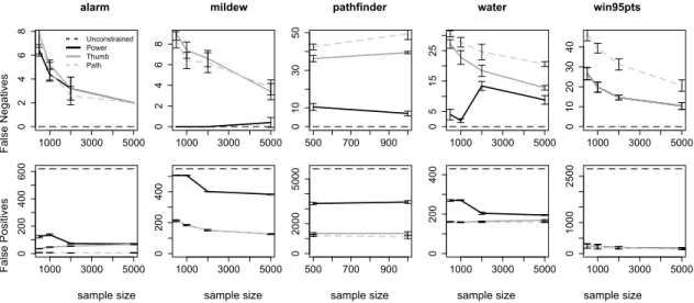
constraints. . . 25 4.2 Number of false negative (FN) and false positive (FP) errors. False

positive errors are decomposed into errors due to making a default decision and due to a statistical error. In all figures, fewer errors

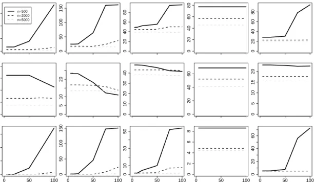
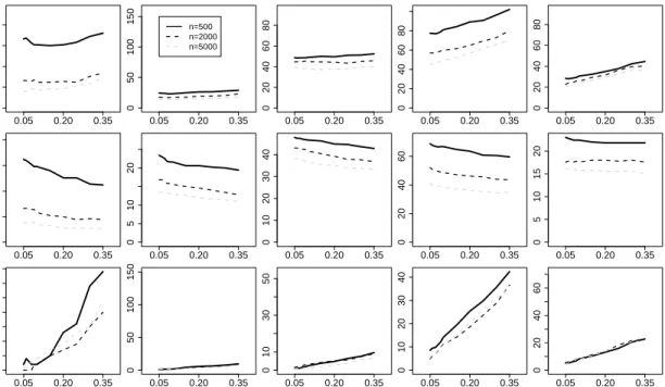
is better. . . 28 4.3 CDFs of true versus learned sepsets. . . 29 4.4 Minimum statistical power permitted under the rule of thumb. . . 35 4.5 Results of cross-validation to select the best effect size parameter.

The dashed grey lines indicate the outer limits considered during cross-validation. The minimum indicates the largest effect size where no tests are run and the maximum indicates the tests that

are run under the rule of thumb threshold. . . 40 4.6 Comparison of the number of false negative and false positive errors

for all the corrections. Error bars indicate 95% confidence

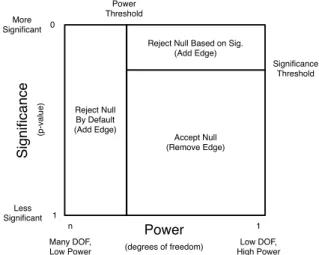
intervals about the mean of 5 runs. . . 42 5.1 Pictorial representation of the two thresholds for determining power

of a hypothesis test. . . 47 5.2 Skeleton errors as DOF threshold increases to improve power . . . 49 5.3 Skeleton errors as significance threshold decreases to improve

power. . . 50 5.4 Skeleton errors made by the FAS algorithm after replacing theχ2 _test

(16)

5.5 Structural accuracy of the different matching approach on marginal

(pairwise) tests. . . 60 5.6 Skeleton errors using propensity score matching with a significance

threshold of p= 0.0001. . . 61 5.7 Skeleton errors using propensity score matching as the significance

threshold varies. . . 62

6.1 Anatomy of a bidirected edge. Since the PC-Edge algorithm

considers constraints independently, overlapping colliders are oriented with a bidirected edge as a result of errors in the

constraints. . . 67 6.2 The Toggle-Collider operator . . . 72

6.3 Comparison of Compelled F-Measure across number of random

restarts for each value of k. . . 74

6.4 Comparison of Compelled F-Measure across values of k for each

number of random restarts. . . 81 6.5 Number of triples in the learned constraints as sample size grows.

The increase in the number of triples can be accounted for by the increase in statistical power as sample increases. . . 82

6.6 Compelled F-measure and structural Hamming distance (SHD) rates

of PC-Edge and Edge-Opt. Differences are significant at

p= 0.01 on Powerplant and Win95ptsnetworks and

statistically indistinguishable in the other cases. . . 82

6.7 Compelled F-measure and structural Hamming distance (SHD) rates

of PC-Edge and Edge-Opton datasets generated using the

BNGenerator package. Differences are significant at p= 0.01 on

both metrics. . . 83

6.8 Runtime of Edge-Optalgorithm with 25 restarts compared with

other algorithms. . . 83

7.1 Evaluation of structural accuracy using compelled F-measure and

structural Hamming distance. . . 93 7.2 Loglikelihood on generated datasets. . . 95 7.3 Runtime of the Relaxalgorithm and the comparison algorithms. . . 96

(17)

7.4 Distribution of the parameters of the true networks. . . 97 7.5 Compelled precision and recall. . . 100

7.6 BDeu results of the learned model computed on a held-out test set of

10000 instances sampled from the true model (higher is

better). . . 100 7.7 Additional edge metrics. . . 101 A.1 Distributions of the cardinality of variables for the ten networks

(18)

CHAPTER 1 INTRODUCTION

A Bayesian network is a directed, acyclic, graphical representation of the prob-abilistic relationships among a group of variables. The network is defined by a set of conditional distributions that can be used to represent the joint probability dis-tribution over the variables. The graphical structure of a Bayesian network model describes, in an understandable, visual manner, which variables have direct influence on other variables under consideration. Consequently, Bayesian networks have long been used to encode expert knowledge about uncertain domains [41].

To augment available expert knowledge, many algorithms have been developed to learn the structure of Bayesian networks from data [16, 18, 25, 44, 85]. When certain assumptions hold, the structure of Bayesian networks has a causal interpre-tation [75, 76, 87]. If the structure of a causal model is accurate, it can be used to predict the effects of manipulations, called interventions, on the system being studied [75]. Consequently, structure learning of Bayesian networks can be used to identify actionable knowledge, which is also the goal of the field of knowledge discovery from databases (KDD) [32, 34].

The focus of this work is developing structure learning algorithms for Bayesian networks that produce actionable models where the structure of the model accurately captures the causal relationships in the data. A subset of structure learning algo-rithms, calledconstraint-based algorithms, are designed for this purpose. [75, 76, 87]. These algorithms operate in two independent phases [18, 87]. The first phase, called

(19)

of independence constraints on the structure of the final model. The second phase, called edge orientation, merges the learned independence constraints into a fully di-rected Bayesian network model. While constraint-based approaches are sound in the sample limit [76, 87], at more reasonable sample sizes typically encountered in prac-tice, the hypothesis tests used to identify the constraints are not perfectly accurate, leading to errors in the learned model structure and incorrect causal conclusions.

The primary innovation of this thesis is the development of new algorithms, in-spired by constraint satisfaction, that are able to learn more accurate structure of Bayesian network than existing constraint-based algorithms. Like traditional straint satisfaction algorithms, but in contrast to constraint-based algorithms, con-straint satisfaction algorithms for learning the structure of Bayesian networks consider all independence constraints jointly. In the remainder of the thesis, I provide addi-tional motivation for this new approach to structure learning and show how constraint satisfaction techniques can produce learned models with significantly fewer structural errors than existing approaches. Chapters 2 and 3 provide background on Bayesian networks and motivate the constraint-based structure learning paradigm. Chapter 4 presents an empirical evaluation of existing constraint-based algorithms that shows false negative errors as the most prevalent error in constraint identification. Further-more, that evaluation demonstrates that the majority of the false negative errors are a result of running low-power hypothesis tests and that the existing methods used for controlling false negative errors are not able to adequately account for all factors contributing to low statistical power. Chapter 5 considers statistical approaches for improving the statistical power of constraint identification, including a new approach based on propensity score matching. The empirical results presented there show that there is a fundamental trade-off between false negative and false positive errors and that it is difficult to achieve gains in power without a significant increase in false

(20)

positive errors. Therefore, alternative approaches are needed for improving the rate of errors.

Constraint satisfaction provides an alternative approach for reducing errors in structure learning. Constraint satisfaction algorithms use the same independence constraints as existing algorithms, but exploit the interaction among the constraints by considering the constraints jointly instead of independently and by using search in place of deterministic rules. Chapter 6 describes the first algorithm to use con-straint satisfaction ideas for structure learning. This algorithm, using a concon-straint satisfaction strategy called constraint optimization, considers all constraints jointly and is guaranteed to produce a Bayesian network, unlike existing edge orientation algorithms. The models learned using constraint optimization meet or exceed the accuracy of the models learned using the previous approach. Constraint optimiza-tion alone is not sufficient to reduce errors as the constraints being satisfied could be incorrect. However, since constraint optimization guarantees that the learned struc-ture is a directed acyclic graph, it enables other constraint satisfaction approaches for structure learning.

Constraint relaxation is a constraint satisfaction approach that allows learned in-dependence constraints to be “relaxed” or corrected in the face of additional evidence. Combined with constraint optimization, constraint relaxation is a powerful way to im-prove the accuracy of learned structure. Chapter 7 describes the first algorithm for constraint relaxation. This algorithm combines multiple structure learning strategies and unifies constraint identification and edge orientation into a single algorithm. The result is an algorithm that produces models with significantly higher structural accu-racy than competing approaches. Implementation of these new constraint satisfaction

algorithms are available in thePowerBayesopen-source software package, which is

(21)

As experimental results throughout the thesis demonstrate, incorporating con-straint satisfaction approaches into algorithms for learning Bayesian networks pro-duces significant reductions in error over previous algorithms. The algorithms intro-duced in this thesis embody two primary strategies for reducing errors in structure learning of Bayesian networks. First, constraint satisfaction permits the reduction in errors by incorporating more available information than existing algorithms during structure learning. The constraint optimization algorithm is the first edge orienta-tion algorithm to consider all independence constraints jointly. Constraint relaxaorienta-tion is the first approach to do model selection based on the constraints and simultane-ously unify constraint identification and edge orientation into a single search process. Second, these approaches reduce errors by relying on the combination of different, but complementary, techniques in both phases of structure learning. Additionally, the constraint satisfaction approaches introduced in this thesis provide an extensible platform that can incorporate additional advances as they are discovered.

(22)

CHAPTER 2 BACKGROUND

2.1 Bayesian Networks

Bayesian networks are a concise, graphical representation of a joint probability distribution P over a set of variables V. A Bayesian network M = {G,Θ} consists of an acyclic, directed graph G = {V, E} containing vertices and edges and a set

of conditional probability distributions, Θ. The edges of G indicate a dependency

between the variables. Throughout this thesis, I will refer to the collection of edges

in G as the structure of the Bayesian network. The parents of a variable v ∈ V,

denoted pa(v), are the set of variables that are the source of directed edges pointing to the variable v. The children of a variable are all the nodes that are pointed to by edges leaving a variablev, denotedc(v). The neighbors or adjacent variables of a variablev areAdj(v) = pa(v)∪c(v). For each variable,θv is a conditional probability distribution defined as the probability P(v|pa(v)). A Bayesian network is compatible

with a distribution P if P can be factored according to the parent relations defined by the structure of G[75]. An example of a Bayesian network is shown in Figure 2.1 The structure of a Bayesian network also represents the conditional independence relations among the variables. The correspondence between conditional independence relations and certain graphical structures is summarized by thed-separation criterion.

Definition 1. (from Pearl [75]) A path p is said to be d-separated or (blocked) by a set of nodes Z if and only if

(23)

Figure 2.1: An example Bayesian network modeling the relationship between cancer and common symptoms. Probability distributions are shown in the tables. The example is due to Pearl [74].

1. p contains a chain i→m→j or a fork i←m →j such that the middle node m is in Z, or

2. p contains an inverted fork (or collider) i→ m←j such that the middle node m is not in Z and such that no descendent of m is in Z.

A set Z is said to d-separate X from Y if and only if Z blocks every path from a node in X to a node in Y. The definition of d-separation matches an intuitive causal understanding of the edges in the graph.

Pearl [74] gives an alternative, but equivalent, definition of a Bayesian network in

terms of d-separation and a dependency model M. A dependency model is a set of

assertions of the form (X ⊥⊥Y|Z) indicating that “X is independent ofY given Z.”

(24)

M corresponds to a valid d-separation relationship inD; that is, the global structure of D is consistent with every local assertion in M.

2.2 Overview of Structure Learning

Given a set of variablesV and a datasetDcontaining independent and identically

distributed (i.i.d.) instances sampled from an unknown distribution P the goal of

structure learning is to identify a graph G that is compatible with P. To form a

complete modelM, an additional step of parameter estimation is needed to determine

Θ from D. Techniques for parameter estimation are generally well-known and will

not be addressed here (see e.g., Heckerman [41] for more details).

The two definitions of Bayesian networks described in Section 2.1 have led to the development of two broad classes of structure learning algorithms. The first approach, calledsearch-and-score, searches over possible Bayesian network structures to find the best factorization of the joint distribution implied by the training data [16, 25, 44]. The model selection criterion is usually a penalized likelihood score such as BIC [81], AIC [5], or BDeu [15, 44]. The second approach, constraint-based algorithms, learns the structure of a Bayesian network by first running local hypothesis tests

to identify a dependency model M containing independence assertions that hold in

the training data [18, 75, 87, 96]. The learned independence assertions in M are

viewed as constraints on the final model structure, and constraint-based algorithms select a model structure that is consistent with those constraints. A third class of algorithms, called hybrid algorithms, combines techniques from both constraint-based and search-and-score techniques [2, 96].

The different categories of algorithms were each designed with a particular pur-pose in mind. Search-and-score techniques are generally very flexible and find high-likelihood structures but do not enforce conditional independence relationships and often do not accurately reproduce the generating structure [1, 92]. By constraining

(25)

the space with conditional independence relations, constraint-based techniques are more efficient and more accurately recover the structure of the generating distribu-tion but often do not achieve comparable likelihoods with search-and-score techniques [96]. Unlike traditional search-and-score algorithms, constraint-based algorithms ex-ist that have been proven to be sound and complete in the sample limit. Hybrid approaches are designed to take advantage of the power of a constraint-based algo-rithm but while maintaining the flexibility of a search-and-score algoalgo-rithm [96].

No matter which approach is taken, finding an optimal structure for a given set of training data is a computationally intractable problem. Structure learning algorithms determine for every possible edge in the network whether to include the edge in the final network and which direction to orient the edge. The number of possible graph structures grows exponentially with |V|as every possible subset of edges could represent the final model. Due to this exponential growth in graph structures, even a restricted form of structure learning where variables are constrained to have only

k parents has been proven to be NP-Complete [22]. Unless P = NP, there is no

known efficient, polynomial-time algorithm for exhaustively searching the space of possible graph structures to determine a graphical structure that best describes the available data, D. Since an exhaustive search algorithm is not possible, existing structure learning algorithms either solve a restricted problem (i.e., find the best structure given a partial ordering of the variables) or find an approximation to the best compatible graph.

In general, the set of conditional independence relations ofP do not entail a unique

graph structure; there may be many graphs that are compatible with P. Therefore,

accurately identifying conditional independence relationships present in the data may not be sufficient to produce a fully oriented model [19, 21, 87]. Rather than learning a fully directed model, many algorithms instead produce a partially directed acyclic graph (PDAG) model, also called a pattern oressential graph [6, 87, 98]. Edges that

(26)

are directed in the PDAG are edges that are directed in the set of all graphsGthat are

compatible with P. Consequently, edges directed in the PDAG are called compelled

edges as only that edge orientation is compatible with the data [20]. Undirected edges in the PDAG represent edges that could be oriented in either direction and still be compatible with the training data. The set of directed graphs that match a fully directed instantiation of a PDAG are considered to be in the sameequivalence class.

2.3 Evaluating Structural Accuracy

For evaluation purposes, structural accuracy of learned networks can be measured with a variety of different metrics that compare the structure of both the learned and true models. This requires the structure of the true model to be knowna priori. This is typically achieved by generating data from a known model and then learning from that data. The first metric is the accuracy (percent of edges correct) of edges in the model [8, 14, 86]. A closely related metric is the precision and recall of causal struc-tures [60]. I use precision and recall of compelled edges, where compelled precision is defined as the number of correct compelled edges divided by the total number of compelled edges in the learned model. A compelled edge is an edge that has the same orientation in every member of the equivalence class of the learned model [20]. For simplicity, I report a single number, the compelled F-measure, which is the harmonic mean of compelled precision and compelled recall [26] and is a general purpose metric of the correctness and actionability of the structure.

An alternative metric is structural Hamming distance (SHD), based on the raw counts of errors in the learned model [96]. The SHD of a model is a type of graph edit distance and is equal to the number of edge deviations between the model and the true model. It is often expedient to consider decompositions of the SHD, particularly into skeleton errors (false positive and false negative errors) and orientation errors

(27)

(errors of edge direction). I also use the number of true positive edges (number of correct edges) for evaluation.

(28)

CHAPTER 3 CONSTRAINT-BASED ALGORITHMS FOR LEARNING

BAYESIAN NETWORKS

In this thesis, I focus on constraint-based approaches for learning the structure of Bayesian networks from data. Existing constraint-based algorithms perform structure learning in two independent phases. First, using a collection of conditional hypothesis tests, constraint-based algorithms learn independence constraints for variables that can be shown to be conditionally independent in the training data. This is the con-straint identification phase, sometimes called skeleton identification after a popular representation of the constraints as an undirected skeleton, indicating the location but not orientation of edges appearing in the final model. Second, constraint-based algorithms select a fully oriented model using the learned constraints. This phase is often called edge orientation, as it can be viewed as finding an orientation for the undirected edges appearing in the skeleton. In the remainder of the chapter, I provide motivation for choosing a constraint-based algorithm over a search-and-score algorithm and provide greater detail of the inner workings of constraint-based, hybrid and refinement algorithms for learning the structure of Bayesian networks.

3.1 Motivation

One of the motivations for this thesis is to make structure learning of Bayesian networks a better tool for knowledge discovery tasks. Since the goal of knowledge discovery is actionable knowledge, learning accurate structure of the underlying distri-bution is desired. Learning a model that only provides accurate probability estimates,

(29)

but not accurate structure, is not sufficient for taking action because adjusting the variables to change the probabilities might not correspond to adjustments changing the underlying process. Constraint-based algorithms are ideally suited for knowledge discovery tasks for two reasons: (1) they are optimized for producing more accurate structure, and (2) they can produce Bayesian network models with causal interpre-tation in certain situations.

Constraint-based algorithms are better suited for learning accurate structure of Bayesian networks than search-and-score algorithms, which typically use a penalized likelihood score such as BDeu to choose model structures. Since training data are limited, the structure of the true model often contains more parameters than are

supported by the data when optimizing for penalized likelihood. Optimizing for

constraint satisfaction makes it possible to find structures with a large number of parameters as the size of the model is not part of the model selection criterion. In addition, algorithms based on constraints have been proven sound in the sample limit [87].

In addition to being able to learn more accurate structures compared to search-and-score algorithms, constraint-based algorithms can learn Bayesian networks with a causal interpretation when certain assumptions hold about the data [75, 87]. These assumptions are that all variables are measured (no latent variables), the distribu-tion underlying the training data can be represented by a DAG, and the statistical decisions made from the data are correct (e.g., made in the sample limit). I will not focus on these assumptions in this thesis as they cannot be validated experimentally [80]. Rather than seek out expert validation for each dataset under consideration, I will focus on the structure learning component of the causal inference problem. The ability of a structure learning algorithm to recover the generating distribution can be evaluated experimentally if the data are generated from a known model. By

(30)

improv-ing the recovery of the generatimprov-ing structure, it is possible to improve the strength of causal inferences if the assumptions above are valid for a given data set.

3.2 Constraint Identification

Constraint-based algorithms are based on Pearl’s definition of a Bayesian network

in terms of a dependency model M. Viewed this way, the independence assertions

contained in M are constraints that are learned from data. These assertions are

of the form (X ⊥⊥ Y|Z) indicating that “X is independent of Y given Z.” Each independence constraint is typically decomposed into two parts. The first indicates

a binary decision indicating whether an edge should exist between X and Y. There

is a single constraint for each distinct pair of variables. The collection of all the binary decisions can be represented as an undirected skeleton. The second part of the independence constraints is the separating sets, or sepsets, Z. For each pair of variablesX andY that are determined to be independent, the separating sets indicate which set of variablesZ that are necessary and sufficient to d-separateX fromY.

Constraint identification is the process of learning the skeleton and separating sets from the training data. Due to limited size of the training data, this process is inherently error-prone. The goal of constraint identification is to efficiently identify the independence assertions while minimizing the number of constraints that are inaccurate. Constraint identification algorithms appearing in the literature can be differentiated by three different design decisions: (1) the type of independence test used, (2) the ordering heuristic and other algorithmic decisions, and (3) the technique used to determine the reliability of the the test. The following sections identify the possible choices for each decision and the implications of those decisions on the error rate of the overall algorithm.

(31)

3.2.1 Hypothesis Tests of Independence

Constraint-based skeleton algorithms utilize tests of conditional independence to determine which structure to include in the skeleton. In practice, many types of hypothesis tests are used to determine independence, including classical, Bayesian, and information theoretic tests. Each type of test follows the traditional hypothesis testing framework consisting of null and alternative hypothesis and a significance threshold to determine whether to accept or reject the alternative hypothesis. Since the overall goal of this work is learning accurate constraints, one critical characteristic of hypothesis tests for structure learning is the ability to characterize and bound the rate of errors incurred by running the hypothesis test.

Classical hypothesis tests for categorical data typically utilize either the χ2 _or G2 _{statistic when determining whether to accept the alternative hypothesis [87, 96].}

Both the χ2 _and _G2 _{statistics are computed from a contingency table containing}

counts of variable values occurring in the data. The null hypothesis assumes the data

are independent and distributed as χ2 with degrees of freedom that depend on the

size of the table. The alternative hypothesis is accepted and dependence is proven when the the probability of the observed statistic under the null hypothesis is below a specified significance threshold, typically p = 0.05. The degrees of freedom are an indicator of the number of parameters that can be varied in the model. Fewer parameters indicates more data can be used to estimate each parameter, leading to more accurate estimates. The χ2 distribution can also be used to specify a precise alternative hypothesis for computing statistical power.

An alternative to the classical tests is a hypothesis test based on a Bayesian score such as BDeu [1, 27]. This score is computed for the current network with and without the current edge. If the score is greater for the network with the edge, then the two variables are dependent and the edge is added to the network. One advantage of determining independence with a Bayesian approach is the ability to smooth with a

(32)

prior [27]. Incorporating a prior can mitigate problems with false negative errors due to small sample sizes. Calculation of the false negative rate (i.e., statistical power) during learning with a Bayesian score is difficult; however, as the statistic depends on the number of parameters of the model which vary with the structure being learned. A third approach for testing conditional independence utilizes a test of mutual information [18]. If one variable provides some information about another variable, then the two variables are be dependent. As with all tests of conditional independence, determining mutual information is often noisy at small sample sizes. To address this problem, a threshold is used to determine if the observed effect is significant. Unfortunately, the threshold of significance varies with both sample size and the size of the test [18, 96]. Cheng et al. [18] devised a heuristic approach for choosing a threshold for a given sample. Because a heuristic technique is used and the threshold can vary with sample size, it is difficult to compute a consistent rejection region necessary for performing analysis of statistical power. Though the threshold is designed as a control for statistical power, the threshold is not sufficient for computing power exactly. In addition, Hutter [47] shows that point estimates of mutual information are often inaccurate and that consideration of the second-order distribution is necessary to improve structural accuracy.

In this thesis, I will only consider classical hypothesis tests using the χ2 _score. These tests have a well-defined framework for evaluating the rates of type I and type II error rates. As I will demonstrate in Chapter 4, precise analysis of type I and type II error rates is useful for understanding structure learning algorithms for Bayesian networks.

3.2.2 Ordering Heuristics

Given a particular independence test, each constraint identification algorithm ap-plies the tests in a particular order. Many ordering heuristics appear in the literature;

(33)

instead of presenting each one in detail, I highlight the major categories of ordering heuristics with citations to relevant work.

The predominant type of skeleton heuristics are local algorithms that consider each test independently of other decisions. I use the first and most widely used ordering algorithm: Fast Adjacency Search (FAS). The FAS algorithm for constraint

identification is drawn from steps A and B of the PC 1 algorithm, as described in

Spirtes et al. [87]. Pseudocode for FAS is shown in Algorithm 1. An implementation

of the FAS algorithm can be found in the TETRAD IV2 _{package. FAS operates in}

a breadth-first manner considering all pairwise tests followed by all tests conditioned on a single variable and so on until no more tests can be run.

Other ordering heuristics have been presented in the literature as improvements on the FAS algorithms. Max-Min Parents Childen (MMPC) [95, 96] is the constraint identification algorithm used with the Max-Min Hill Climbing (MMHC) algorithm. FAS and MMPC utilize different heuristics to produce a skeleton with the fewest statistical tests. Abellan et al. [1] propose an additional optimization to FAS that breaks triangles in the skeleton by removing the weakest link among three edges

in the triangle before moving on to the next stage. MMPC operates in a more

depth-first manner, considering all tests for a single target variable before considering additional variables. In a different approach, Xie and Geng [99] describe a recursive splitting algorithm to limit the number of other variables considered when searching for a separating variable. These algorithms share the same asymptotic properties of FAS, but these algorithms either encode additional assumptions from FAS or are not compatible with existing corrections for errors.

1 _{PC is named for its creators Peter (Spirtes) and Clark (Glymour)} 2_{http://www.phil.cmu.edu/projects/tetrad/}

(34)

Neighborhood models are another type of ordering heuristic that considers inter-mediate path information when determining whether to add an edge between the two variables under consideration. If a possible conditioning variable does not lie on a path between the two variables being tested then it should not be used to prove conditional independence. This arises out of the definition of d-separation in graph-ical models (see Section 2.1)[74]. Three-Phase Dependency Analysis (TPDA) is the most prominent neighborhood structure learning algorithm [18]. Steck and Tresp [89] also incorporate neighborhood information into the PC algorithm using an additional constraint, called the Necessary Path Constraint, on the conditioning set of a test.

The FAS algorithm is the oldest and most widely studied constraint identification algorithm [1, 57, 87, 89, 97]. Like MMPC and TPDA, the FAS skeleton algorithm is asymptotically correct. However, unlike the other algorithms, the FAS algorithm is an extensible platform that can incorporate the majority of the other improvements and corrections proposed in the literature. Since one contribution of this thesis is evaluating the efficacy of these innovations, the majority of the reported experiments are run using the FAS algorithm to provide a stable comparison.

3.2.3 Determining the Reliability of a Hypothesis Test

It has long been noted in the constraint-based structure learning literature that the reliability of the hypothesis test used in structure learning is inversely related to the size of the conditioning set; as conditioning sets grow, reliability decreases [27, 87, 96, 97, 100]. There are two distinct but related characteristics of a test that determine its reliability. First, a reliable test meets the distributional assumptions of the statistic used; for example, classical tests assume that the data are asymptotically distributed as χ2 _{. Second, a reliable test has sufficient statistical power. Statistical} power is the probability of successfully identifying a significant effect if one exists in the data. As the size of the contingency table grows, for a fixed amount of data

(35)

both the distributional correspondence and the statistical power decrease, leading to a corresponding decrease in reliability.

Many structure learning approaches utilize a “rule of thumb” to determine whether the distributional assumptions hold and a hypothesis test will be reliable [87, 96]. This rule of thumb states that a test is reliable if there are five or more instances per parameter of the test (degree of freedom) [33]. Other algorithms are designed to limit the size of the possible conditioning sets to improve reliability [36, 97]. This is also one of the arguments for considering neighborhood information when making a statistical decision as neighborhood algorithms use smaller conditioning sets, which improves power [18, 89](see Section 3.2.2). Another approach for improving reliability is to average over multiple models with different structures either with a Bayesian approach [13] or by exploring the inconsistencies encoded in the skeleton [89]. Our focus for this work is knowledge discovery; therefore, I focus on algorithms that produce a single model for easier human interpretation.

If a test is determined to be unreliable, then many algorithms make a default decision to include the edge in the model. When a test is unreliable, an insignificant result does not differentiate between an error and a lack of correlation. The default decision is a decision to automatically reject the null hypothesis and assume depen-dence, providing protection against false negative errors that might occur as a result of unreliable tests.

Accurately determining the reliability of the hypothesis tests is critical for min-imizing errors in the learned constraints. In Chapter 4, I compare the strategies mentioned here with a new approach based on statistical power analysis to determine which approach is most accurate in practice.

(36)

3.3 Alternative Skeleton Algorithms

In addition to constraint-based skeleton algorithms, which use hypothesis tests of conditional independence, there are a variety of alternative approaches for constrain-ing search. Frequent item sets have been used in place of conditional independence tests as a basis for skeleton identification [39]. The Sparse Candidate (SC) algo-rithm uses an iterative search process to determine the best structure subject to the

constraint that no variable can have more than k parents [36]. The parameter k is

determined by the user prior to running the algorithm and can exclude high-scoring structures if set inappropriately. Tsamardinos et al. [96] show that MMHC is a sound and complete version of Sparse Candidate and only requires a single iteration.

In general, any approach for learning the structure of undirected networks could be used as a skeleton formation algorithm e.g., Bromberg and Margaritis [13]. Also, since dependency networks have undirected conditional independence semantics [42], it would be possible to extract an undirected skeleton from a learned dependency network. (Note this approach differs from Hulten et al. [46], which uses a dependency network as a mechanism for caching statistics for Bayesian network learning.)

Many of the early algorithms for learning the structure of Bayesian networks, such as K2, constrained search by requiring the user to specify an ordering over the vari-ables [25]. This is a type of hybrid algorithm where the skeleton is specified by the user. Recent work by Teyssier and Koller describe an algorithm that searches over possible orderings [92]. While this approach is not an algorithm based on indepen-dence constraints, it uses ordering constraints to make search more efficient.

These algorithms do not use conditional hypothesis tests to determine the con-straints. The errors of conditional hypothesis tests are well-defined and have been studied extensively. Since the goal of this thesis is reducing errors in constraint identification, my focus on constraint identification algorithms that use conditional hypothesis tests, though improving these other approaches may also be possible.

(37)

3.4 Constraint-Based Edge Orientation

The PC algorithm is a constraint-based algorithm that utilizes three deterministic edge orientation rules for determining edge direction [18, 76, 87]. These rules are based on the structure between variables and conditioning sets determined during the skeleton phase and are appropriate when all possible causes are represented in the data.

The edge orientation rules are as follows (from Spirtes, Glymour, and Scheines [87, Section 5.4.2]):

1. For each triple of vertices X, Y, Z such that the pairX, Y and the pairY, Z are

each adjacent in the skeleton but X, Z are not adjacent, orient X −Y −Z as

X →Y ←Z if and only ifY is not in the conditioning set separatingX and Z

2. If A → B, B and C are adjacent, A and C are not adjacent, and there is no

arrowhead at B, then orient B−C asB →C.

3. If there is a directed path from A to B, and an edge between A and B, then

orient A−B as A→B.

An alternative formulation of these rules is provided by Meek [65]. The rules are applied in lexicographic order and are proven to be correct in the sample limit when the skeleton and conditioning sets are correct. In most instances, however, the skeleton algorithm will not produce the correct skeleton and conditioning sets. Therefore, empirical analysis is necessary to understand when and how errors during the skeleton phase impact edge orientation.

3.5 Hybrid Learning Algorithms

Hybrid algorithms combine aspects of both constraint-based and search-and-score algorithms. The standard hybrid approach first runs some form of constraint identi-fication followed by a heuristic search limited to the edges appearing in the skeleton

(38)

[96, 97]. Any heuristic search technique for Bayesian network structure learning that can be constrained to the skeleton can be used. These approaches do not use the constraints for model selection.

Heuristic search techniques are the most popular form of unconstrained structure learning algorithms for Bayesian networks. These techniques frame structure learning as a global optimization problem searching for the model structure which optimizes some global score. Popular scores include BIC [81], AIC [5], and BDeu [15, 44]. At each step in the algorithm, all possible edge additions, deletions and reversals are considered. The highest scoring operator is applied to the network and the algorithm continues until no operator can improve the score. Often techniques such as random restarts or tabu lists are maintained to avoid local extrema. These search techniques can be tailored for either generative or discriminative purposes [40].

Rather than searching over all possible model structures, some approaches only search the space of equivalence classes of models [3, 20]. These algorithms consider a smaller search space but do not restrict the possible models within that search space. Other approaches for improving the search phase include advance search operators to escape local extrema [67] and more advanced stochastic search techniques [45].

By combining the strengths of both constraint-based and search-and-score algo-rithm, hybrid algorithms are able to provide many of the advantages of both

ap-proaches. Consequently, a hybrid strategy is instrumental for the success of the

constraint satisfaction approaches introduced later in the thesis.

3.6 Refinement Algorithms

In addition to constraint-based and hybrid approaches, there are refinement ap-proaches for learning the structure of Bayesian networks. A refinement algorithm first runs a constraint-based algorithm (constraint identification and edge orientation) to completion and then uses a complementary approach to improve the final structure.

(39)

Abellan et al. [1] describe a hybrid refinement algorithm. After the PC algorithm has completed, Abellan et al. use heuristic optimization techniques to improve the likelihood of the final models at the expense of the causal interpretation of the models [1]. Bromberg and Margaritis [14] use the logic of argumentation combined with the axioms of conditional probability to refine the results of the PC algorithm based on the logical consistency of the constraints. Refinement algorithms also provide a strong influence on the constraint satisfaction algorithms introduced later in the thesis.

3.7 Summary

Constraint-based algorithms are designed to learn accurate Bayesian network structure from data. Existing constraint-based algorithms, such as PC and TPDA, have been proven to be sound and complete in the sample limit. With more rea-sonable sample sizes, however, these algorithms are prone to errors. Many different approaches have been tried to reduce errors. In the following chapters, I explore many of these approaches and propose new constraint satisfaction approaches to re-duce errors. For these experiments, I primarily use the FAS constraint identification algorithm and the deterministic edge orientation rules as a comparison. Although there many possible choices for each component of constraint-based algorithms, the goal is provide a fair comparison of any new approaches.

(40)

Algorithm 1 Fast Adjacency Search (FAS)

procedure FAS(DataD, Variables V)

P =∅ . P contains dependent pairs of variables

C = Empty graph overV

for v1, v2 ∈V do

P =P ∪ {hv1, v2i} . Assume every pair is dependent, add to P

Add edge hv1, v2i to C .Form complete undirected graph over V

end for

n= 0 . n indicates the size of the candidate conditioning sets.

while |P|>0 do for hv1, v2i ∈P do

RunTest =f alse

adj = Adjacencies(C,v1)\ v2 . Get the neighbors ofv1 excludingv2

if |adj|< n then . No more tests to be run.

P =P\{hv1, v2i} . Remove pair hv1, v2i from P

end if

for S ⊆adj s.t. |S|=n do if Test is not reliable then

Continue

end if

RunTest =true

pV al = Run hypothesis test (v1, v2, S, D) . Run Hypothesis Test.

if pV al > 0.05 then . 0.05 is standard threshold

Add constraint (v1 ⊥⊥v2|S)

Remove edge between v1 and v2 in C

P =P\{hv1, v2i} . Remove pair hv1, v2i from P

end if end for

if RunTest = false then . Insufficient power to run any test.

P =P\{hv1, v2i} end if end for n =n+ 1 end while end procedure

(41)

CHAPTER 4 ERRORS OF CONSTRAINT IDENTIFICATION

The first step in reducing the errors of constraint-based structure learning is un-derstanding the sources of errors. In this chapter, I identify the types and analyze the sources of errors made by the FAS algorithm during constraint identification. The results of this analysis indicate that false negative errors due to low power statistical tests are the largest source of errors during constraint identification.

4.1 Introduction

There are two kinds of errors made during constraint identification: skeleton errors and separating set errors. Recall that the constraints considered here are indepen-dence constraints of the form (X ⊥⊥ Y|Z) indicating that “X is independent of Y given Z,” and there is a single constraint for each unique pair of variables occurring in the network. Skeleton errors are errors in the binary edge decision for a pair of variables, that is, whether to add an edge in the model between those two variables. An error of including an edge in the learned model that does not occur in the true model is afalse positive error. An error of excluding an edge from the learned model that does occur in the true model is a false negative error. Separating set errors, also calledsepset errors, occur when the constraint correctly indicates independence for a pair of variables, but identifies a separating set Z that is not consistent with the true model.

Errors can arise from either the determination of test reliability or the statistical test used by the algorithm for constraint identification. The ordering heuristic, while

(42)

a significant portion of a constraint identification algorithm, cannot directly produce errors. Existing ordering heuristics, including FAS, MMPC, and TPDA, are proven to be correct when the hypothesis tests are perfectly correct (i.e., in the sample limit) [18, 87, 96]. Therefore, the errors occur as a result of a faulty statistical decision, either independently or in conjunction with a faulty decision to run an unreliable test, although there is the potential for complex interactions between the algorithmic and statistical components of constraint identification.

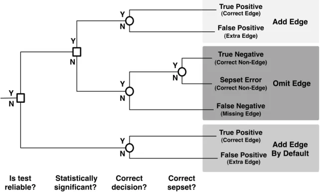
Y N Y N Y N Y N Y N Is test reliable? Statistically significant? Correct decision? True Positive (Correct Edge) False Positive (Extra Edge) True Negative (Correct Non-Edge) False Negative (Missing Edge) True Positive (Correct Edge) False Positive (Extra Edge) Correct sepset? Y N _{Sepset Error} (Correct Non-Edge) Add Edge Omit Edge Add Edge By Default

Figure 4.1: A Decision Tree used to determine the composition of the constraints.

False positive and false negative errors are closely related to traditional type I and type II errors from the statistical literature. Recall that a type I error is the error of rejecting the null hypothesis when it is true, and a type II error is the error of accepting the null hypothesis when it is false. For clarity, I will always refer to false positive and false negative errors in the learned model, while type I and type II errors refer to the results of individual hypothesis tests. Therefore, false positive and false

(43)

negative errors can occur as a result of multiple interacting individual tests, whereas type I and type II errors can only result from a single test. A false positive error in the learned model can occur from either a type I error in an individual test, or as a result of a default decision to add an edge when an individual hypothesis test is determined to be unreliable. A false negative error always occurs as a result of a type II error somewhere in the series of tests leading to the decision to not add the edge to the model. A graphical representation of this decision process is shown in Figure 4.1.

4.2 Analysis of Errors

The frequency of each kind of structural error can be determined by comparing the structure of the learned model with the structure of the model that generated the training data. The easiest way to accomplish this type of evaluation is to gener-ate the training data from a known Bayesian network. A Bayesian network can be created manually by experts or sampled randomly from the space of possible models. Generating data from known models makes possible the evaluation of a learning algo-rithm across a range of sample sizes and data characteristics. It may also be possible to create a biased sampling procedure to synthetically generate models with desired structural characteristics [48].

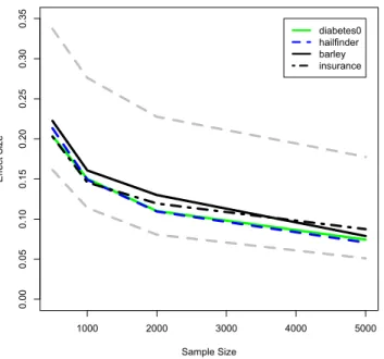
The remainder of this section describes an empirical analysis of the Fast Adjacency Search (FAS) algorithm. The goal of this analysis is to determine whether false positive or false negative errors more frequently occur in runs of the FAS algorithm under realistic conditions. For this exploratory phase of the thesis, I considered datasets generated from eight Bayesian network models gathered from real decision support problems. The list of networks considered along with information about the number of edges appearing in the model and the average cardinality of the variables

(44)

can be found in Table 4.1. Additional details about each of these models can be found in Appendix A.

For each model, I generated five datasets at each of the following sample sizes: n={500,1000,2000,5000,10000}. For each dataset of each model, I ran an annotated version of the FAS algorithm that has access to the true model and, for each edge decision, reports whether that decision results in a statistical false positive, false positive as a result of the default decision (default false positive), or a false negative error. The results of that experiment are shown in Figure 4.2. On every network

with the exception of _Hailfinder, the number of false negative errors dominates

the statistical false positive errors. On networks with low-cardinality variables such

asAlarm, false negative errors also dominate the default false positives as very few

tests have sufficiently large degrees of freedom to trigger the default decision. On

Barley, Diabetes0, and Hailfinder, the default false positives are the largest

source of error at smaller sample sizes but drop below the false negatives at high sample sizes.

The aim of making a default decision is to reduce the overall number of errors, however making the decision to add an edge when the test is unreliable actually leads to more errors than it corrects. The total number of edges appearing in each network is shown in Table 4.1. At the smaller sample sizes, the number of default false positive errors is considerably larger than the total number of edges in the generating model Therefore, a simple way to reduce errors would be to simply run every test and never make a default decision to add an edge. Since the default decision was intended to decrease the chance of making a false negative error, never making a default decision should increase the number of false negative errors.

Additional evidence for the importance of correcting false negative errors is pro-vided by analyzing the separating sets of the learned and true networks. A separating

(45)

Figure 4.2: Number of false negative (FN) and false positive (FP) errors. False positive errors are decomposed into errors due to making a default decision and due to a statistical error. In all figures, fewer errors is better.

alarm 0 10 20 30 40 50 0 5000 10000 Num. Errors FN FP(stat) FP(default) barley 0 40 80 120 0 5000 10000 Num. Errors diabetes0 0 40 80 120 0 5000 10000 Num. Errors hailfinder 0 10 20 30 40 50 0 5000 10000 Num. Errors insurance 0 10 20 30 40 50 0 5000 10000 Num. Errors powerplant 0 10 20 30 40 50 0 5000 10000 Num. Errors water 0 10 20 30 40 50 0 5000 10000 Num. Errors win95pts 0 20 40 60 0 5000 10000 Num. Errors

Table 4.1: Number of edges and average cardinality of Bayesian networks considered during error analysis.

Data Name Num. Edges Avg. Cardinality

Alarm 46 2.84 Barley 84 8.77 Diabetes0 23 11.21 Hailfinder 66 3.98 Insurance 52 3.30 Powerplant 42 3.0 Mildew 46 17.6 Water 66 3.63 Win95pts 112 2.0

(46)

set error occurs when the algorithm concludes independence with a separating set that is not compatible with the true network. For a given pair of variables, there may be multiple separating sets of the minimal size that are all sufficient to d-separate the variables. A learned separating set is compatible with the true network if it is also the minimal size and exactly matches ones of the true separating sets. Since the binary edge decision of independence is correct, separating set errors are the result of what Mosteller [68] has called type III errors—making the right decision for the wrong reason. 0 1 2 3 4 5 0.0 0.4 0.8 alarm

Size of Separating Set

Percentage TrueLearned

0 1 2 3 4 5

0.0

0.4

0.8

insurance

0 1 2 3 4 5

0.0

0.4

0.8

water

0 1 2 3 4 5 6 7

0.0

0.4

0.8

win95pts

0.0 1.0 2.0 3.0

0.0

0.4

0.8

hailfinder

Figure 4.3: CDFs of true versus learned sepsets.

There are two possible scenarios leading to separating set errors. The first occurs when a false negative error causes the algorithm to conclude independence with a separating set that is smaller than the true set. The second occurs when an earlier false positive error causes the algorithm to incorrectly conclude dependence with the true separating set and then conclude independence with a larger separating set. Figure 4.3 shows the empirical CDFs of the size of the learned and true separating sets. The sizes of the learned separating sets are consistently smaller than the true separating sets, indicating that the false negatives are the larger cause of separating set errors.

(47)

4.3 Focus on False Negative Errors

Although both false positive and false negative errors are committed by the FAS algorithm, the emphasis of the remainder of this chapter is on understanding the sources of false negative errors. While false positive and false negative errors both negatively impact the causal claims of a learned model, false negatives are particularly harmful. When a false positive error occurs, parameter estimation can mitigate the effect of that error by giving that edge a low weight. Since false negative errors lead to edges being omitted from the model, there is no opportunity for correcting these errors.

False negative errors are the only source of skeleton errors that do not currently have a satisfactory solution. My results show that statistical false positives are less frequent than other types of errors and recent work has provided a tight theoretical bound on the number of statistical false positive errors [94]. Default false positives are a larger source of errors, but they also a have an easy solution: do not add any edges by default. This would eliminate all default false positive errors at the risk of increasing the false negative errors. False negative errors are the largest source of error on many networks. As I show in the remainder of the chapter, existing corrections for false negative errors cannot address each of the sources of false negative errors. Consequently, reducing the number of false negative errors is the largest remaining obstacle for learning accurate structure of Bayesian networks.

4.4 Sources of False Negative Errors

Prior work in structure learning has identified three sources of false negative er-rors: (1) unsuitable hypothesis tests, (2) unexplained d-separation, and (3) low-power hypothesis tests. In the remainder of this section, I describe each possible source of error and introduce existing corrections for each source.

(48)

4.4.1 Unsuitable hypothesis tests

In categorical data, unsuitable hypothesis tests occur when the expected frequen-cies in some of the cells of the contingency table are small, either due to small sample sizes or large contingency tables [87, 96]. This was determined using Monte Carlo studies comparing the p-value of the G2 _{statistic with a} _χ2 _{test against the exact} p-value produced using computationally intensive statistics to generate the sampling distribution [53]. These studies showed that the G2 statistic is not a suitable approx-imation of the χ2 distribution and does not produce accurate p-values if there are fewer than five training sample per degree of freedom of the test.

Traditional skeleton algorithms, such as the FAS algorithm, use a “rule of thumb” to determine whether a hypothesis test is suitable and therefore unlikely to result in a false negative error [87, 96]. Consequently, the rule of thumb prevents the running of a hypothesis test if the test is unreliable, that is, if there is insufficient training data, that is, if there are fewer than five training sample per degree of freedom of the test.

4.4.2 Unexplained d-separation

Unexplained d-separation produces a false negative error when a variable (or set of variables) can be used to prove that two variables are independent, but that variable does not appear on a path between the variables being tested [18, 89]. This fol-lows from the d-separation rules that define conditional independence relationships based on the structure of the graphical model [74]. Variables that do not appear on an undirected path between the two variables being tested cannot d-separate those variables.

Steck and Tresp [89] proposed the necessary path condition as a correction for unexplained d-separation. The necessary path condition requires that for a variable z to d-separate xand y, it must fall on an undirected path between xand y.

(49)

Enforc-ing this condition leads to fewer variables beEnforc-ing considered as possible conditionEnforc-ing variables, which could result in fewer edges being removed from the skeleton. Abellan et al. [1] use a stricter form of the necessary path condition that only conditions on variables in the minimum cut set appearing between the two variables.

The necessary path condition is incorporated in at least two variants of the FAS algorithm (but not the original) to prevent false negative errors due to unexplained d-separation [1, 89]. To enforce the path condition, the skeleton identification algorithm must maintain, at each step, a superset of all the edges that could be included in the skeleton. This requirement prohibits the necessary path condition from being applied in the MMPC algorithm, which operates in a depth-first fashion [96]. Steck and Tresp [89] use the necessary path condition to identify inconsistent regions produced by the PC algorithm, but do not return a single model.

4.4.3 Low statistical power

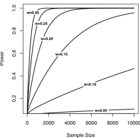
The statistical power of a hypothesis test is the probability of detecting a signifi-cant effect given that it exists in the data [24]. A test with low statistical power will often fail to detect a true effect resulting in a false negative error. This has long been recognized as a problem in constraint identification [87]. Statistical power depends on the sample sizeN, the degrees of freedom of the test, the significance threshold α (or type I error rate), and the expected effect sizew[24]. The effect size of a test defines a specific alternative hypothesis to compare against the null and indicates the mini-mum strength of correlation that is detectable by the hypothesis test. Running tests with small sample sizes or large degrees of freedom result in sampling distributions with high variance, leading to a corresponding decrease in statistical power.

The primary approach for preventing low-power statistical tests is to incorporate an upper limit on the degrees of freedom of the tests used in constraint identification. The first, and most widely used, approach of this type is the “rule of thumb”

Learning the Structure of Bayesian Networks with Constraint Satisfaction

University of Massachusetts Amherst

ScholarWorks@UMass Amherst

Learning the Structure of Bayesian Networks with

Constraint Satisfaction

Andrew Scott Fast

LEARNING THE STRUCTURE OF BAYESIAN

NETWORKS WITH CONSTRAINT SATISFACTION

LEARNING THE STRUCTURE OF BAYESIAN

NETWORKS WITH CONSTRAINT SATISFACTION

ACKNOWLEDGMENTS

ABSTRACT

LEARNING THE STRUCTURE OF BAYESIAN

NETWORKS WITH CONSTRAINT SATISFACTION

TABLE OF CONTENTS

LIST OF TABLES

LIST OF FIGURES

CHAPTER 1

INTRODUCTION

CHAPTER 2

BACKGROUND

2.1

Bayesian Networks

2.2

Overview of Structure Learning

2.3

Evaluating Structural Accuracy

CHAPTER 3

CONSTRAINT-BASED ALGORITHMS FOR LEARNING

BAYESIAN NETWORKS

3.1

Motivation

3.2

Constraint Identification

3.3

Alternative Skeleton Algorithms

3.4

Constraint-Based Edge Orientation

3.5

Hybrid Learning Algorithms

3.6

Refinement Algorithms

3.7

Summary

CHAPTER 4

ERRORS OF CONSTRAINT IDENTIFICATION

4.1

Introduction

4.2

Analysis of Errors

4.3

Focus on False Negative Errors

4.4

Sources of False Negative Errors