Random forests and artificial neural network for predicting daylight illuminance and energy consumption

Random Forests and Artificial Neural Network for Predicting Daylight

Illuminance and Energy Consumption

Muhammad Waseem Ahmad

_{, Jean-Laurent Hippolyte}

_{,Monjur Mourshed}

_{, Yacine Rezgui}

BRE Centre for Sustainable Engineering, School of Engineering,

Cardiff University, Cardiff, CF24 3AA, UK

_{[email protected];}

_{[email protected];}

3

_{[email protected];}

_{[email protected]}

Abstract

Predicting energy consumption and daylight illumi-nance plays an important part in building lighting

control strategies. The use of simplified or

data-driven methods is often preferred where a fast re-sponse is needed e.g. as a performance evaluation en-gine for advanced real-time control and optimization applications. In this paper we developed and then compared the performance of the widely-used Arti-ficial Neural Network (ANN) with Random Forest (RF), a recently developed ensemble-based algorithm. The target application was predicting the hourly en-ergy consumption and daylight illuminance values of a classroom in Cardiff, UK. Overall, RF performed better than ANN for predicting daylight illuminance;

with coefficients of determination (R2_{) of 0.9881 and}

0.9799 respectively. On the energy consumption test-ing dataset, ANN performed marginally better than

RF with R2_{values of 0.9973 and 0.9966 respectively.}

RF performs internal cross-validation and is relatively easy to tune as it has few tuning parameters. The paper also highlighted possible future research direc-tions.

Introduction

Buildings are responsible for 40% of the total global energy use and account for 30% of the total emission

of CO2, one of the greenhouse gases responsible for

anthropogenic climate change (Ahmad et al., 2016). To mitigate this, building regulations have been de-veloped or updated to reduce the impact of climate change and enhance the performance of buildings. With sustained reductions in a building’s heating and cooling demands, the energy used by artificial lighting increases in relative terms (Ahmad et al., 2015). Day-light is an essential part of our life, and building oc-cupants tend to prefer daylight over artificial lighting. It also provides a comfortable and effective learning environment in schools. An appropriate lighting level is necessary to satisfy both psychological and visual comfort conditions. Typically Venetian blinds have been used in buildings to control daylighting. In the literature, various automatic control strategies have been developed to enhance the thermal and

daylight-ing performance of occupied spaces. One example of this research work is Ahmad et al. (2015), the authors proposed a genetic algorithm based method to adjust the window blind position. On the other hand, energy prediction strategies are one of the core components of building energy control and operational strategies (Li and Wen, 2014).

In recent years, a number of prediction approaches, either detailed or simplified, have been proposed and applied for predicting building energy consumption and daylight illuminance. These approaches can be broadly classified into three categories i.e. numerical, analytical and predictive. Numerical approaches (e.g. EnergyPlus, DAYSIM, RADIANCE, TRNSYS, etc.) often enable the user to evaluate designs with reduced uncertainties. However, these methods do not per-form well in predicting the energy use and daylight-ing illuminance of occupied builddaylight-ings as it is difficult to model occupants’ behavior and how they interact with their buildings. On the other hand, predictive models (e.g. artificial neural networks, support

vec-tor machines, etc.) have been successfully applied

to predict the energy consumption of occupied build-ings. These models quickly perform predictions and thus are more suitable for real–time control purposes. In a recent review, Ahmad et al. (2016) discussed several computational intelligence (CI) techniques for HVAC systems. It was mentioned that significant ad-vances has been made in the past decades on the ap-plication of CI techniques for building energy appli-cations. Most of these techniques use historical data to train a model or develop expert rules. With the evolution towards Internet of Things (IoT), there is an abundance of data available from buildings, and therefore these CI techniques can easily be applied to enhance building energy performance. Random For-est (RF) has been less explored for building energy and daylight illuminance predictions. RF does not require much fine-tuning of their hyper-parameters, and default parameters often give better results than being fine-tuned. On the other hand, artificial neural networks (ANNs) have been extensively used for en-ergy and daylight predictions because of their fault–

study is to develop ANN and RF based models to predict the daylight illuminance and energy consump-tion of a classroom. This paper offers an alternative methodology to the existing energy consumption and illuminance prediction techniques.

Related work

In the literature, a large number of studies have fo-cussed on using machine learning techniques to pre-dict energy consumption. For building energy predic-tion, ANNs are the most popular choice among other computational intelligence techniques (Ahmad et al.,

2016). In two different studies, both Gonz´alez and

Zamarre˜no (2005) and Nizami and Al-Garni (1995)

used a simple neural network to predict hourly val-ues of building energy consumption by using weather and time stamp information as inputs to the mod-els. Nizami and Al-Garni (1995) compared the re-sults with a regression model and it was found that ANN performed better.

ANNs were also used by Kalogirou and Bojic (2000) to predict the energy use of a passive solar build-ing. The authors developed different modules to pre-dict outdoor and indoor air temperatures at next time step, as well as solar radiation and electrical heaters’ state. Kreider et al. (1995) reported on the use of recurrent neural networks to predict cooling and heating energy consumption. ANNs are also be-ing used to predict energy consumption for different climate zones by using envelope performance parame-ters, and heating and cooling degree days (Cheng-wen and Jian, 2010). Manufacturing industries show high fluctuations in their energy use and modeling energy consumption for these buildings could be a challeng-ing task. Azadeh et al. (2008) predicted the annual electricity consumption of this type of building by using an ANN, where the results demonstrated their suitability for this purpose.

To the best of our knowledge, there are only a few studies that focussed on the application of decision trees for energy prediction.Tso and Yau (2007) and Yu et al. (2010) studied the use of decision trees for predicting energy demand and residential building en-ergy performance respectively. Tso and Yau (2007) compared the results from neural network, decision trees, and regression analysis; and found that deci-sion trees could be viable alternatives to understand energy patterns. One key advantage of decision trees is that the user can generate accurate models with-out having any computational knowledge. Yu et al. (2010) found that decision trees can produce accu-rate models for predicting building energy use inten-sity levels. Ahmad et al. (2017) compared the results of neural network and random forest (an ensemble-based method) for predicting hourly energy consump-tion, and found that ANN performed marginally bet-ter than random forest.

ANNs are also being used for predicting daylight

il-luminance in buildings. Hu and Olbina (2011) pro-posed an illuminance-based Venetian blind control method and used ANNs to predict illuminance val-ues at two set-points. The author concluded that the proposed method has advantages for real-time blind control applications. Kazanasmaz et al. (2009) also used an ANN to determine daylight illuminance for

an office building. The authors used building and

weather parameters to predict illuminance values and found that the prediction accuracy of the model was approximately 98%. Ahmad et al. (2015) proposed a method for controlling Venetian blinds by using Ener-gyPlus as an evaluation engine. The authors stressed the need for a surrogate model to reduce the com-putational time required to run 1000s of simulations. Mourshed et al. (2011) studied the optimum design of artificial lighting and found that the search for an optimum design in a rugged solution space is a time consuming process, so there is a need to develop sur-rogate models.

Machine learning techniques

Random Forest

Random forests (RFs) are ensemble-based decision trees and were developed to overcome the shortcom-ings of traditional decision trees. In RF, like other ensemble learning techniques, the performance of a number of weak learners is boosted via a voting

scheme. The main hallmarks of random forest

in-clude; 1) bootstrap sampling – randomly selecting number of samples with replacement, 2) random fea-ture selection – randomly selecting only a small

num-ber of m features in the split of each node, 3) full

depth decision tree growing, and 4) Out-of-bag error estimation – calculating error on the samples which were not selected during bootstrap sampling (Jiang et al., 2009).

In RF, a M number of decision trees are generated

from a N number of training samples. For each

tree, bootstrap sampling is performed to create a new training set. The new training dataset is then used to create a fully grown decision tree without prun-ing by usprun-ing the ’classification and regression trees’ (CART) technique (Duda et al., 2012). Instead of using all available features at each split of the node,

only a small number of m features are randomly

se-lected. This procedure is then repeated untilM

deci-sion trees are created to form a randomly generated ”Forest”. For RF models, we used 1000 trees in the forest. One the hyper-parameters for RF is the

num-ber of randomly selected variablesmtryat each split

node; according to Breiman (2001), the recommended

value of mtry is equal to √pfor classification

prob-lems (where p being the total number of predictors).

The author also mentioned that mtry << p should

improve the performance of the model. For regression

Artificial Neural Network

Artificial Neural Networks (ANNs) learn the relation-ships between inputs and outputs by using a training dataset and do not need any information about the system as they are black-box models. The inspira-tion for ANNs comes from the funcinspira-tioning of bio-logical neurons. ANNs consist of a number of lay-ers of neuron-like processing units, which are inter-connected with each other. Different neural network strategies have been developed in the literature e.g. feed-forward, Hopfield, Elman, self-organising maps, and radial basis networks (Krenker et al., 2011). Feed-forward ANNs are the most widely used and generic neural network types and have been used for solving problems in various research fields.

This paper uses a feed-forward neural network trained by the Broyden-Flatcher-Goldfarb-Shano (BFGS) al-gorithm. In this study, only one hidden layer used, as more hidden layers did not improve the predic-tion power of the neural network. This concurs with Principe et al. (1999), who state that for most appli-cations, one hidden layer should be adequate. We also varied the number of neurons between 10-20 for both the energy consumption and daylight il-luminance models, by using the stepwise searching method. We found that for both models, using more than 10 neurons in the hidden layer did not signifi-cantly improve the accuracy of the models, so we used 10 hidden layer neurons. As the paper is focussed on random forest and its comparison with ANNs, the de-tails about searching the neurons in the hidden layer, number of hidden layers and training algorithms are not discussed here.

In order to develop machine learning models; we used the implementation of RF included in the scikit-learn module of the Python programming language, and the neurolab module for the development of artificial neural network.

Methodology

Energy model

A model of a classroom of a school building was cre-ated in EnergyPlus as a use case to develop and val-idate prediction models. The school building is lo-cated in Cardiff, UK and is a BREEAM excellent

(≈LEED platinum) rated building. The dimensions

of the classroom were 9.0 m (width)× 9.5 m (depth)

× 3.6 m (height). It was assumed that the

class-room has a 30% window-to-wall ratio on its

south-ern fa¸cade, which consists of a double glazing (3 mm

Generic PYR B Clear + 13 mm air gap + 3 mm Generic Clear). An interior Venetian blind was mod-eled on the window, which has a thermal conductivity of 0.9 W/mK and slat beam solar reflectance for both front and back sides were set to 0.8. The slat width was modeled as 2.5 cm and the slat angle was fixed

at 4◦. The illuminance levels were calculated at one

sensor point (SP), which was located in the middle of

the classroom at a height of 0.8 m.

Energy consumption and hourly illuminance values at the sensor point were obtained by running Energy-Plus simulations. The weather file for Cardiff, Wales, UK was used for these simulations. The cooling and heating demand of the model was met by using a pur-chased air system (ideal load air system). The system meets the energy demand by providing the required supply air capacity at the specified temperature. The heating and cooling set points are defined according

to CIBSE (2006) Guide A i.e. 22◦C and 24◦C for

heating and cooling respectively. 9 people were

mod-eled with an activity level of 60 W/m2_{. A}

continu-ous dimming control was modeled to control artificial lighting based on the lux level calculated at the SP. The sensor point has an illuminance set-point value of 300 lx (CIBSE, 2006). The outputs from the mod-els were energy consumption (sum of heating, cooling and lighting energy consumption) and daylight illu-minance at the SP. We also considered different in-put variables to improved the prediction accuracy of the machine learning models. The considered inputs variables were; solar altitude angle, solar azimuth an-gle, direct normal radiation, diffuse horizontal radia-tion, day of the week, hour of the day, month of the year, outdoor dry-bulb air temperature, wind speed, outdoor air relative humidity, window blind position, occupancy and previous hour values of daylight illu-minance and energy consumption.

Evaluation metrics

To evaluate the performance of the models, several metrics were calculated the testing data samples: the root mean squared error (RMSE), the coefficient of variation (CV), the mean absolute deviation and the

coefficient of determination (R2_{), as formalised in}

Equations (1) to (4). CV = qPN i=1(yi−yˆi)2 N ¯ y ×100 (1) RM SE= v u u u t N P i=1 (yi−ˆyi)2 N (2) M AD= 1 N N X i=1 |ˆyi−yi| (3) R2= 1− N P i=1 (yi−ˆyi)2 N P i=1 (yi−y)¯ 2 (4)

where ˆyi is the predicted output value, yi is the

ac-tual output variable for the ith_{sample in the testing}

subset, ¯y is the mean of the observed values and N

is the number of samples in the testing subset. The MAD metric calculates the average distance between

each data value and its mean for a given dataset. CV is a measure of variation in error with respect to the

actual consumption means,R2is used to evaluate the

closeness of fit, where perfectly fitted model will have

an R2 of 1. We have used RMSE as our primary

metric, and other performance metrics were used as tie breakers; they were considered only when RMSE did not provide any statistical difference between two prediction models.

Results and discussion

The variables used to train the prediction models, along with their maximum and minimum values, are

listed in Table 1. The variable importance plots

for energy consumption and daylight illuminance are shown in Figure 1. These plots were produced by re-placing each input variable in turn by random noise in the RF and then analyzing the deterioration of the performance of the random forest models. The result-ing deterioration is a measure of predictor’s impor-tance, for regression problems the most widely used score is the increase in the mean of the error of a tree (mean squared error) (Vincenzi et al., 2011). As shown in Figure 1, it is evident that for both en-ergy consumption and daylight illuminance, the pre-vious hour’s values are the most important variables. For energy consumption, other important variables include: occupancy schedule, outdoor dry-bulb tem-perature, indoor air temtem-perature, blind schedule, alti-tude angle, month of the year, diffuse solar radiation, hour of the day, azimuth angle, total transmitted so-lar radiation and direct soso-lar radiation. For daylight illuminance prediction; total transmitted solar radi-ation, direct solar radiradi-ation, altitude angle, diffuse solar radiation, azimuth angle, blind schedule, month of the year and hour of the day were the most influen-tial variables. We only used these input variables for further analysis (i.e tuning hyper-parameters, train-ing and testtrain-ing of models).

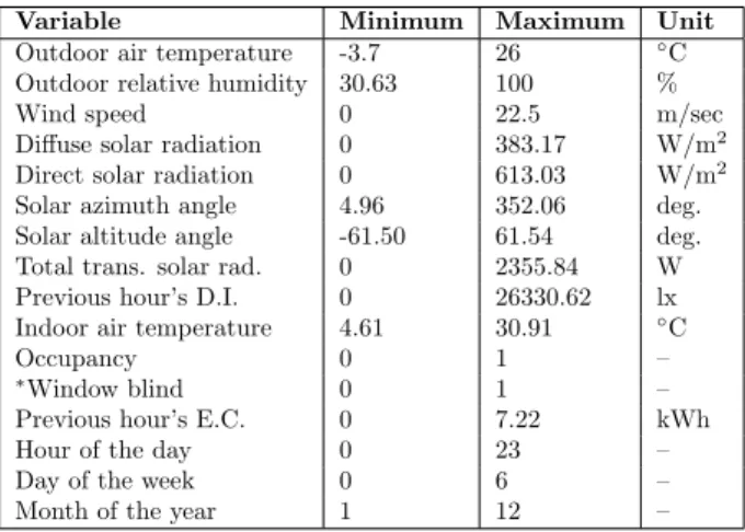
Table 1: Summary of the input variables considered in the model construction.

Variable Minimum Maximum Unit

Outdoor air temperature -3.7 26 ◦_C Outdoor relative humidity 30.63 100 %

Wind speed 0 22.5 m/sec

Diffuse solar radiation 0 383.17 W/m2 Direct solar radiation 0 613.03 W/m2 Solar azimuth angle 4.96 352.06 deg. Solar altitude angle -61.50 61.54 deg. Total trans. solar rad. 0 2355.84 W Previous hour’s D.I. 0 26330.62 lx Indoor air temperature 4.61 30.91 ◦_C

Occupancy 0 1 –

∗_{Window blind 0 1 –}

Previous hour’s E.C. 0 7.22 kWh

Hour of the day 0 23 –

Day of the week 0 6 –

Month of the year 1 12 –

Note: ∗_{Dichotomous variable}

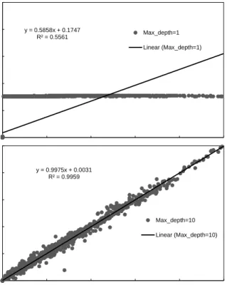
The observed effect of tree depth on the performance

0 0.1 0.2 0.3 0.4 0.5 P re . E ne rgy O c c u pa n c y Tem p In d o o r t e m p B lind S c he d ul e A lti Mo nth Diff Ho ur _Azi T ran s . S ol ar D ir e c t WS Da y RH 0 0.1 0.2 0.3 0.4 0.5 P re . Il lu T ran s . S ol ar Di re c t A lti Di ff A z i B lind S c he d ul e Mo nth Ho ur In do o r t em p T em p RH WS Da y O c c u pa n c y V aria bl e im po rtan c e for D.I. V aria bl e im po rtan c e for E .C.

Figure 1: Variable importance for energy consump-tion daylight illuminance predicconsump-tion models.

of a Random Forest models is shown in Figure 2 and

Table 2. For both cases, it was found that a

for-est constructed with deeper trees resulted in better accuracy. A maximum depth of 1 resulted in poor performance and led to under-fitting. From results, it is shown that using trees deeper than 10 levels did not enhance the performance significantly and there-fore, we used a maximum depth of 10 levels for both energy consumption and daylight illuminance predic-tion models. The forest with trees depth of 10 levels resulted in the lowest values of RMSE (0.0540), CV

(14.8952%), MAD (0.019) and a higher R2 (0.9959)

value for energy consumption. For daylight illumi-nance, using a tree depth of 10 levels resulted in

RMSE, CV and R2 values of 238.108, 36.429% and

0.9867 respectively.

Table 3 shows the effects of varying the number of features on the accuracy of the RF models.

the performance of RF models while varying the

num-ber of features. Increasingmtrycan improve the

pre-dictive performance of the RF model as there is a higher number of predictors being available each node of the tree. Contrary to the norm, we observed a de-terioration in the performance of the RF model when using more than 7 features. As shown in Table 3, the resulting CV values for the model with max fea-tures equal to 7 was 13.101% and 36.067% for energy

y = 0.5858x + 0.1747 R² = 0.5561 0 1 2 3 4 5 Max_depth=1 Linear (Max_depth=1) y = 0.9975x + 0.0031 R² = 0.9959 0 1 2 3 4 5 0 1 2 3 4 5 Max_depth=10 Linear (Max_depth=10) Expected E.C. (kWh) Pre d ic te d E.C. (k W h ) Pre d ic te d E.C. (k W h )

Figure 2: RF models for energy consumption with different maximum depths.

y = 0.458x + 343.26 R² = 0.7233 0 5000 10000 15000 20000 25000 Max_depth=1 Linear (Max_depth=1) y = 0.9592x + 21.948 R² = 0.9876 0 5000 10000 15000 20000 25000 0 5000 10000 15000 20000 25000 Max_depth=10 Linear (Max_depth=10) Pre d ic te d D.I (l u x) Pre d ic te d D.I (l u x)

Expected D.I. (lux)

Figure 3: RF models for daylight illuminance with different maximum depths.

Table 2: Maximum depth for RF

Max depth RMSE CV MAD R2

Energy consumption 1 0.5644 155.6710 0.238 0.5537 3 0.2166 59.7446 0.083 0.9342 5 0.1135 31.3014 0.043 0.9820 7 0.0741 20.4428 0.027 0.9923 10 0.0540 14.8952 0.019 0.9959 13 0.0496 13.6816 0.017 0.9966 15 0.0492 13.5786 0.016 0.9966 20 0.0491 13.5438 0.016 0.9966 Daylight Illuminance 1 1264.396 193.446 603.779 0.6260 3 650.598 99.538 194.066 0.9010 5 373.824 57.193 97.200 0.9673 7 271.102 41.477 60.927 0.9828 10 238.108 36.429 44.915 0.9867 13 235.500 36.030 41.058 0.9870 15 234.368 35.857 40.419 0.9871 20 234.936 35.944 40.368 0.9870

consumption and daylight illuminance respectively, which was higher than considering minimum feature

(mtry= 1, CVE.C = 37.818% and CVD.I= 61.205%)

and mtryE.C = 12 (CVE.C = 14.895%), mtryD.I =

9 (CVD.I = 36.429%). The results showed the same

behaviour for other performance metrics. Increasing

mtryalso reduced the diversity of the individual tree

in the forest and therefore the performance of the RF deteriorated when considering more than 7 features. It is also worth mentioning that the construction of an RF with more features is computationally inten-sive and hence slower.

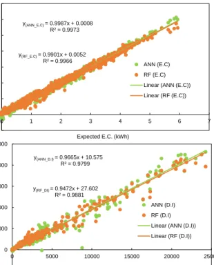
To evaluate the accuracy and generalization capabil-ities of the developed models, both models were used to predict energy consumption and daylight

illumi-nance on an unseen dataset (i.e. the dataset was

not used during the training or validation stages). The results from both models are shown in Figure 4.

Moreover, RMSE and R2_{of the testing and validation}

samples using RF and ANN models were compared, and are shown in Table 4. From Table 4 and Figure 4,

Table 3: Maximum Features for RF

Max features RMSE CV MAD R2

Energy consumption 1 0.137 37.818 0.060 0.9736 3 0.064 17.833 0.024 0.9942 5 0.051 14.199 0.019 0.9963 7 0.048 13.101 0.017 0.9968 10 0.049 13.544 0.017 0.9966 12 0.054 14.895 0.019 0.9959 Daylight Illuminance 1 400.046 61.205 86.806 0.9626 3 270.917 41.449 52.871 0.9828 5 242.970 37.173 47.027 0.9862 7 235.738 36.067 45.335 0.9870 8 236.302 36.153 44.645 0.9870 9 238.108 36.429 44.915 0.9867

Table 4: Comparison of ANN and RF for validation and testing datasets

Validation Testing

Model RMSE R2 _{RMSE R}2

RF (E.C) 0.048 0.9968 0.0559 0.9966

ANN (E.C) 0.043 0.9975 0.0493 0.9973

RF (D.I) 235.738 0.9870 227.87 0.9881

ANN (D.I) 282.354 0.9814 278.498 0.9799

it is evident that the Random Forest model performed better at predicting daylight illuminance, had lower

RMSE values and higher R2 _{values. On the other}

hand, ANN performed slightly better while predict-ing energy consumption. Predictpredict-ing daylight illumi-nance was a challenging task as the illumiillumi-nance at SP has drastic fluctuations. RF models performed well at predicting both higher and lower values, whereas ANN struggled to predict particularly lower values. There were even two high values of daylight illumi-nance which the ANN model predicted as values close to zero. One of the advantages of RF, as an ensemble algorithm, is that it can efficiently deal with any miss-ing values in the input values. Both studied models did capture the relationship between input and out-put variables and can be used as evaluation engines.

y(ANN_E.C) = 0.9987x + 0.0008 R² = 0.9973 y(RF_E.C) = 0.9901x + 0.0052 R² = 0.9966 -1 0 1 2 3 4 5 6 7 0 1 2 3 4 5 6 7 ANN (E.C) RF (E.C) Linear (ANN (E.C)) Linear (RF (E.C)) y(ANN_D.I) = 0.9665x + 10.575 R² = 0.9799 y(RF_DI) = 0.9472x + 27.602 R² = 0.9881 -5000 0 5000 10000 15000 20000 25000 0 5000 10000 15000 20000 25000 ANN (D.I) RF (D.I) Linear (ANN (D.I)) Linear (RF (D.I)) Pre d ic te d D.I (l u x ) Expected E.C. (kWh)

Expected D.I. (lux)

Pre d ic te d E.C. (k W h )

Figure 4: Testing results for RF and ANN models

The results showed that both models can be valu-able computational intelligence tools to predict en-ergy consumption and daylight illuminance. We also found that the training time of the RF model was much less than the ANN model (a few seconds versus a few minutes). This time may vary from problem

to problem and also depends on other factors (e.g. number of trees in the forest, tree depth, number of random features selected at each split). Our results concur with Siroky et al. (2009), who state that Ran-dom Forests are faster to train and tune than other ML techniques.

Conclusions

The paper presented two machine learning algorithms to predict energy consumption and daylight illumi-nance, based on a simulation model of a classroom. Based on the evaluation metrics of RMSE, CV, MAD

and R2_{, it was found that the developed models can}

be feasible and effective for predicting the hourly daylight illuminance at a set-point and energy con-sumption. On the testing dataset, ANN performed marginally better than RF for predicting energy con-sumption with a RMSE value of 0.0559 as compared to 0.0493. Whereas, on daylight illuminance predic-tion’s validation dataset, RF model provided better results than the ANN model. The paper also used RF as a method to calculate variable importance score, which is a useful method for dimensionality reduc-tion in order to improve model’s performance on high-dimensional datasets.

Whilst the paper was focussed on developing ML models for a specific classroom, the study will be extended in the future to include a diverse range of building types. In future, the performance of the pro-posed models will be compared with other ensemble based algorithms e.g. Gradient Boosted Regression Trees (Friedman, 2002) and Extremely Randomised Trees (Geurts et al., 2006). In the paper, the models were developed by using a Test Reference year (TRY weather file), however, in future actual weather con-ditions will be used to replicate the proposed work.

Acknowledgement

The authors acknowledge financial support from the European Commission Seventh Framework Pro-gramme (FP7), grant reference – 609154.

References

Ahmad, M., M. Mourshed, J.-L. Hippolyte,

Y. Rezgui, and H. Li (2015). Optimising the

scheduled operation of window blinds to enhance

occupant comfort. In Proceedings of BS2015:

14th Conference of International Building

Perfor-mance Simulation Association, Hyderabad, India,

pp. 2393–2400.

Ahmad, M. W., M. Mourshed, D. Mundow,

M. Sisinni, and Y. Rezgui (2016). Building energy metering and environmental monitoring – a state-of-the-art review and directions for future research.

Energy and Buildings 120, 85 – 102.

Ahmad, M. W., M. Mourshed, and Y. Rezgui (2017). Trees vs neurons: Comparison between random

forest and ANN for high-resolution prediction of

building energy consumption. Energy and

Build-ings 147, 77 – 89.

Ahmad, M. W., M. Mourshed, B. Yuce, and

Y. Rezgui (2016). Computational intelligence

tech-niques for hvac systems: A review. Building

Simu-lation 9(4), 359–398.

Azadeh, A., S. Ghaderi, and S. Sohrabkhani (2008). Annual electricity consumption forecasting by neu-ral network in high energy consuming

indus-trial sectors. Energy Conversion and

Manage-ment 49(8), 2272 – 2278.

Breiman, L. (2001). Random forests. Machine

learn-ing 45(1), 5–32.

Cheng-wen, Y. and Y. Jian (2010, May). Applica-tion of ann for the predicApplica-tion of building energy consumption at different climate zones with hdd

and cdd. InFuture Computer and Communication

(ICFCC), 2010 2nd International Conference on,

Volume 3, pp. 286–289.

CIBSE, G. A. (2006). Environmental design. The

Chartered Institution of Building Services

Engi-neers, London.

Duda, R. O., P. E. Hart, and D. G. Stork (2012).

Pattern classification. John Wiley & Sons.

Friedman, J. H. (2002). Stochastic gradient boosting.

Computational Statistics & Data Analysis 38(4),

367–378.

Geurts, P., D. Ernst, and L. Wehenkel (2006).

Ex-tremely randomized trees.Machine learning 63(1),

3–42.

Gonz´alez, P. A. and J. M. Zamarre˜no (2005).

Pre-diction of hourly energy consumption in buildings

based on a feedback artificial neural network.

En-ergy and Buildings 37(6), 595 – 601.

Hu, J. and S. Olbina (2011). Illuminance-based slat angle selection model for automated control of split

blinds.Building and Environment 46(3), 786 – 796.

Jiang, R., W. Tang, X. Wu, and W. Fu (2009). A ran-dom forest approach to the detection of epistatic

interactions in case-control studies. BMC

bioinfor-matics 10(1), 1.

Kalogirou, S. A. and M. Bojic (2000). Artificial neural networks for the prediction of the energy

consump-tion of a passive solar building. Energy 25(5), 479

– 491.

Kazanasmaz, T., M. Gnaydin, and S. Binol (2009). Artificial neural networks to predict daylight

illu-minance in office buildings. Building and

Environ-ment 44(8), 1751 – 1757.

Kreider, J., D. Claridge, P. Curtiss, R. Dodier, J. Haberl, and M. Krarti (1995). Building energy use prediction and system identification using

re-current neural networks. Journal of solar energy

engineering 117(3), 161–166.

Krenker, A., J. Bester, and A. Kos (2011).

Intro-duction to the artificial neural networks.

Artifi-cial neural networks: methodological advances and

biomedical applications, 1–18.

Li, X. and J. Wen (2014). Review of building energy

modeling for control and operation.Renewable and

Sustainable Energy Reviews 37, 517–537.

Mourshed, M., S. Shikder, and A. D. Price (2011). Phi-array: A novel method for fitness visualiza-tion and decision making in evoluvisualiza-tionary design

optimization. Advanced Engineering

Informat-ics 25(4), 676 – 687. Special Section: Advances

and Challenges in Computing in Civil and Build-ing EngineerBuild-ing.

Nizami, S. J. and A. Z. Al-Garni (1995). Forecasting electric energy consumption using neural networks.

Energy Policy 23(12), 1097 – 1104.

Principe, J. C., N. R. Euliano, and W. C. Lefebvre

(1999).Neural and adaptive systems: fundamentals

through simulations with CD-ROM. John Wiley &

Sons, Inc.

Siroky, D. S. et al. (2009). Navigating random

forests and related advances in algorithmic mod-eling. Statistics Surveys 3, 147–163.

Tso, G. K. and K. K. Yau (2007). Predicting electric-ity energy consumption: A comparison of regres-sion analysis, deciregres-sion tree and neural networks.

Energy 32(9), 1761 – 1768.

Vincenzi, S., M. Zucchetta, P. Franzoi, M. Pellizzato, F. Pranovi, G. A. D. Leo, and P. Torricelli (2011). Application of a random forest algorithm to pre-dict spatial distribution of the potential yield of ruditapes philippinarum in the venice lagoon, italy.

Ecological Modelling 222(8), 1471 – 1478.

Yu, Z., F. Haghighat, B. C. Fung, and H. Yoshino (2010). A decision tree method for building energy

demand modeling. Energy and Buildings 42(10),