Automatic time series forecasting: the forecast package for R.

(1)

ISSN 1440-771X

Department of Econometrics and Business Statistics

http://www.buseco.monash.edu.au/depts/ebs/pubs/wpapers/

Automatic time series forecasting:

the forecast package for R

Rob J Hyndman and Yeasmin Khandakar

June 2007

(2)

Automatic time series forecasting:

the forecast package for R

Rob J Hyndman

Department of Econometrics and Business Statistics, Monash University, VIC 3800

Australia.

Email: [email protected]

Yeasmin Khandakar

Department of Econometrics and Business Statistics, Monash University, VIC 3800

Australia.

Email: [email protected]

11 June 2007

(3)

Automatic time series forecasting:

the forecast package for R

Abstract: Automatic forecasts of large numbers of univariate time series are often needed in business and other contexts. We describe two automatic forecasting algorithms that have been implemented in theforecast package for R. The first is based on innovations state space models that underly exponential smoothing methods. The second is a step-wise algorithm for forecasting with ARIMA models. The algorithms are applicable to both seasonal and non-seasonal data, and are compared and illustrated using four real time series. We also briefly describe some of the other functionality available in theforecast package.

Keywords: ARIMA models, automatic forecasting, exponential smoothing, prediction inter-vals, state space models, time series, R.

(4)

Automatic time series forecasting: the forecast package for R

Automatic forecasts of large numbers of univariate time series are often needed in busi-ness. It is common to have over one thousand product lines that need forecasting at least monthly. Even when a smaller number of forecasts is required, there may be nobody suitably trained in the use of time series models to produce them. In these circumstances, an automatic forecasting algorithm is an essential tool. Automatic forecasting algorithms must determine an appropriate time series model, estimate the parameters and compute the forecasts. They must be robust to unusual time series patterns, and applicable to large numbers of series without user intervention. The most popular automatic forecasting al-gorithms are based on either exponential smoothing or ARIMA models.

In this article, we discuss the implementation of two automatic univariate forecasting methods in the forecast package forR. Theforecast package is part of theforecasting

bundle which also contains the packagesfma andMcomp. Theforecast package con-tains functions for univariate forecasting, while the other two packages contain large col-lections of real time series data that are suitable for testing forecasting methods. Thefma

package contains the 90 data sets from Makridakis et al. (1998), and theMcomppackage contains the 1001 time series from the M-competition (Makridakis et al., 1982) and the 3003 time series from the M3-competition (Makridakis and Hibon, 2000).

The forecast package implements automatic forecasting using exponential smoothing, ARIMA models, the Theta method (Assimakopoulos and Nikolopoulos, 2000), cubic splines (Hyndman et al., 2005a), as well as other common forecasting methods. In this ar-ticle, we only discuss the exponential smoothing approach (in Section 1) and the ARIMA modelling approach (in Section 2) to automatic forecasting.

1 Exponential smoothing

Although exponential smoothing methods have been around since the 1950s, a mod-elling framework incorporating procedures for model selection was not developed until relatively recently. Ord et al. (1997), Hyndman et al. (2002) and Hyndman et al. (2005b) have shown that all exponential smoothing methods (including non-linear methods) are optimal forecasts from innovations state space models.

Exponential smoothing methods were originally classified by Pegels’ (1969) taxonomy.

(5)

This was later extended by Gardner (1985), modified by Hyndman et al. (2002), and ex-tended again by Taylor (2003), giving a total of fifteen methods seen in the following table.

Seasonal Component

Trend N A M

Component (None) (Additive) (Multiplicative)

N (None) N,N N,A N,M

A (Additive) A,N A,A A,M

A_d (Additive damped) A_d,N A_d,A A_d,M

M (Multiplicative) M,N M,A M,M

M_d (Multiplicative damped) M_d,N M_d,A M_d,M

Some of these methods are better known under other names. For example, cell (N,N) describes the simple exponential smoothing (or SES) method, cell (A,N) describes Holt’s linear method, and cell (A_d,N) describes the damped trend method. The additive Holt-Winters’ method is given by cell (A,A) and the multiplicative Holt-Holt-Winters’ method is given by cell (A,M). The other cells correspond to less commonly used but analogous methods.

1.1 Point forecasts for all methods

We denote the observed time series byy1, y2, . . . , yn. A forecast ofyt+hbased on all of the

data up to timetis denoted byyˆt+h|t. To illustrate the method, we give the point forecasts

and updating equations for method (A,A), the Holt-Winters’ additive method:

Level: ℓt = α(yt−st−m) + (1−α)(ℓt−1+bt−1) (1a)

Growth: bt = β∗(ℓt−ℓt−1) + (1−β∗)bt−1 (1b)

Seasonal: st = γ(yt−ℓt−1−bt−1) + (1−γ)st−m (1c)

Forecast: yˆ_t+h|t = ℓt+bth+s_t₋_m+h+m. (1d)

(6)

wherem is the length of seasonality (e.g., the number of months or quarters in a year),

ℓtrepresents the level of the series,btdenotes the growth,stis the seasonal component, ˆ

yt+h|tis the forecast forhperiods ahead, andh+m =

(h−1)modm

+ 1. To use method (1), we need values for the initial statesℓ0, b0 ands1−m, . . . , s0, and for the smoothing

parametersα,β∗andγ. All of these will be estimated from the observed data.

Equation (1c) is slightly different from the usual Holt-Winters equations such as those in Makridakis et al. (1998) or Bowerman et al. (2005). These authors replace (1c) with

st=γ∗(yt−ℓt) + (1−γ∗)st−m.

Ifℓtis substituted using (1a), we obtain

st=γ∗(1−α)(yt−ℓt−1−bt−1) +{1−γ∗(1−α)}st−m.

Thus, we obtain identical forecasts using this approach by replacingγin (1c) withγ∗(1−

α). The modification given in (1c) was proposed by Ord et al. (1997) to make the state space formulation simpler. It is equivalent to Archibald’s (1990) variation of the Holt-Winters’ method.

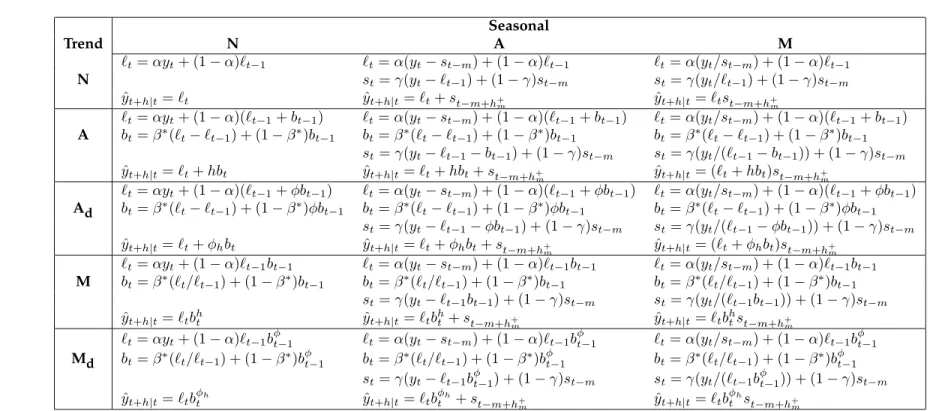
Table 1 gives recursive formulae for computing point forecastshperiods ahead for all of the exponential smoothing methods. In each case, ℓt denotes the series level at time t, bt denotes the slope at time t, st denotes the seasonal component of the series at time t and m denotes the number of seasons in a year; α, β∗, γ and φ are constants, and

φh =φ+φ2+· · ·+φh.

Some interesting special cases can be obtained by setting the smoothing parameters to extreme values. For example, ifα= 0, the level is constant over time; ifβ∗ = 0, the slope is constant over time; and ifγ = 0, the seasonal pattern is constant over time. At the other extreme, na¨ıve forecasts (i.e., yˆt+h|t = ytfor allh) are obtained using the (N,N) method

with α = 1. Finally, the additive and multiplicative trend methods are special cases of their damped counterparts obtained by lettingφ= 1.

(7)

A u to m a tic tim e se rie s fo re ca st in g : th e fo re ca st p a ck a g e fo r R Seasonal Trend N A M ℓt=αyt+ (1−α)ℓt−1 ℓt=α(yt−st−m) + (1−α)ℓt−1 ℓt=α(yt/st−m) + (1−α)ℓt−1 N st=γ(yt−ℓt−1) + (1−γ)st−m st=γ(yt/ℓt−1) + (1−γ)st−m ˆ yt+h|t=ℓt yˆt+h|t=ℓt+s_t₋_m+h+m yˆt+h|t=ℓtst−m+h+m ℓt=αyt+ (1−α)(ℓt−1+bt−1) ℓt=α(yt−st−m) + (1−α)(ℓt−1+bt−1) ℓt=α(yt/st−m) + (1−α)(ℓt−1+bt−1) A bt=β∗(ℓt−ℓt−1) + (1−β∗)bt−1 bt=β∗(ℓt−ℓt−1) + (1−β∗)bt−1 bt=β∗(ℓt−ℓt−1) + (1−β∗)bt−1 st=γ(yt−ℓt−1−bt−1) + (1−γ)st−m st=γ(yt/(ℓt−1−bt−1)) + (1−γ)st−m ˆ yt+h|t=ℓt+hbt yˆt+h|t=ℓt+hbt+s_t₋_m+h+m yˆt+h|t= (ℓt+hbt)st−m+h+m ℓt=αyt+ (1−α)(ℓt−1+φbt−1) ℓt=α(yt−st−m) + (1−α)(ℓt−1+φbt−1) ℓt=α(yt/st−m) + (1−α)(ℓt−1+φbt−1) A_d bt=β∗(ℓt−ℓt−1) + (1−β∗)φbt−1 bt=β∗(ℓt−ℓt−1) + (1−β∗)φbt−1 bt=β∗(ℓt−ℓt−1) + (1−β∗)φbt−1 st=γ(yt−ℓt−1−φbt−1) + (1−γ)st−m st=γ(yt/(ℓt−1−φbt−1)) + (1−γ)st−m ˆ yt+h|t=ℓt+φhbt yˆt+h|t=ℓt+φhbt+st−m+h+m yˆt+h|t= (ℓt+φhbt)st−m+h + m ℓt=αyt+ (1−α)ℓt−1bt−1 ℓt=α(yt−st−m) + (1−α)ℓt−1bt−1 ℓt=α(yt/st−m) + (1−α)ℓt−1bt−1 M bt=β∗(ℓt/ℓt−1) + (1−β∗)bt−1 bt=β∗(ℓt/ℓt−1) + (1−β∗)bt−1 bt=β∗(ℓt/ℓt−1) + (1−β∗)bt−1 st=γ(yt−ℓt−1bt−1) + (1−γ)st−m st=γ(yt/(ℓt−1bt−1)) + (1−γ)st−m ˆ yt+h|t=ℓtbth yˆt+h|t=ℓtbht +st−m+h+m yˆt+h|t=ℓtb h tst−m+h+m ℓt=αyt+ (1−α)ℓt−1b φ t−1 ℓt=α(yt−st−m) + (1−α)ℓt−1b φ t−1 ℓt=α(yt/st−m) + (1−α)ℓt−1b φ t−1 M_d bt=β∗(ℓt/ℓt−1) + (1−β∗)bφt−1 bt=β∗(ℓt/ℓt−1) + (1−β∗)bφt−1 bt=β∗(ℓt/ℓt−1) + (1−β∗)bφt−1 st=γ(yt−ℓt−1bφ_t₋1) + (1−γ)st−m st=γ(yt/(ℓt−1bφ_t₋1)) + (1−γ)st−m ˆ yt+h|t=ℓtb φh t yˆt+h|t=ℓtb φh t +st−m+h+ m yˆt+h|t=ℓtb φh t st−m+h+ m

Table 1: Formulae for recursive calculations and point forecasts. In each case, ℓt denotes the series level at time t, bt denotes the slope at time t, st denotes the seasonal component of the series at time t, andm denotes the number of seasons in a year; α, β∗, γ andφare constants, φh =φ+φ2 +· · ·+φh_and_h+ m = (h−1)modm + 1. H y n d m a n a n d K h a n d a ka r: J u n e 2 0 0 7

5

(8)

1.2 Innovations state space models

For each exponential smoothing method in Table 1, Hyndman et al. (2002) describe two possible innovations state space models, one corresponding to a model with additive errors and the other to a model with multiplicative errors. If the same parameter values are used, these two models give equivalent point forecasts, although different prediction intervals. Thus there are 30 potential models described in this classification.

Historically, the nature of the error component has often been ignored, because the dis-tinction between additive and multiplicative errors makes no difference to point fore-casts.

We are careful to distinguish exponential smoothingmethods from the underlying state space models. An exponential smoothing method is an algorithm for producing point forecasts only. The underlying stochastic state space model gives the same point fore-casts, but also provides a framework for computing prediction intervals and other prop-erties.

To distinguish the models with additive and multiplicative errors, we add an extra letter to the front of the method notation. The triplet (E,T,S) refers to the three components: error, trend and seasonality. So the model ETS(A,A,N) has additive errors, additive trend and no seasonality—in other words, this is Holt’s linear method with additive errors. Similarly, ETS(M,M_d,M) refers to a model with multiplicative errors, a damped multi-plicative trend and multimulti-plicative seasonality. The notation ETS(·,·,·) helps in remember-ing the order in which the components are specified.

Once a model is specified, we can study the probability distribution of future values of the series and find, for example, the conditional mean of a future observation given knowledge of the past. We denote this as µ_t+h|t = E(yt+h | xt), wherext contains the

unobserved components such as ℓt, btandst. Forh = 1 we useµt ≡ µt+1|t as a

short-hand notation. For many models, these conditional means will be identical to the point forecasts given in Table 1, so thatµt+h|t = ˆyt+h|t. However, for other models (those with

multiplicative trend or multiplicative seasonality), the conditional mean and the point forecast will differ slightly forh ≥2.

We illustrate these ideas using the damped trend method of Gardner and McKenzie

(9)

(1985).

Additive error model: ETS(A,Ad,N)

Letµt = ˆyt = ℓt−1+bt−1 denote the one-step forecast ofytassuming that we know the

values of all parameters. Also, letεt =yt−µtdenote the one-step forecast error at time t. From the equations in Table 1, we find that

yt = ℓt−1+φbt−1+εt (2)

ℓt = ℓt−1+φbt−1+αεt (3)

bt = φbt−1+β∗(ℓt−ℓt−1−φbt−1) =φbt−1+αβ∗εt. (4)

We simplify the last expression by settingβ=αβ∗. The three equations above constitute a state space model underlying the damped Holt’s method. Note that it is aninnovations

state space model (Anderson and Moore, 1979; Aoki, 1987) because the same error term appears in each equation. We can write it in standard state space notation by defining the state vector asx_t_{= (ℓ}_t_{, b}_t₎′_{and expressing (2)–(4) as}

yt = [1 φ]xt−1+εt (5a) x_t ₌   1 φ 0 φ  xt−1+   α β  εt. (5b)

The model is fully specified once we state the distribution of the error termεt. Usually

we assume that these are independent and identically distributed, following a normal distribution with mean 0 and varianceσ2

, which we write asεt∼NID(0, σ2).

Multiplicative error model: ETS(M,Ad,N)

A model with multiplicative error can be derived similarly, by first settingεt = (yt− µt)/µt, so that εt is the relative error. Then, following a similar approach to that for

additive errors, we find

yt = (ℓt−1+φbt−1)(1 +εt)

(10)

Automatic time series forecasting: the forecast package for R ℓt = (ℓt−1+φbt−1)(1 +αεt) bt = φbt−1+β(ℓt−1+φbt−1)εt, or yt = [1 φ]xt−1(1 +εt) x_t ₌   1 φ 0 φ  xt−1+ [1 φ]xt−1   α β  εt.

Again we assume thatεt ∼NID(0, σ2).

Of course, this is a nonlinear state space model, which is usually considered difficult to handle in estimating and forecasting. However, that is one of the many advantages of the innovations form of state space models — we can still compute forecasts, the likelihood and prediction intervals for this nonlinear model with no more effort than is required for the additive error model.

1.3 State space models for all exponential smoothing methods

We now give the state space models for all 30 exponential smoothing variations. The general model involves a state vector x_t _{= (ℓ}_t_{, b}_t_, _s_t_{, s}_t₋₁_{, . . . , s}_t₋_m₊₁₎′ _{and state space}

equations of the form

yt = w(xt−1) +r(xt−1)εt (6a)

x_t ₌ _f₍x_t₋₁_{) +}_g(x_t₋₁_)ε_t _(6b)

where{εt}is a Gaussian white noise process with mean zero and varianceσ2, andµt= w(x_t₋1). The model with additive errors hasr(xt−1) = 1, so thatyt=µt+εt. The model

with multiplicative errors hasr(x_t₋₁_{) =}_µ_t_{, so that}_y_t₌_µ_t_{(1 +}_ε_t₎_{. Thus,}_ε_t_{= (y}_t₋_µ_t_)/µ_t

is the relative error for the multiplicative model. The models are not unique. Clearly, any value ofr(x_t₋₁₎_{will lead to identical point forecasts for}_y_t_.

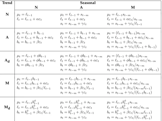
All of the methods in Table 1 can be written in the form (6a) and (6b). The underlying equations for additive error models are given in Table 2. We use β = αβ∗ to simplify the notation. Multiplicative error models are obtained by replacing εt with µtεtin the

(11)

A u to m a tic tim e se rie s fo re ca st in g : th e fo re ca st p a ck a g e fo r R Trend Seasonal N A M N µt=ℓt−1 µt=ℓt−1+st−m µt=ℓt−1st−m ℓt=ℓt−1+αεt ℓt=ℓt−1+αεt ℓt=ℓt−1+αεt/st−m st=st−m+γεt st=st−m+γεt/ℓt−1 µt=ℓt−1+bt−1 µt=ℓt−1+bt−1+st−m µt= (ℓt−1+bt−1)st−m A ℓt=ℓt−1+bt−1+αεt ℓt=ℓt−1+bt−1+αεt ℓt=ℓt−1+bt−1+αεt/st−m bt=bt−1+βεt bt=bt−1+βεt bt=bt−1+βεt/st−m st=st−m+γεt st=st−m+γεt/(ℓt−1+bt−1) µt=ℓt−1+φbt−1 µt=ℓt−1+φbt−1+st−m µt= (ℓt−1+φbt−1)st−m A_d ℓt=ℓt−1+φbt−1+αεt ℓt=ℓt−1+φbt−1+αεt ℓt=ℓt−1+φbt−1+αεt/st−m bt=φbt−1+βεt bt=φbt−1+βεt bt=φbt−1+βεt/st−m st=st−m+γεt st=st−m+γεt/(ℓt−1+φbt−1) µt=ℓt−1bt−1 µt=ℓt−1bt−1+st−m µt=ℓt−1bt−1st−m M ℓt=ℓt−1bt−1+αεt ℓt=ℓt−1bt−1+αεt ℓt=ℓt−1bt−1+αεt/st−m bt=bt−1+βεt/ℓt−1 bt=bt−1+βεt/ℓt−1 bt=bt−1+βεt/(st−mℓt−1) st=st−m+γεt st=st−m+γεt/(ℓt−1bt−1) µt=ℓt−1b φ t−1 µt=ℓt−1b φ t−1+st−m µt=ℓt−1b φ t−1st−m M_d ℓt=ℓt−1b φ t−1+αεt ℓt=ℓt−1b φ t−1+αεt ℓt=ℓt−1b φ t−1+αεt/st−m bt=bφt−1+βεt/ℓt−1 bt=bφt−1+βεt/ℓt−1 bt=bφt−1+βεt/(st−mℓt−1) st=st−m+γεt st=st−m+γεt/(ℓt−1bφ_t₋1)

Table 2:State space equations for each additive error model in the classification.

H y n d m a n a n d K h a n d a ka r: J u n e 2 0 0 7

9

(12)

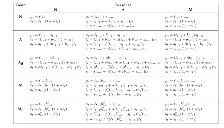
A u to m a tic tim e se rie s fo re ca st in g : th e fo re ca st p a ck a g e fo r R Trend Seasonal N A M N µt=ℓt−1 µt=ℓt−1+st−m µt=ℓt−1st−m ℓt=ℓt−1(1 +αεt) ℓt=ℓt−1+α(ℓt−1+st−m)εt ℓt=ℓt−1(1 +αεt) st=st−m+γ(ℓt−1+st−m)εt st=st−m(1 +γεt) µt=ℓt−1+bt−1 µt=ℓt−1+bt−1+st−m µt= (ℓt−1+bt−1)st−m A ℓt= (ℓt−1+bt−1)(1 +αεt) ℓt=ℓt−1+bt−1+α(ℓt−1+bt−1+st−m)εt ℓt= (ℓt−1+bt−1)(1 +αεt) bt=bt−1+β(ℓt−1+bt−1)εt bt=bt−1+β(ℓt−1+bt−1+st−m)εt bt=bt−1+β(ℓt−1+bt−1)εt st=st−m+γ(ℓt−1+bt−1+st−m)εt st=st−m(1 +γεt) µt=ℓt−1+φbt−1 µt=ℓt−1+φbt−1+st−m µt= (ℓt−1+φbt−1)st−m A_d ℓt= (ℓt−1+φbt−1)(1 +αεt) ℓt=ℓt−1+φbt−1+α(ℓt−1+φbt−1+st−m)εt ℓt= (ℓt−1+φbt−1)(1 +αεt) bt=φbt−1+β(ℓt−1+φbt−1)εt bt=φbt−1+β(ℓt−1+φbt−1+st−m)εt bt=φbt−1+β(ℓt−1+φbt−1)εt st=st−m+γ(ℓt−1+φbt−1+st−m)εt st=st−m(1 +γεt) µt=ℓt−1bt−1 µt=ℓt−1bt−1+st−m µt=ℓt−1bt−1st−m M ℓt=ℓt−1bt−1(1 +αεt) ℓt=ℓt−1bt−1+α(ℓt−1bt−1+st−m)εt ℓt=ℓt−1bt−1(1 +αεt) bt=bt−1(1 +βεt) bt=bt−1+β(ℓt−1bt−1+st−m)εt/ℓt−1 bt=bt−1(1 +βεt) st=st−m+γ(ℓt−1bt−1+st−m)εt st=st−m(1 +γεt) µt=ℓt−1b φ t−1 µt=ℓt−1b φ t−1+st−m µt=ℓt−1b φ t−1st−m M_d ℓt=ℓt−1b φ t−1(1 +αεt) ℓt=ℓt−1b φ t−1+α(ℓt−1b φ t−1+st−m)εt ℓt=ℓt−1b φ t−1(1 +αεt) bt=bφt−1(1 +βεt) bt=bφt−1+β(ℓt−1bφ_t₋1+st−m)εt/ℓt−1 bt=bφt−1(1 +βεt) st=st−m+γ(ℓt−1bφ_t₋1+st−m)εt st=st−m(1 +γεt)

Table 3: State space equations for each multiplicative error model in the classification.

H y n d m a n a n d K h a n d a ka r: J u n e 2 0 0 7

1

0

(13)

equations of Table 2. The resulting multiplicative error equations are given in Table 3. Some of the combinations of trend, seasonality and error can occasionally lead to numer-ical difficulties; specifnumer-ically, any model equation that requires division by a state compo-nent could involve division by zero. This is a problem for models with additive errors and either multiplicative trend or multiplicative seasonality, as well as for the model with multiplicative errors, multiplicative trend and additive seasonality. These models should therefore be used with caution.

The multiplicative error models are useful when the data are strictly positive, but are not numerically stable when the data contain zeros or negative values. So when the time series is not strictly positive, only the six fully additive models may be applied.

The point forecasts given in Table 1 are easily obtained from these models by iter-ating equations (6a) and (6b) for t = n + 1, n + 2, . . . , n + h, setting εn+j = 0 for j = 1, . . . , h. In most cases (notable exceptions being models with multiplicative sea-sonality or multiplicative trend forh≥2), the point forecasts can be shown to be equal to

µ_t+h|t=E(yt+h |xt), the conditional expectation of the corresponding state space model.

The models also provide a means of obtaining prediction intervals. In the case of the linear models, where the forecast distributions are normal, we can derive the conditional variance vt+h|t = Var(yt+h | xt) and obtain prediction intervals accordingly. This

ap-proach also works for many of the nonlinear models. Detailed derivations of the results for many models are given in Hyndman et al. (2005b).

A more direct approach that works for all of the models is to simply simulate many fu-ture sample paths conditional on the last estimate of the state vector,x_t_{. Then prediction}

intervals can be obtained from the percentiles of the simulated sample paths. Point fore-casts can also be obtained in this way by taking the average of the simulated values at each future time period. An advantage of this approach is that we generate an estimate of the complete predictive distribution, which is especially useful in applications such as inventory planning, where expected costs depend on the whole distribution.

(14)

1.4 Estimation

In order to use these models for forecasting, we need to know the values ofx₀ _{and the}

parametersα, β, γ and φ. It is easy to compute the likelihood of the innovations state space model (6), and so obtain maximum likelihood estimates. Ord et al. (1997) show that L∗(θ_,x0) =nlog _Xn t=1 ε2_t+ 2 n X t=1 log|r(x_t₋1)| (7)

is equal to twice the negative logarithm of the likelihood function (with constant terms eliminated), conditional on the parameters θ _{= (α, β, γ, φ)}′ _{and the initial states}x₀ ₌

(ℓ0, b0, s0, s₋1, . . . , s₋m+1)′, where nis the number of observations. This is easily com-puted by simply using the recursive equations in Table 1. Unlike state space models with multiple sources of error, we do not need to use the Kalman filter to compute the likelihood.

The parameters θ _{and the initial states} x₀ _{can be estimated by minimizing} _L∗_{. Most}

implementations of exponential smoothing use an ad hoc heuristic scheme to estimate

x₀_{. However, with modern computers, there is no reason why we cannot estimate}x₀

along withθ_{, and the resulting forecasts are often substantially better when we do.}

We constrain the initial statesx₀_{so that the seasonal indices add to zero for additive}

sea-sonality, and add tomfor multiplicative seasonality. There have been several suggestions for restricting the parameter space forα,β andγ. The traditional approach is to ensure that the various equations can be interpreted as weighted averages, thus requiring α,

β∗ =β/α,γ∗=γ/(1−α)andφto all lie within(0,1). This suggests

0< α <1, 0< β < α, 0< γ <1−α, and 0< φ <1.

However, Hyndman et al. (2007) show that these restrictions are usually stricter than nec-essary (although in a few cases they are not restrictive enough).

(15)

1.5 Model selection

The forecast accuracy measures described in the previous section can be used for selecting a model for a given set of data, provided the errors are computed from data in a hold-out set and not from the same data as were used for model estimation. However, there are often too few out-of-sample errors to draw reliable conclusions. Consequently, a penalized method based on the in-sample fit is usually better.

One such approach uses a penalized likelihood such as Akaike’s Information Criterion: AIC=L∗( ˆθ_,x_ˆ₀_{) + 2q,}

whereqis the number of parameters inθ_{plus the number of free states in}x₀_{, and}θˆ_and

ˆ

x₀_{denote the estimates of}θ_andx₀_{. We select the model that minimizes the AIC amongst}

all of the models that are appropriate for the data.

The AIC also provides a method for selecting between the additive and multiplicative error models. The point forecasts from the two models are identical so that standard forecast accuracy measures such as the mean squared error (MSE) or mean absolute per-centage error (MAPE) are unable to select between the error types. The AIC is able to select between the error types because it is based on likelihood rather than one-step fore-casts.

Obviously, other model selection criteria (such as the BIC) could also be used in a similar manner.

1.6 Automatic forecasting

We combine the preceding ideas to obtain a robust and widely applicable automatic fore-casting algorithm. The steps involved are summarized below.

1. For each series, apply all models that are appropriate, optimizing the parameters (both smoothing parameters and the initial state variable) of the model in each case. 2. Select the best of the models according to the AIC.

3. Produce point forecasts using the best model (with optimized parameters) for as many steps ahead as required.

(16)

4. Obtain prediction intervals for the best model either using the analytical results of Hyndman et al. (2005b), or by simulating future sample paths for{yn+1, . . . , yn+h}

and finding theα/2and1−α/2percentiles of the simulated data at each forecast-ing horizon. If simulation is used, the sample paths may be generated usforecast-ing the normal distribution for errors (parametric bootstrap) or using the resampled errors (ordinary bootstrap).

Hyndman et al. (2002) applied this automatic forecasting strategy to the M-competition data (Makridakis et al., 1982) and the IJF-M3 competition data (Makridakis and Hibon, 2000) using a restricted set of exponential smoothing models, and demonstrated that the methodology is particularly good at short term forecasts (up to about 6 periods ahead), and especially for seasonal short-term series (beating all other methods in the competi-tions for these series).

2 ARIMA models

A common obstacle for many people in using Autoregressive Integrated Moving Average (ARIMA) models for forecasting is that the order selection process is usually considered subjective and difficult to apply. But it does not have to be. There have been several attempts to automate ARIMA modelling in the last 25 years.

Hannan and Rissanen (1982) proposed a method to identify the order of an ARMA model for a stationary series. In their method the innovations can be obtained by fitting a long autoregressive model to the data, and then the likelihood of potential models is computed via a series of standard regressions. They established the asymptotic properties of the procedure under very general conditions.

G ´omez (1998) extended the Hannan-Rissanen identification method to include mul-tiplicative seasonal ARIMA model identification. G ´omez and Maravall (1998) imple-mented this automatic identification procedure in the softwareTRAMOandSEATS. For a given series, the algorithm attempts to find the model with the minimum BIC.

Liu (1989) proposed a method for identification of seasonal ARIMA models using a fil-tering method and certain heuristic rules; this algorithm is used in theSCA-Expert soft-ware. Another approach is described by M´elard and Pasteels (2000) whose algorithm for

(17)

univariate ARIMA models also allows intervention analysis. It is implemented in the software package “Time Series Expert” (TSE-AX).

Other algorithms are in use in commercial software, although they are not documented in the public domain literature. In particular, Forecast Pro (Goodrich, 2000) is well-known for its excellent automatic ARIMA algorithm which was used in the M3-forecasting com-petition (Makridakis and Hibon, 2000). Another proprietary algorithm is implemented in AutoBox (Reilly, 2000). Ord and Lowe (1996) provide an early review of some of the commercial software that implement automatic ARIMA forecasting.

2.1 Choosing the model order using unit root tests and the AIC

A non-seasonal ARIMA(p, d, q) process is given by

(1−Bd)yt = c+φ(B)yt+θ(B)εt

where{εt}is a white noise process with mean zero and variance σ2,B is the backshift

operator, and φ(z) and θ(z) are polynomials of order p and q respectively. To ensure causality and invertibility, it is assumed that φ(z) and θ(z) have no roots for |z| < 1

(Brockwell and Davis, 1991). If c 6= 0, there is an implied polynomial of orderdin the forecast function.

The seasonal ARIMA(p, d, q)(P, D, Q)m process is given by

(1−Bm₎D₍₁₋_B)d_y

t = c+ Φ(Bm)φ(B)yt+ Θ(Bm)θ(B)εt

whereΦ(z)andΘ(z)are polynomials of ordersP andQrespectively, each containing no roots inside the unit circle. Ifc6= 0, there is an implied polynomial of orderd+Din the forecast function.

The main task in automatic ARIMA forecasting is selecting an appropriate model order, that is the valuesp,q,P,Q,D,d. IfdandDare known, we can select the ordersp,q,P

andQvia an information criterion such as the AIC:

AIC=−2 log(L) + 2(p+q+P +Q+k)

(18)

wherek = 1if c 6= 0 and 0 otherwise, andL is the maximized likelihood of the model fitted to thedifferenceddata(1−Bm₎D₍₁₋_B)d_y

t. The likelihood of the full model foryt

is not actually defined and so the value of the AIC for different levels of differencing are not comparable.

One solution to this difficulty is the “diffuse prior” approach which is outlined in Durbin and Koopman (2001) and implemented in the arima function in R. In this ap-proach, the initial values of the time series (before the observed values) are assumed to have mean zero and a large variance. However, choosingd andD by minimizing the AIC using this approach tends to lead to over-differencing. For forecasting purposes, we believe it is better to make as few differences as possible because over-differencing harms forecasts (Smith and Yadav, 1994) and widens prediction intervals. (Although, see Hendry (1997) for a contrary view.)

Consequently, we need some other approach to choosedandD. We prefer unit-root tests. However, most unit-root tests are based on a null hypothesis that a unit root exists which biases results towards more differences rather than fewer differences. For example, vari-ations on the Dickey-Fuller test (Dickey and Fuller, 1981) all assume there is a unit root at lag 1, and the HEGY test of Hylleberg et al. (1990) is based on a null hypothesis that there is a seasonal unit root. Instead, we prefer unit-root tests based on a null hypothesis of no unit-root.

For non-seasonal data, we consider ARIMA(p, d, q) models wheredis selected based on successive KPSS unit-root tests (Kwiatkowski et al., 1992). That is, we test the data for a unit root; if the test result is significant, we test the differenced data for a unit root; and so on. We stop this procedure when we obtain our first insignificant result.

For seasonal data, we consider ARIMA(p, d, q)(P, D, Q)m models where m is the

sea-sonal frequency and D = 0 or D = 1 depending on an extended Canova-Hansen test (Canova and Hansen, 1995). Canova and Hansen only provide critical values for

2 < m < 13. In our implementation of their test, we allow any value ofm > 1. LetCm

be the critical value for seasonal periodm. We plottedCm againstmfor values ofmup

to 365 and noted that they fit the lineCm = 0.269m0.928almost exactly. So form >12, we

use this simple expression to obtain the critical value.

(19)

We note in passing that the null hypothesis for the Canova-Hansen test is not an ARIMA model as it includes seasonal dummy terms. It is a test for whether the seasonal pattern changes sufficiently over time to warrant a seasonal unit root, or whether a stable sea-sonal pattern modelled using fixed dummy variables is more appropriate. Nevertheless, we have found that the test is still useful for choosingDin a strictly ARIMA framework (i.e., without seasonal dummy variables). If a stable seasonal pattern is selected (i.e., the null hypothesis is not rejected), the seasonality is effectively handled by stationary seasonal AR and MA terms.

AfterDis selected, we choosedby applying successive KPSS unit-root tests to the sea-sonally differenced data (ifD = 1) or the original data (ifD = 0). Onced(and possibly

D) are selected, we proceed to select the values ofp,q,P andQby minimizing the AIC. We allowc6= 0for models whered+D <2.

2.2 A step-wise procedure for traversing the model space

Suppose we have seasonal data and we consider ARIMA(p, d, q)(P, D, Q)mmodels where pandqcan take values from 0 to 3, andPandQcan take values from 0 to 1. Whenc= 0

there are a total of 288 possible models, and whenc 6= 0there are a total of 192 possible models, giving 480 models altogether. If the values of p, d, q, P, DandQare allowed to range more widely, the number of possible models increases rapidly. Consequently, it is often not feasible to simply fit every potential model and choose the one with the lowest AIC. Instead, we need a way of traversing the space of models efficiently in order to arrive at the model with the lowest AIC value.

We propose a step-wise algorithm as follows.

Step 1: We try four possible models to start with.

• ARIMA(2, d,2) ifm= 1and ARIMA(2, d,2)(1, D,1)ifm >1. • ARIMA(0, d,0) ifm= 1and ARIMA(0, d,0)(0, D,0)ifm >1. • ARIMA(1, d,0) ifm= 1and ARIMA(1, d,0)(1, D,0)ifm >1. • ARIMA(0, d,1) ifm= 1and ARIMA(0, d,1)(0, D,1)ifm >1.

Ifd+D≤1, these models are fitted withc6= 0. Otherwise, we setc= 0. Of these

(20)

four models, we select the one with the smallest AIC value. This is called the “cur-rent” model and is denoted by ARIMA(p, d, q) ifm= 1or ARIMA(p, d, q)(P, D, Q)m

ifm >1.

Step 2: We consider up to thirteen variations on the current model:

• where one ofp,q,P andQis allowed to vary by±1from the current model; • wherepandqboth vary by±1from the current model;

• whereP andQboth vary by±1from the current model;

• where the constantcis included if the current model hasc = 0or excluded if the current model hasc6= 0.

Whenever a model with lower AIC is found, it becomes the new “current” model and the procedure is repeated. This process finishes when we cannot find a model close to the current model with lower AIC.

There are several constraints on the fitted models to avoid problems with convergence or near unit-roots. The constraints are outlined below.

• The values ofpandq are not allowed to exceed specified upper bounds (with de-fault values of 5 in each case).

• The values of P and Q are not allowed to exceed specified upper bounds (with default values of 2 in each case).

• We reject any model which is “close” to non-invertible or non-causal. Specifically, we compute the roots of φ(B)Φ(B) and θ(B)Θ(B). If either have a root that is smaller than 1.001 in absolute value, the model is rejected.

• If there are any errors arising in the non-linear optimization routine used for esti-mation, the model is rejected. The rationale here is that any model that is difficult to fit is probably not a good model for the data.

The algorithm is guaranteed to return a valid model because the model space is finite and at least one of the starting models will be accepted (the model with no AR or MA parameters). The selected model is used to produce forecasts.

(21)

3 The forecast package

The algorithms and modelling frameworks for automatic univariate time series forecast-ing are implemented in theforecastpackage (Hyndman, 2007) in R. It is available from CRAN. Version 1.05 of the package was used for this paper.

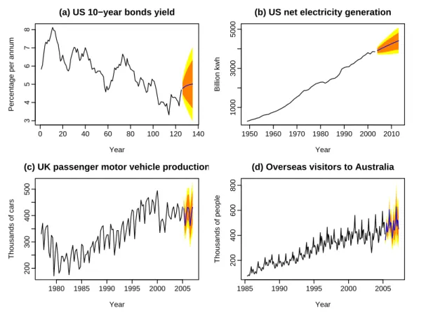
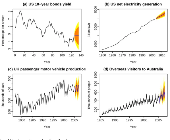
We illustrate the methods using the following four real time series shown in Figure 1. • Figure 1(a) shows 125 monthly U.S. government bond yields (percent per annum)

from January 1994 to May 2004.

• Figure 1(b) displays 55 observations of annual U.S. net electricity generation (billion kwh) for 1949 through 2003.

• Figure 1(c) presents 113 quarterly observations of passenger motor vehicle produc-tion in the U.K. (thousands of cars) for the first quarter of 1977 through the first quarter of 2005.

• Figure 1(d) shows 240 monthly observations of the number of short term overseas visitors to Australia from May 1985 to April 2005.

Figure 1:Four time series showing point forecasts and 80% & 95% prediction intervals obtained using exponential smoothing state space models.

(a) US 10−year bonds yield

Year

Percentage per annum

0 20 40 60 80 100 120 140 3 4 5 6 7 8

(b) US net electricity generation

Year Billion kwh 1950 1960 1970 1980 1990 2000 2010 1000 3000 5000

(c) UK passenger motor vehicle production

Year Thousands of cars 1980 1985 1990 1995 2000 2005 200 300 400 500

(d) Overseas visitors to Australia

Year Thousands of people 1985 1990 1995 2000 2005 200 400 600 800

(22)

3.1 Implementation of the automatic exponential smoothing algorithm

The innovations state space modelling framework described in Section 1 is implemented via the ets() function in theforecast package. For example, to apply it to the US net electricity generation time seriesuselec, we use the following commands.

etsfit <- ets(uselec) fcast <- forecast(etsfit) plot(fcast)

The object etsfitcontains all of the necessary information about the fitted model in-cluding model parameters, the value of the state vectorx_t_{for all}_t_{, residuals and so on.}

Theforecastfunction computes the required forecasts which are then plotted as in Fig-ure 1(b).

The models chosen via the algorithm were:

• ETS(A,A_d,N) for monthly US 10-year bonds yield (α = 0.99,β = 0.12,φ= 0.80,ℓ0 = 5.30,b0 = 0.71); • ETS(M,M_d,N) for annual US net electricity generation

(α = 0.99,β = 0.01,φ= 0.97,ℓ0 = 262.5,b0 = 1.12); • ETS(A,N,A) for quarterly UK motor vehicle production

(α = 0.61,γ = 0.01,ℓ0 = 343.4,s−3 = 24.99,s−2= 21.40,s−1=−44.96,s0=−1.42); • ETS(M,A,M) for monthly Australian overseas visitors

(α = 0.57, β = 0.01, γ = 0.19, ℓ0 = 86.2, b0 = 2.66, s−11 = 0.851, s−10 = 0.844,

s−9 = 0.985, s₋8 = 0.924, s₋7 = 0.822, s₋6 = 1.006, s₋5 = 1.101, s₋4 = 1.369,

s−3= 0.975,s−2= 1.078,s−1= 1.087,s0= 0.958).

Although there is a lot of computation involved, it can be handled remarkably quickly on modern computers. Each of the forecasts shown in Figure 1 took no more than a few sec-onds on a standard PC. The US electricity generation series took the longest as there are no analytical prediction intervals available for the ETS(M,M_d,N) model. Consequently, the prediction intervals for this series were computed using simulation of 5000 future sample paths.

(23)

3.2 The HoltWinters function

There is another implementation of exponential smoothing in R via theHoltWinters

function in the stats package. It implements only the (N,N), (A,N), (A,A) and (A,M) methods. The initial statesx₀ _{are fixed using a heuristic algorithm. Because of the way}

the initial states are estimated, a full three years of seasonal data is required to imple-ment the seasonal forecasts usingHoltWinters. (See Hyndman and Kostenko (2007) for the minimal sample size required.) The smoothing parameters are optimized by mini-mizing the average squared prediction errors, which is equivalent to minimini-mizing (7) in the case of additive errors.

There is apredictmethod for the resulting object which can produce point forecasts and prediction intervals. Although it is nowhere documented, it appears that the prediction intervals produced bypredictfor an object of classHoltWintersare based on an equiva-lent ARIMA model in the case of the (N,N), (A,N) and (A,A) methods, assuming additive errors. These prediction intervals are equivalent to the prediction intervals that arise from the (A,N,N), (A,A,N) and (A,A,A) state space models. For the (A,M) method, the predic-tion interval provided bypredictappears to be based on Chatfield and Yar (1991) which is an approximation to the true prediction interval arising from the (A,A,M) model. Pre-diction intervals with multiplicative errors are not possible using theHoltWinters func-tion.

3.3 Implementation of the automatic ARIMA algorithm

The algorithm of Section 2 is applied to the same four time series. Unlike the exponential smoothing algorithm, the ARIMA class of models assumes homoscedasticity which is not always appropriate. Consequently, transformations are sometimes necessary. For these four time series, we model the raw data for series (a)–(c), but the logged data for series (d). The prediction intervals are back-transformed with the point forecasts to preserve the probability coverage.

To apply this algorithm to the US net electricity generation time seriesuselec, we use the following commands.

(24)

Figure 2:Four time series showing point forecasts and 80% & 95% prediction intervals obtained using ARIMA models.

(a) US 10−year bonds yield

Year

Percentage per annum

0 20 40 60 80 100 120 140 3 4 5 6 7 8

(b) US net electricity generation

Year Billion kwh 1950 1960 1970 1980 1990 2000 2010 1000 3000 5000

(c) UK passenger motor vehicle production

Year Thousands of cars 1980 1985 1990 1995 2000 2005 200 300 400 500

(d) Overseas visitors to Australia

Year Thousands of people 1985 1990 1995 2000 2005 200 400 600 800 1000 arimafit <- auto.arima(uselec) fcast <- forecast(arimafit) plot(fcast)

The functionauto.arima()implements the algorithm of Section 2 and returns an object of classArima. The resulting forecasts are shown in Figure 2. The fitted models are as follows:

• ARIMA(0,1,1) for monthly US 10-year bonds yield (θ1 = 0.322);

• ARIMA(2,1,2) with drift for annual US net electricity generation (φ1 =−1.3031,φ2 =−0.4334,θ1 = 1.5280,θ2= 0.8338,c= 66.1473); • ARIMA(3,1,1)(2,0,1)4 model for quarterly UK motor vehicle production

(φ1 =−0.9570,φ2=−0.4500,φ3 =−0.3314,θ1 = 0.5784,Φ1 = 0.6743,Φ2 = 0.3175,

Θ1 =−0.8364;

(25)

• ARIMA(1,1,1)(2,0,0)12model with drift for monthly Australian overseas visitors (φ1 = 0.4740,θ1=−0.7393,Φ1= 0.4728,Φ2 = 0.4780,c= 0.0110).

Note that theRparameterization hasθ(B) = (1 +θ1B+· · ·+θqB)andφ(B) = (1−φ1B+ · · · −φqB), and similarly for the seasonal terms.

Theforecastpackage also contains the functionarima()which is a wrapper to the func-tion of the same name in thestatspackage. Thearima()function in theforecastpackage makes it easier to include a drift term whend+D = 1. (Settinginclude.mean=TRUEin thearima()function from thestatspackage will only work whend+D= 0.)

3.4 The forecast() function

The forecast() function is generic and has S3 methods for a wide range of time se-ries models. It computes point forecasts and prediction intervals from the time sese-ries model. Methods exist for models fitted usingets(),arima(),ar(),HoltWinters()and

StructTS().

In the latter four cases, there is also apredict()function which is intended to do much the same thing. Unfortunately, the resulting objects from thepredict function contain different information in each case and so it is not possible to build generic functions (such asplotandsummary) for the results. So, instead,forecast()acts as a wrapper to

predict(), and packages the information obtained in a common format (theforecast

class).

There is also a method for a time series object. If a time series object is passed as the first argument to forecast(), the function will produce forecasts based on the exponential smoothing algorithm of Section 1.

3.5 The forecast class

The output from theforecast()function is an object of class “forecast”. Several other functions in theforecastpackage also produce objects of this class, but they are not dis-cussed here. An object of classforecastincludes at least the following information:

• the original series;

(26)

• point forecasts;

• prediction intervals of specified coverage;

• the forecasting method used and information about the fitted model; • residuals from the fitted model;

• one-step forecasts from the fitted model for the period of the observed data.

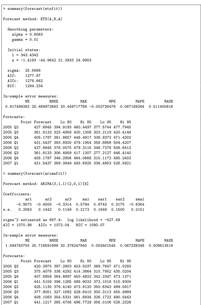
There are print, plot and summary methods for the forecast class. Figures 1 and 2 were produced using plot.forecast. Figure 3 shows the summary out-put for the forecasts plotted in Figures 1(c) and 2(c). The in-sample error mea-sures (defined in Hyndman and Koehler, 2006) for the two models are almost iden-tical. Note that the information criteria are not comparable. The prediction inter-vals are, by default, computed for 80% and 95% coverage, although other values are possible if requested. Fan charts (Wallis, 1999) are possible using the combination

plot(forecast(model.object,fan=TRUE)).

4 Comparisons

There is a widespread myth that ARIMA models are more general than exponential smoothing. This is not true. The two classes of models overlap. The linear exponen-tial smoothing models are all special cases of ARIMA models—the equivalences are dis-cussed in Hyndman et al. (2007). However, the non-linear exponential smoothing mod-els have no equivalent ARIMA counterpart. On the other hand, there are many ARIMA models which have no exponential smoothing counterpart. Thus, the two model classes overlap and are complimentary; each has its strengths and weaknesses.

The exponential smoothing state space models are all non-stationary. Models with sea-sonality or non-damped trend (or both) have two unit roots; all other models—that is, non-seasonal models with either no trend or damped trend—have one unit root. It is possible to define a stationary model with similar characteristics to exponential smooth-ing, but this is not normally done. The philosophy of exponential smoothing is that the world is non-stationary. So if a stationary model is required, ARIMA models are better. One advantage of the exponential smoothing models is that they can be non-linear. So

(27)

> summary(forecast(etsfit)) Forecast method: ETS(A,N,A)

Smoothing parameters: alpha = 0.6063 gamma = 0.01 Initial states: l = 343.4342 s = -1.4193 -44.9642 21.3933 24.9903 sigma: 25.5668 AIC: 1277.87 AICc: 1278.662 BIC: 1294.234 In-sample error measures:

ME RMSE MAE MPE MAPE MASE

0.917498382 25.469972683 20.449717769 -0.002726478 0.067189284 0.511400816 Forecasts: Point Forecast Lo 80 Hi 80 Lo 95 Hi 95 2005 Q2 427.6845 394.9193 460.4497 377.5744 477.7945 2005 Q3 361.8133 323.4959 400.1308 303.2119 420.4148 2005 Q4 405.1787 361.8657 448.4917 338.9372 471.4202 2006 Q1 431.5437 383.8920 479.1954 358.6668 504.4207 2006 Q2 427.6845 376.0575 479.3115 348.7278 506.6412 2006 Q3 361.8133 306.4959 417.1307 277.2127 446.4140 2006 Q4 405.1787 346.2906 464.0668 315.1172 495.2403 2007 Q1 431.5437 369.3949 493.6925 336.4953 526.5921 > summary(forecast(arimafit))

Forecast method: ARIMA(3,1,1)(2,0,1)[4] Coefficients:

ar1 ar2 ar3 ma1 sar1 sar2 sma1

-0.9570 -0.4500 -0.3314 0.5784 0.6743 0.3175 -0.8364 s.e. 0.2063 0.1442 0.1149 0.2173 0.1649 0.1500 0.2151 sigma^2 estimated as 667.4: log likelihood = -527.49

AIC = 1070.98 AICc = 1072.04 BIC = 1090.07 In-sample error measures:

ME RMSE MAE MPE MAPE MASE

1.584763755 25.718591689 20.378247940 0.003401545 0.067228348 0.509613519 Forecasts: Point Forecast Lo 80 Hi 80 Lo 95 Hi 95 2005 Q2 420.3970 387.2903 453.5037 369.7647 471.0293 2005 Q3 375.4078 336.4292 414.3864 315.7952 435.0204 2005 Q4 407.6859 364.8897 450.4822 342.2347 473.1371 2006 Q1 441.5159 396.1285 486.9033 372.1018 510.9300 2006 Q2 425.1130 376.4140 473.8120 350.6343 499.5917 2006 Q3 377.9051 327.1692 428.6410 300.3113 455.4989 2006 Q4 408.1083 354.5331 461.6834 326.1722 490.0443 2007 Q1 441.1217 385.4706 496.7729 356.0106 526.2328

Figure 3: Example output from thesummarymethod for theforecastclass.

(28)

time series that exhibit non-linear characteristics including heteroscedasticity may be bet-ter modelled using exponential smoothing state space models.

For seasonal data, there are many more ARIMA models than the 30 possible models in the exponential smoothing class of Section 1. It may be thought that the larger model class is advantageous. However, the results in Hyndman et al. (2002) show that the ex-ponential smoothing models performed better than the ARIMA models for the seasonal M3 competition data. (For the annual M3 data, the ARIMA models performed better.) In a discussion of these results, Hyndman (2001) speculates that the larger model space of ARIMA models actually harms forecasting performance because it introduces additional uncertainty. The smaller exponential smoothing class is sufficiently rich to capture the dynamics of almost all real business and economic time series.

(29)

References

Anderson, B. D. O. and J. B. Moore (1979) Optimal Filtering, Prentice-Hall, Englewood Cliffs.

Aoki, M. (1987)State space modeling of time series, Springer-Verlag, Berlin.

Archibald, B. C. (1990) Parameter space of the Holt-Winters’ model,International Journal of Forecasting,6, 199–229.

Assimakopoulos, V. and K. Nikolopoulos (2000) The theta model: a decomposition ap-proach to forecasting,International Journal of Forecasting,16, 521–530.

Bowerman, B. L., R. T. O’Connell and A. B. Koehler (2005) Forecasting, time series and regression: an applied approach, Thomson Brooks/Cole, Belmont CA.

Brockwell, P. J. and R. A. Davis (1991) Time series: theory and methods, Springer-Verlag, New York, 2nd ed.

Canova, F. and B. E. Hansen (1995) Are seasonal patterns constant over time? a test for seasonal stability,Journal of Business and Economic Statistics,13, 237–252.

Chatfield, C. and M. Yar (1991) Prediction intervals for multiplicative Holt-Winters, In-ternational Journal of Forecasting,7, 31–37.

Dickey, D. A. and W. A. Fuller (1981) Likelihood ratio statistics for autoregressive time series with a unit root,Econometrica,49, 1057–1071.

Durbin, J. and S. J. Koopman (2001) Time series analysis by state space methods, Oxford University Press, Oxford.

Gardner, Jr, E. S. (1985) Exponential smoothing: The state of the art,Journal of Forecasting,

4, 1–28.

Gardner, Jr, E. S. and E. McKenzie (1985) Forecasting trends in time series,Management Science,31(10), 1237–1246.

G ómez, V. (1998) Automatic model identification in the presence of missing observa-tions and outliers, Tech. rep., Ministerio de Econom´ıa y Hacienda, Direcci ón General de Análisis y Programaci ón Presupuestaria, working paper D-98009.

(30)

G ómez, V. and A. Maravall (1998) Programs TRAMO and SEATS, instructions for the users, Tech. rep., Direcci òn General de Anilisis y Programaci òn Presupuestaria, Minis-terio de Economia y Hacienda, working paper 97001.

Goodrich, R. L. (2000) The Forecast Pro methodology,International Journal of Forecasting,

16(4), 533–535.

Hannan, E. J. and J. Rissanen (1982) Recursive estimation of mixed autoregressive-moving average order,Biometrika,69(1), 81–94.

Hendry, D. F. (1997) The econometrics of macroeconomic forecasting,The Economic Jour-nal,107(444), 1330–1357.

Hylleberg, S., R. Engle, C. Granger and B. Yoo (1990) Seasonal integration and cointegra-tion,Journal of Econometrics,44, 215–238.

Hyndman, R. J. (2001) It’s time to move from ‘what’ to ‘why’—comments on the M3-competition,International Journal of Forecasting,17(4), 567–570.

Hyndman, R. J. (2007)forecast: Forecasting functions for time series, R package version 1.05.

URL:http://www.robhyndman.info/Rlibrary/forecast/

Hyndman, R. J., M. Akram and B. C. Archibald (2007) The admissible parameter space for exponential smoothing models,Annals of the Institute of Statistical Mathematics, to appear.

Hyndman, R. J., M. L. King, I. Pitrun and B. Billah (2005a) Local linear forecasts using cubic smoothing splines,Australian & New Zealand Journal of Statistics,47(1), 87–99. Hyndman, R. J. and A. B. Koehler (2006) Another look at measures of forecast accuracy,

International Journal of Forecasting,22, 679–688.

Hyndman, R. J., A. B. Koehler, J. K. Ord and R. D. Snyder (2005b) Prediction intervals for exponential smoothing using two new classes of state space models,Journal of Forecast-ing,24, 17–37.

Hyndman, R. J., A. B. Koehler, R. D. Snyder and S. Grose (2002) A state space framework for automatic forecasting using exponential smoothing methods,International Journal of Forecasting,18(3), 439–454.

(31)

Hyndman, R. J. and A. V. Kostenko (2007) Minimum sample size requirements for sea-sonal forecasting models, Foresight: the International Journal of Applied Forecasting, 6, 12–15.

Kwiatkowski, D., P. C. Phillips, P. Schmidt and Y. Shin (1992) Testing the null hypothesis of statioanrity against the alternative of a unit root,Journal of Econometrics,54, 159–178. Liu, L. M. (1989) Identification of seasonal ARIMA models using a filtering method,

Com-munications in Statistics, Part A — Theory and Methods,18, 2279–2288.

Makridakis, S., A. Anderson, R. Carbone, R. Fildes, M. Hibon, R. Lewandowski, J. New-ton, E. Parzen and R. Winkler (1982) The accuracy of extrapolation (time series) meth-ods: Results of a forecasting competition,Journal of Forecasting,1, 111–153.

Makridakis, S. and M. Hibon (2000) The M3-competition: Results, conclusions and im-plications,International Journal of Forecasting,16, 451–476.

Makridakis, S. G., S. C. Wheelwright and R. J. Hyndman (1998)Forecasting: methods and applications, John Wiley & Sons, New York, 3rd ed.

M´elard, G. and J.-M. Pasteels (2000) Automatic ARIMA modeling including intervention, using time series expert software,International Journal of Forecasting,16, 497–508. Ord, J. K., A. B. Koehler and R. D. Snyder (1997) Estimation and prediction for a class of

dynamic nonlinear statistical models,Journal of the American Statistical Association, 92, 1621–1629.

Ord, K. and S. Lowe (1996) Automatic forecasting,The American Statistician,50(1), 88–94. Pegels, C. C. (1969) Exponential forecasting: Some new variations, Management Science,

15(5), 311–315.

Reilly, D. (2000) The AUTOBOX system,International Journal of Forecasting,16(4), 531–533. Smith, J. and S. Yadav (1994) Forecasting costs incurred from unit differencing

fraction-ally integrated processes,International Journal of Forecasting,10(4), 507–514.

Taylor, J. W. (2003) Exponential smoothing with a damped multiplicative trend, Interna-tional Journal of Forecasting,19, 715–725.

Wallis, K. F. (1999) Asymmetric density forecasts of inflation and the Bank of England’s fan chart,National Institute Economic Review,167(1), 106–112.