NBER WORKING PAPER SERIES
RISK, RETURN AND DIVIDENDS Andrew Ang
Jun Liu
Working Paper 12843
http://www.nber.org/papers/w12843
NATIONAL BUREAU OF ECONOMIC RESEARCH 1050 Massachusetts Avenue
Cambridge, MA 02138 January 2007
We especially thank John Cochrane, as portions of this manuscript originated from conversations between John and the authors. We are grateful to the comments from an anonymous referee for comments that greatly improved the article. We also thank John Campbell, Joe Chen, Bob Dittmar, Chris Jones, Erik Lders, Sydney Ludvigson, Jiang Wang, Greg Willard, and seminar participants at an NBER Asset Pricing meeting, the Financial Econometrics Conference at the University of Waterloo, the Western Finance Association, Columbia University, Copenhagen Business School, ISCTE Business School (Lisbon), Laval University, LSE, Melbourne Business School, Norwegian School of Management (BI), Vanderbilt University, UCLA, UC Riverside, University of Arizona, University of Maryland, University of Michigan, UNC, University of Queensland, USC, and Vanderbilt University for helpful comments. Andrew Ang acknowledges support from the NSF. The views expressed herein are those of the author(s) and do not necessarily reflect the views of the National Bureau of Economic Research. © 2007 by Andrew Ang and Jun Liu. All rights reserved. Short sections of text, not to exceed two paragraphs, may be quoted without explicit permission provided that full credit, including © notice,
Risk, Return and Dividends Andrew Ang and Jun Liu
NBER Working Paper No. 12843 January 2007
JEL No. G12
ABSTRACT
We characterize the joint dynamics of dividends, expected returns, stochastic volatility, and prices. In particular, with a given dividend process, one of the processes of the expected return, the stock volatility, or the price-dividend ratio fully determines the other two. For example, together with dividends, the stock volatility process fully determines the dynamics of the expected return and the price-dividend ratio. By parameterizing one or more of expected returns, volatility, or prices, common empirical specifications place strong, and sometimes counter-factual, restrictions on the dynamics of the other variables. Our relations are useful for understanding the risk-return trade-off, as well as characterizing the predictability of stock returns.
Andrew Ang
Columbia Business School 3022 Broadway 805 Uris New York NY 10027 and NBER
[email protected] Jun Liu
Rady School of Management UCSD
Pepper Canyon Hall Room 320 9500 Gilman Dr MC 0093 La Jolla CA 92093
1
Introduction
Using the dividend process of a stock, we fully characterize the relations between expected returns, stock volatility, and price-dividend ratios, and derive over-identifying restrictions on the dynamics of these variables. We show that given the dividend process, one of the expected return, the stock return volatility, or the price-dividend ratio completely determines the other two. These relations are not merely technical restrictions, but they lend insight into the nature of the risk-return relation and the predictability of stock returns.
Our method of using the dividend process to characterize the risk-return relation requires no economic assumptions other than transversality to ensure that the price-dividend ratio exists and is well defined.1 In deriving our relations, we do not require the preferences of agents,
equilibrium concepts, or a pricing kernel. This is in contrast to previous work that requires equilibrium conditions, in particular, the utility function of a representative agent, to pin down the risk-return relation. For example, in a standard CAPM or Merton (1973) model, the expected return of the market is a product of the relative risk aversion coefficient of the representative agent and the variance of the market return.
The intuition behind our risk-return relations is a simple observation that, by definition, returns equal the sum of capital gain and dividend yield components. Hence, the return is determined by price-dividend ratios and dividend growth rates. In particular, if we specify the expected return process, we can compute price-dividend ratios given the dividend process. Going the other way, the price-dividend ratio, together with cashflow growth rates, can be used to infer the process for expected returns. Given the dividend process, these relations between expected returns and price-dividend ratios arise from a dynamic version of the Gordon model.
Less standard is that, given cashflows, the volatility of returns also determines price-dividend ratios and vice versa. The second moment of the return is also a function of price-dividend ratios and dividend growth rates. Thus, using dividends and price-dividend ratios, we can compute the volatility process of the stock. Going in the opposite direction, if dividends are given and we specify a process for stochastic volatility, we can back out the price-dividend ratio because the second moment of returns is determined by price-dividend ratios and dividend growth. In continuous time, we show that expected returns, stock volatility, and price-dividend ratios are linked by a series of differential equations.
Our risk-return relations are empirically relevant because our conditions impose stringent 1We use the terms dividend and cashflows interchangeably and define them to be the total payout received by a holder of an equity (stock) security.
restrictions on asset pricing models. Many common empirical applications often directly spec-ify only one of the expected return, risk, or the price-dividend ratio. Often, this is done without considering the dynamics of the other two variables. Our results show that once the cashflow process is determined, specifying the expected return automatically pins down the diffusion term of returns and vice versa. Hence, specifying one of the expected return, risk, or the price-dividend ratio makes implicit assumptions about the dynamics of these other variables. Our relations can be used as checks of internal consistency for empirical specifications that usually concentrate on only one of predictable expected returns, stochastic volatility, or price-dividend ratio dynamics. More fundamentally, the over-identifying restrictions among expected returns, volatility, and prices provide additional restrictions, even before equilibrium conditions are im-posed, on stock return predictability and the risk-return trade-off. Thus, our relations allow us to explore the implications for the joint dynamics of cashflows, expected returns, return volatility, and prices.
We illustrate several applications of our risk-return conditions with popular empirical spec-ifications from the literatures of the predictability of expected returns, time-varying volatility, and estimating the risk-return trade-off. For example, Poterba and Summers (1986) and Fama and French (1988b) estimate slow, mean-reverting components of returns. Often, empirical researchers regress returns on persistent instruments that vary over the business cycle, such as dividend yields or risk-free rates to capture these predictable components. We show that with IID dividend growth, the stochastic volatility generated by these models of mean-reverting expected returns is several orders too small in magnitude to match the time-varying volatility present in data. A second example is that many empirical studies model dividend yields, or log dividend yields as a slow, mean-reverting process. If dividend growth is IID, an AR(1) process for dividend yields surprisingly implies that the risk-return trade-off is negative. This result does not change if we allow dividend growth to be predictable and heteroskedastic, where both the conditional mean and conditional volatility are functions of the dividend yield.
Third, it is well known that volatility is more precisely estimated than first moments (see Merton, 1980). Since Engle (1982), a wide variety of ARCH or stochastic volatility models have been used to successfully capture time-varying second moments in asset prices.2 If we 2Most of the stochastic volatility literature does not consider implications of time-varying conditional volatility for expected returns. Exceptions to this are the GARCH-in-mean models that parameterize time-varying variances of an intertemporal asset pricing model. Bollerslev, Engle and Woodridge (1988), Harvey (1989), Ferson and Harvey (1991), Scruggs (1998), and Brandt and Kang (2004), among others, estimate models of this type. In contrast, most stochastic volatility models are used for derivative pricing, which only characterize the dynamics of
specify the diffusion of the stock return, then, assuming a dividend process, stock prices and expected returns are fully determined. Hence, assuming a process for the stock return volatility provides an alternative way to characterize the risk-return trade-off, rather than directly estimat-ing conditional means as a function of return volatility that is commonly done in the literature (see, for example, Glosten, Jagannathan and Runkle, 1993).
The idea of using the dividend process to characterize the relationship between risk and re-turn goes back to at least Grossman and Shiller (1981) and Shiller (1981), who argue that the volatility of stock returns is too high compared to the volatility of dividend growth. Campbell and Shiller (1988a and b) linearize the definition of returns and then iterate to derive an ap-proximate relation for the log price-dividend ratio. They use this relation to measure the role of cashflow and discount rates in the variation of price-dividend ratios by assuming that the joint dynamics are homoskedastic. Our approach is similar, in that we use the definition of returns to derive relations between risk, return, and prices. However, our relations link expected re-turns, stochastic volatility, and dividend ratios more tightly than the log-linearized price-dividend ratio formula of Campbell and Shiller. Furthermore, we are able to provide exact characterizations between the conditional second moments of returns and prices (the stochastic volatility of returns, and the conditional volatility of expected returns, dividend growth, and price-dividend ratios) that Campbell and Shiller’s framework cannot easily handle.
Our risk-return conditions are related to a series of papers that characterize the risk-return trade-off in terms of the properties of a representative agent’s utility function or the properties of the pricing kernel (see, among others, Bick, 1990; Stapleton and Subramanyam, 1990; Pham and Touzim 1996; Decamps and Lazrak, 2000; L¨uders and Franke, 2004; Mele, 2005). In particular, He and Leland (1993) show that the risk-return relation is a direct function of the curvature of the representative agent’s utility and derive a partial differential equation that the drift and diffusion term of the price process must satisfy. In contrast to these papers, we in essence use dividends, rather than preferences, to pin down the risk-return relationship. This has the advantage that dividends are observable, which allows a stochastic dividend process to be directly estimated. Indeed, a convenient assumption made by many theoretical and empirical asset pricing models is that dividend growth is IID. In comparison, there is still no consensus on the precise form that a representative agent’s utility should take.
The remainder of the paper is organized as follows. Section 2 derives the risk-return and pricing relations for an economy with an underlying variable that captures the time-varying the risk-neutral measure rather than deriving the implied expected returns of a stock under the real measure.
investment opportunity set. In Section 3, we apply these conditions to various empirical spec-ifications in the literature. Section 4 concludes. We relegate most proofs to the Appendix and some proofs are available upon request.
2
The Model
Suppose that the state of the economy is described by a single state variable xt, which follows
the diffusion process:
dxt=µx(xt)dt+σx(xt)dBxt, (1)
where the driftµx(·)and diffusionσx(·)are functions ofxt. For now, we treatxtas a scalar and
discuss the extension to a multivariatextbelow. We assume that there is a risky asset that pays
the dividend streamDt, which follows the process:
dDt Dt = µ µd(xt) + 1 2(σ 2 dx(xt) +σd2(xt)) ¶ dt+σdx(xt)dBtx+σd(xt)dBtd, (2) or equivalently: Dt D0 = exp µZ t 0 µd(xs)ds+σdx(xt)dBtx+σd(xs)dBds ¶ .
Without loss of generality, we assume thatdBtxis uncorrelated withdBtd. Note that the dividend growth process is potentially correlated withxthrough theσdxdBxt term.
By definition, the price of the assetPtis related to dividends,Dt, and expected returns,µr,
by:
Et[dPt] +Dtdt
Pt
=µrdt. (3)
By iterating equation (3), we can write the price as:
Pt= Et ·Z T t e−(Rtsµrdu)D sds+e−( RT t µrdu)PT ¸ . (4)
We show how to determine the driftµr(·)and diffusionσr(·)of the return processdRtfrom
prices and dividends:
dRt=µr(xt)dt+σr(xt)dBtr, (5)
under a transversality condition.
Assumption 2.1 The transversality condition
lim T→∞Et h e−(RtTµrdu)P T i = 0 (6)
Assumption 2.1 rules out specifications like the Black-Scholes (1973) and Merton (1973) models, which specify that the stock does not pay dividends. Equivalently, Black, Scholes, and Merton assume that the capital gain represents the entire stock return and that there are no intermediate cashflows in these economies except for the terminal capital gain of the stock. By assuming transversality, we can express the stock price in equation (4) as the value of discounted cashflows:3 Pt= Et ·Z ∞ t e−(Rtsµrdu)D sds ¸ . (7)
The following proposition characterizes the relationships between dividend growth, the drift and diffusion of the return process dRt, and price-dividend ratios, subject to the transversality
condition.
Proposition 2.1 Suppose the state of the economy is described by xt, which follows equation (1), and a stock is a claim to the dividendsDt, which follow the process in equation (2). If the price-dividend ratio Pt/Dt is a function f(·) of xt, then the cumulative stock return process,
dRt, satisfies the following equation:
dRt= µ (µx+σdxσx)f0+ 12σx2f00+ 1 f +µd+ 1 2(σ 2 dx+σ2d) ¶ dt +σx(lnf)0dBtx+σdxdBxt +σddBtd. (8) Conversely, if the returnRtsatisfies the following diffusion equation:4
dRt=µr(xt)dt+σrx(xt)dBtx+σrd(xt)dBtd, (9)
and the stock dividend process is given by equation (1), then the price-dividend ratioPt/Dt =
f(xt)satisfies the following relation:
(µx+σdxσd)f0+ 1 2σ 2 xf00− µ µr−µd− 1 2(σ 2 dx+σd2) ¶ f =−1, (10)
3An alternative way to compute the stock price is to iterate the definition of returnsdR
t= (dPt+Dtdt)/Pt forward under the transversality conditionlimT→∞exp(−(
RT t dRu− 1 2σ2rdu))PT = 0to obtain: Pt= Z ∞ t e−(Rs t dRu−12σr2du)Dsds.
This equation holds path by path. As Campbell (1993) notes, we can take conditional expectations of both the left-and right-hleft-and sides to obtain:
Pt= Et ·Z ∞ t e−(RtsdRu−12σ2rdu)Dsds ¸ ,
which can be shown to be equivalent to equation (7). 4SincedBx
t anddBtdare independent, the diffusion termσr(xt)of the return process in equation (5) is given bypσrx2 (xt) +σrd2 (xt).
and the diffusion of the stock return is determined from the relations:
σrx(x) = σx(lnf)0 (11)
σrd(x) = σd. (12)
The most important economic implication of the relations in equations (8) to (12) is that given the dividend process, specifying one of the price-dividend ratio, the expected stock re-turn, and the stock return volatility, determines the other two. In other words, suppose that the dividend cashflows are given. If we denote j ⇒ k as meaning that the process j implies the processk, then we can write:
f ⇒ µr σrx
both from equation (8).
Thus, parameterizing prices,f, determines expected returns,µrand stock return volatility,σrx.
The expected stock return alone determines both the stock price and the volatility of the return:
µr⇒ f from equation (10) σrx from equation (11),
where we solve forσrxafter solving forf. Finally, given the dividend dynamics (or thatσrdas
a function ofxis known), specifying a process for time-varying stock volatility,σrx, determines
the price of the stock and the expected return of the stock:
σrx ⇒ f from equation (11) µr from equation (10),
where the last implication for σrx ⇒ µr follows after noting that σrx determines f and f
determinesµrfrom equation (8).
Thus, with dividends specified, there is only one degree of freedom between expected re-turns, return volatility, and price-dividend ratios. More generally, if the dividend process can also be specified, then we can choose two out of the dividend, expected return, stochastic volatil-ity, and price-dividend ratio processes, with our two choices completely determining the dynam-ics of the other two variables.
In Proposition 2.1, expected returns, stochastic volatility, and dividend yields are linked to each other by a series of differential equations. Thus, by fixing a dividend process and assuming a process for one of expected returns, return volatility, or dividend yields, we may be able to
derive analytic solutions for the dynamics of the variables not explicitly modelled by working in continuous time. However, the relations in Proposition 2.1 are fundamental, and the same intuition may be obtained in discrete time, which we now discuss.
2.1
Discrete-Time Intuition
We now provide some intuition on the relations between dividends, expected returns, price-dividend ratios, and return volatility in Proposition 2.1 using a discrete-time model. From the definition of returns, we can write:
Rt+1 ≡
Pt+1+Dt+1
Pt
=µr,t+σr,tεt+1, (13)
whereµr,tis the one-period expected return,σr,t is the conditional volatility, andεt+1 is an IID
shock with unit standard deviation. To determine prices from expected returns, or vice versa, we take conditional expectations of both sides of equation (13):
Pt=
Et[Pt+1+Dt+1]
µr,t
.
We can iterate this forward to obtain a telescoping sum. Assuming transversality allows us to express the stock price as the stream of discounted cashflows:
Pt = ∞ X j=1 Et "Ãj−1 Y k=0 1 µr,t+k ! Dt+j # . (14)
Thus, knowing the cashflow series provides a mapping betweenPtand theµr,tprocess. This is
just a dynamic version of a standard Gordon dividend discount model. Hence, the basic Gordon model intuition allows us to infer prices from the expected return process, or vice versa, if dividends are given.
What is more surprising is that the volatility process determines prices, and vice versa, given the dividend series. To demonstrate this equivalence between volatility and prices in discrete time, we multiply the definition of the return byεt+1and take conditional expectations:
Et · εt+1(Pt+1+Dt+1) Pt ¸ = Et[εt+1(µt,r+σr,tεt+1)] =σr,t.
We can rearrange this expression to write the stock price in terms of conditional volatility and return innovations:
Pt=
Et[εt+1(Pt+1+Dt+1)]
σr,t
Iterating forward and assuming appropriate transversality conditions, we obtain: Pt = ∞ X j=1 Et "Ãj−1 Y k=0 εt+j+1 σr,t+j ! Dt+j # . (15)
Thus, if the dividend stream is fixed, we can invert outPtfrom theσr,tprocess, and vice versa,
in a similar fashion to inverting out prices from expected returns from the Gordon model. We can infer expected returns,µr,t, and stochastic volatility,σr,tfrom each other by equating
the price process. If expected returns are specified, then equation (14) allows us to invert a price process. Then, with a price process, we can extract the σr,t process from equation (15). Going
from σr,t to µr,t is simply the reverse procedure. Thus, with dividends specified, expected
returns, prices, and volatility of returns are all linked and knowing one process automatically pins down the other two. Thus, we obtain the same intuition in Proposition 2.1 in discrete time. In the rest of our analysis, we use continuous time, which allows us to obtain closed-form solutions.
2.2
Further Comments on the Proposition
The relations between prices, expected returns, and volatility outlined by Proposition 2.1 arise only through the definition of returns and by imposing transversality. We have not used an equilibrium model, nor do we specify a pricing kernel, to derive the relations between risk and return. The conditions (8)-(12) can be easily applied to various empirical applications because empirical models often assume a process for one or more of µr, σrx, and f. Proposition 2.1
characterizes what the functional form of the expected return, stochastic volatility, or stock price must take after choosing a parameterization of only one of these variables.
The relations between prices, expected returns, and volatility in Proposition 2.1 must hold in any equilibrium model. In an equilibrium model with a (potentially endogenous) dividend process where transversality holds, prices, returns, and volatility are simultaneously determined after specifying a complete joint distribution of state variables, agent preferences, and technolo-gies. Similarly, if a pricing kernel is specified, together with the complete dynamics of the state variables in the economy, the relations in Proposition 2.1 must also hold. Hence, the relations (8)-(12) can be viewed as necessary but not sufficient conditions for equilibrium asset pricing models.
The major advantage of the set-up of Proposition 2.1 over an equilibrium framework is that many empirical specifications in finance parameterize the conditional mean or variance of
returns (for example, predictability regressions that specify the conditional mean or stochastic volatility models), without specifying a full underlying equilibrium model. In these situations, Proposition 2.1 implicitly pins down the other characteristics of returns and prices that are not explicitly assumed. In a proof available upon request, we show that an empirical specification of a particular conditional mean, variance or a price process does not necessarily uniquely determine a pricing kernel. This is especially useful for an empirical researcher who can write down a particular expected return or volatility process knowing that there exists at least one (and potentially an infinite number of) pricing kernels that can support the researcher’s choice of the expected return or volatility process.
In Proposition 2.1, there are two effects if we relax the assumption of transversality. First, the transversality Assumption 2.1 ensures that the price-dividend ratio is a function of x by Feynman-Kacs. The requirement that Pt/Dt = f(xt) is not satisfied in economies that only
assume geometric Brownian motion processes for the stock process and do not specify cashflow components (like Black and Scholes, 1973; Merton, 1973). In these economies, there is also no state variable describing time-varying investment opportunities as the mean and variance are constant. Second, if we relax the transversality condition, the ordinary differential equation defining the price-dividend ratio in equation (10) may have additional terms with derivatives with respect to timet, and an additional boundary condition. This is due to the fact that when transversality does not hold, the price-dividend ratio is also potentially a function of timet.
Proposition 2.1 also applies to total returns, rather than excess returns. While some em-pirical studies focus on matching the predictability of total returns (see, for example, Fama and French, 1988a,b; Campbell and Shiller, 1988a) and the volatility of total returns (see, for example, Lo and MacKinlay, 1988), we often build economic models to explain time-varying excess returns, rather than total returns. Time-varying total returns may be partially driven by stochastic risk-free rates. Short rates could be included as a state variable inxt, especially since
Ang and Bekaert (2006) and Campbell and Yogo (2006), among others, find risk-free rates have predictive power for forecasting excess returns. In Section 3, we explicitly investigate the implications of a system where risk-free rates linearly predict excess returns. An alternative way to handle excess returns is to adjust Proposition 2.1 to solve for conditional excess returns, since the nominal risk-free rate is known at time tover various horizons. Note that with daily or weekly returns, there is negligible difference between total and excess returns.
Finally, although Proposition 2.1 is stated for a univariate state variable xt, the equations
ordinary differential equation (10) becomes a partial differential equation, whereµx,σx,µd,σd,
σrx, and σrd represent matrix functions of x. An integrability condition is required to ensure
that the pricing function is well-defined. This allows the vector of diffusion terms of the return process to imply a price-dividend ratio and an expected return process that are unique up to an integration constant. A proof of the multivariate case is available upon request.
3
Empirical Applications
Proposition 2.1 can be used to characterize the joint dynamics of expected returns (µr), return
volatility (σr) dividend yields (D/P) or price-dividend ratios, and dividend growth, (dD/D).
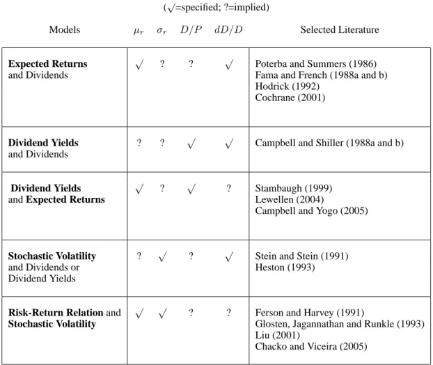
In Table 1, we provide a brief summary of various model specifications in the finance literature. We list some possible model specifications betweenµr, σr, D/P, anddD/Din each row and
if a particular model specifies the dynamics of one of these four variables, we denote which variable is specified by bold font in the first column. The “√” marks in the second column denote which of these four variables are specified, while the “?” marks denote the variables whose dynamics are implied by parameterizing the other two variables. The third column lists selected papers that assume a model for the variable in bold font.
For example, in the first row of Table 1, Fama and French (1988a and b), Hodrick (1992), Poterba and Summers (1986), and Cochrane (1991) are examples of studies which parameterize the expected return process. These authors assume that expected returns are a linear function of dividend yields, whereas Poterba and Summers assume a slow mean-reverting process for expected returns. If a dividend process is also assumed together with a model for expected returns, then the dynamics of stock volatility (σr) and dividend yields (D/P) are completely
determined by the expected return and dividend growth processes. Another example is the fourth row, where a large literature assumes a process for stochastic volatility (see, among others, Stein and Stein, 1991; Heston, 1993). Combined with an assumption on dividends, Proposition 2.1 completely determines the risk-return trade-off and prices.
Our goal in this section is to illustrate how Proposition 2.1 can be applied to various em-pirical models that have been specified in the literature. Investigating the joint dynamics of expected returns, volatility, prices, and dividends produces sharper predictions of risk-return trade-offs, expected return predictability and delivers strong pricing implications. We work mainly with the assumption that dividends are IID, which is made in many exchange-based economic models. Many economic frameworks advocate IID dividend growth, including the
textbook expositions by Campbell, Lo and MacKinlay (1997) and Cochrane (2001). Follow-ing this literature, in many of our examples, we make the assumption of IID dividend growth for illustrative purposes. This also highlights the non-linearities induced by the present value relation without specifying additional non-linear dynamics in the cashflow process. Neverthe-less, we also examine a system where dividend growth is predictable and heteroskedastic. We also examine features of the dividend growth process implied by common specifications of the expected return and stochastic volatility processes.
In Section 3.1, we briefly confirm that Proposition 2.1 nests the special Shiller (1981) case of constant expected returns, IID dividend growth, and constant price-dividend ratios. Section 3.2 analyzes the case of specifying expected returns and dividend growth by focusing on a sys-tem where the risk-free rate can predict excess returns. In Section 3.3, we consider a common mean-reverting specification for dividend yields combined with IID dividend growth or divi-dend growth that is predictable and heteroskedastic. Section 3.4 investigates the implications of the Stambaugh (1999) model for dividend growth and the risk-return trade-off, while Section 3.5 examines the implications for expected returns from various models of stochastic volatility. Finally, we parameterize the risk-return trade-off and stochastic volatility in Section 3.6.
3.1
IID Dividend Growth
If dividend growth is IID, then varying price-dividend ratios can result only from varying expected returns. The following corollary shows that under IID dividend growth, time-varying expected returns, price-dividend ratios, and time-time-varying volatility are different ways of viewing a predictable state variable driving the set of investment opportunities in the economy.
Corollary 3.1 Suppose that dividend growth is IID, so thatµd= ¯µdandσd = ¯σdare constant in equation (2). If the state variable describing the economy satisfies equation (1) and stock returns are described by the diffusion process in equation (9), whereσrd = ¯σrd is a constant, then the following statements are equivalent:
1. The price-dividend ratiof = ¯f is constant. 2. The expected returnµr= ¯µris constant.
3. The volatility of stock returns is the same as the volatility of dividend growth, orσrx = 0 in equation (9).
We can interpret the termσrx in equation (9) as the excess volatility of returns that is not
due to fundamental cashflow risk. Shiller (1981) argues that the volatility of stock returns is too high compared to the volatility of dividend growth in an environment with constant expected returns. Cochrane (2001) provides a pedagogical discussion of this issue and claims that excess volatility is equivalent to price-dividend variability, if cashflows are not predictable. Corollary 3.1 is the mathematical statement of this claim.
3.2
Specifying Expected Returns and Dividends
In an environment where the price-dividend ratio is stationary, time-varying price-dividend ra-tios must reflect variation in either discount rates or cashflows, or both. If dividend growth is IID, then the only source of time variation for price-dividend ratios is discount rates. We investigate two parameterizations of the expected return process while assuming that dividend growth is IID. First, we assume that expected returns are linear functions of dividend yields. Second, we assume that the expected stock return is a mean-reverting function of a predictable state variable, which we specify to be the risk-free rate.
3.2.1 Dividend Yields Linearly Predicting Returns
A large number of empirical researchers find that stock returns can be predicted by price-dividend ratios or price-dividend yields in linear regressions.5 The following corollary investigates the effect of linear predictability of returns by log dividend yields on the price process:
Corollary 3.2 Assume that dividend growth is IID, so µd = ¯µd andσd = ¯σd are constant in equation (2) and that σdx = 0. Suppose that the log dividend yieldln(D/P)linearly predicts returns in the predictive regression:
dRt= (α+βxt)dt+ ¯σrx(xt)dBtx+ ¯σddBtd, (16)
where the predictive instrumentx=−lnf is the log dividend yield andσ¯rxis a constant. Then, the dividend yieldxfollows the diffusion:
dxt=µx(xt)dt+σx(xt)dBxt, (17)
5Papers examining the predictability of aggregate stock returns by dividend yields include Fama and French (1988), Campbell and Shiller (1988a and b), Hodrick (1992), Goetzmann and Jorion (1993), Stambaugh (1999), Engstrom (2003), Goyal and Welch (2003), Valkanov (2003), Lewellen (2004), Ang and Bekaert (2006), and Campbell and Yogo (2006).
where the driftµx and diffusionσxare given by: µx(x) = ¯µd+ 1 2σ¯ 2 d+ 1 2σ¯ 2 rx−α−βx+ex σx(x) = −¯σrx. (18)
In Corollary 3.2 implies the sign of σx is negative, indicating that shocks to returns and
log dividend yields are conditionally negatively correlated. Since the relative volatility of log dividend shocks (σd) is small compared to the total variance of returns, the negative conditional
correlation of returns and log dividend yields is large in magnitude. This is true in the data: Stambaugh (1999) reports that the conditional correlation between level dividend yield innova-tions and innovainnova-tions in returns is around -0.9 for U.S. returns, and Ang (2002) reports a similar number for the correlation between shocks to log dividend yields and returns. Note that log dividend yields predicting returns makes the strong (counter-factual) prediction that returns are homoskedastic.
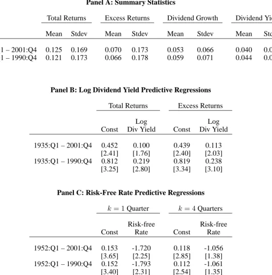
We calibrate the resulting log dividend yield process by estimating the regression implied from the predictive relation (16). We use aggregate S&P500 market data at a quarterly fre-quency from 1935 to 2001. In Panel A of Table 2, we report summary statistics of log stock returns, both total stock returns and stock returns in excess of the risk-free rate (3-month T-bills), together with dividend growth and dividend yields. From Panel A, we set the mean of dividend growth at µ¯d = 0.05and dividend growth volatility at σ¯d = 0.07. The volatility of
dividend growth is much smaller than the volatility of total returns and excess returns, which are very similar, at approximately 18% per annum. This allows us to setσ¯rx2 = (0.18)2 −(0.07)2, or¯σrx = 0.15. Empirically, the correlation between dividend growth and total or excess returns
is close to zero (both correlations being around -0.08). This justifies our assumption in setting
σdx = 0.
In Panel B of Table 2, we report linear predictability regressions of continuously com-pounded returns over the next year on a constant and log dividend yields. Since the data is at a quarterly frequency, but the regression is run with a 1-year horizon on the left-hand side, the regression entails the use of overlapping observations that induces moving average error terms in the residuals. We report Hodrick (1992) standard errors in parentheses, which Ang and Bekaert (2006) show to have good small sample properties with the correct empirical size. Goyal and Welch (2003), among others, document that dividend yield predictability declined substantially during the 1990s, so we also report results for a data sample that ends in 1990.
The coefficients in the total return regressions are similar to the regressions using excess returns. For example, over the whole sample, the coefficient for the log dividend yield is 0.10
using total returns, compared to 0.11 using excess returns. Hence, although we perform our calibrations for total returns, similar conditional relations also hold for excess returns. The second line of Panel B shows that when the 1990s are removed from the sample, the magnitude of the predictive coefficients increases by a factor of approximately two. To emphasize the linear predictive relationship in equation (16), we focus on calibrations using the sample without the 1990s. Nevertheless, we obtain similar qualitative patterns for the implied functional form for the drift of the price process when we calibrate parameter values using data over the whole sample.
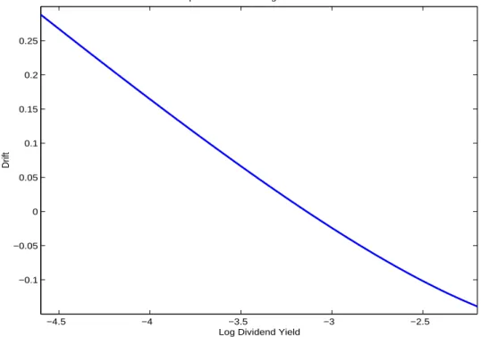
Since the predictive regressions are run at an annual frequency, the estimated coefficients in Panel B allow us to directly match α and β, since we can discretize the drift in equation (16) as approximately (α+βx)∆t. Hence, we setα = 0.81andβ = 0.22. Together with the calibrated values forµ¯d= 0.05,σ¯d= 0.07andσ¯rx = 0.15, we compute the implied drift of the
log dividend yield using equation (18). Figure 1 plots the drift of the log dividend yield, which shows it to be almost linear. Hence, if log dividend yields predict returns and dividend growth is IID, then linear approximations for log dividend yields will be very accurate.6 This implies that
log-linearized systems like Campbell and Shiller (1988a,b) contain little approximation error for the dynamics of the log dividend yield.
3.2.2 Predictable Mean-Reverting Components of Returns
As a second example of specifying an expected return process, we assume that excess returns are predictable by risk-free rates.7 Ang and Bekaert (2006) find that the strength of the pre-dictability of excess returns by risk-free rates is much stronger at short horizons than dividend yields, which is confirmed by Campbell and Yogo (2006). Denoting the risk-free rate asx, we consider the following system where the risk-free rate predicts excess returns:
dRt = (xt+α+βxt)dt+σrx(xt)dBtx+ ¯σddBtd, (19)
where the short ratexfollows the Ornstein-Uhlenbeck process:
dxt=−κ(xt−θ)dt+ ¯σxdBt+ ¯σxddBtd (20)
6If we model the level dividend yield as predicting returns in equation (16) similar to Fama and French (1988a), then the implied drift of the level dividend yield is highly non-linear, becoming strongly mean-reverting at high levels of the dividend yield, but behaves like a random walk at low dividend yield levels.
7Papers examining predictability of stock returns by risk-free rates include Fama and Schwert (1977), Campbell (1987), Lee (1992), Ang and Bekaert (2006), and Campbell and Yogo (2006).
These equations imply that the term structure is a Vasicek (1977) model and that the excess stock return is predicted by the short rate. The set-up also allows dividend growth and risk-free rates to be correlated through theσ¯xdparameter.
In Panel C of Table 2, we report coefficients of predictive regressions for excess returns over a 1-quarter and a 4-quarter horizon. We use annualized, continuously compounded 3-month T-bill rates as the predictive variable over the post-1952 sample because interest rates were pegged by the Federal Reserve prior to the 1951 Treasury Accord. The results confirm Ang and Bekaert’s (2006) findings that the predictive power of the risk-free rate is best visible at short horizons, where the coefficient on the risk-free rate is -1.72 with a robust t-statistic of 2.25. Risk-free rate predictability is slightly stronger in the sample ending in 1990, where the predictive coefficient is -1.79 with a t-statistic of 2.31. At a 4-quarter horizon, the risk-free coefficients drop to around -1.06 for both samples and are no longer significant at the 5% level. For our calibrations, we use the regression coefficients from the 1952-2001 sample at a quarterly horizon, giving us values of α = 0.15and β = −1.72. The unconditional mean of short rates over this sample isθ = 0.053. We also match the annual risk-free rate autocorrelation of0.787 = exp(−κ), the unconditional risk-free rate volatility of0.0275, and the correlation of risk-free rates and dividend growth of 0.214 in the data. Thus,σ¯xandσ¯xdsatisfy
(0.0275)2 = ¯σ 2 x+ ¯σxd2 2κ and 0.214 = ¯ σxd ¯ σxσ¯d .
We also assume that the mean of dividend growth and the volatility of dividend growth are constant atµ¯d = 0.05andσ¯d = 0.07, respectively.
Our goal is to characterize the behavior of price-dividend ratios and the implied stochastic volatility induced by the predictability of the excess return by risk-free rates. We can solve for price-dividend ratios exactly using equation (7) to obtain:
Pt Dt = Et ·Z ∞ t exp µ − Z s t (xu+α+βxu)du ¶ exp¡µ¯d(s−t) + ¯σd(Bsd−Btd) ¢¸ ds = Z ∞ t exp µ − µ α−µ¯d− 1 2σ¯ 2 d ¶ (s−t) ¶ ×Et · exp µ − Z s t (1 +β)xudu ¶ exp µ −1 2σ¯ 2 d(s−t) + ¯σd(Bsd−Btd) ¶¸ ds = Z ∞ t exp µ − µ α−µ¯d− 1 2σ¯ 2 d ¶ (s−t) ¶ EQt · exp µ − Z s t (1 +β)xudu ¶¸ ds,
where the measureQis determined by its Radon-Nikodym derivative with respect to the original measure exp µZ ¯ σddBtd− 1 2σ¯ 2 ddt ¶ .
By Girsanov’s theorem, the dynamics of the short ratexunderQis:
dxt =−κ(xt−θ−σ¯dσ¯xd/κ)dt+ ¯σxdBt+ ¯σxddBtQd.
Hence, we can write the price-dividend ratio as:
Pt Dt = Z ∞ t exp µ − µ (1 +β) ³ θ+ σ¯dσ¯xd κ ´ +α−µ¯d− 1 2σ¯d ¶ s −(1 +β) ³ xt−θ− ¯ σd¯σxd κ ´1−e−κs κ +(¯σ 2 x+ ¯σ2xd)(1 +β)2 2κ2 µ s− 2(1−e −κs) κ + 1−e−2κs 2κ ¶¶ ds. (21)
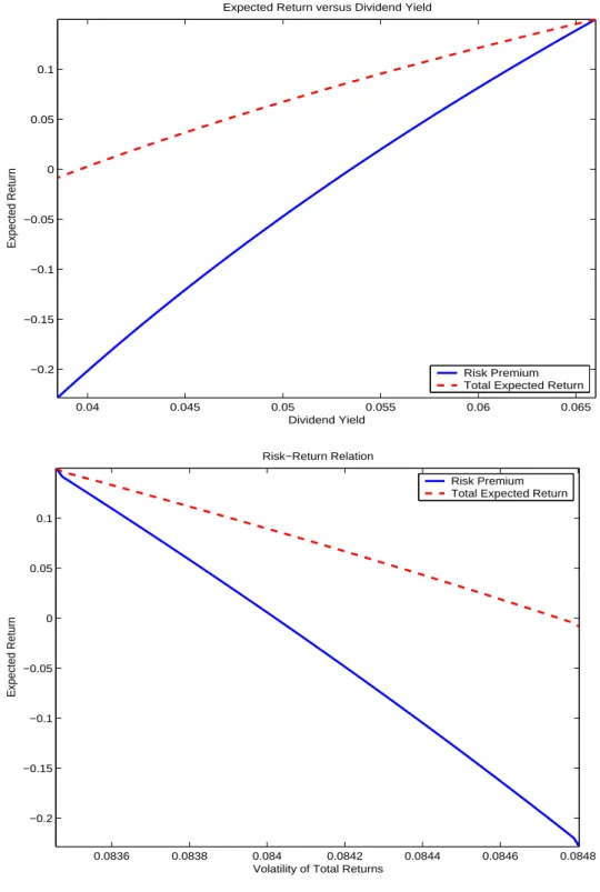
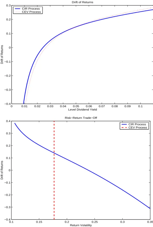
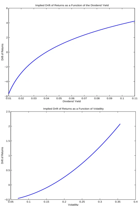
In the top panel of Figure 2, we graph the risk premium, α+βx, and the total expected return,x+ (α+βx), as a function of the dividend yield. The top panel of Figure 2 shows that the expected return is a strictly increasing, convex function of the dividend yield. Thus, high dividend yields forecast high expected total and excess returns. The bottom panel of Figure 2 plots the implied risk-return trade-off of the excess return predictability system. We plot the risk premium and total expected returns against σr =
p
σ2
rx(x) +σ2d. There are two notable
features of this bottom plot.
First, the range of the implied volatility of returns is surprisingly small, not showing much variation around 0.084, which is not much different to the volatility of dividend growth at 0.07. The implied volatility is also much smaller than the standard deviation of returns in data, which is around 0.18. The intuition behind this result is that large changes in the price-dividend ratio,
f, are required to produce a large amount of stochastic volatility through the relation σrx =
¯
σx(lnf)0 in equation (11) of Proposition 2.1. When expected returns are mean-reverting, only
the terms in the sum (7) close to t change dramatically when x changes. One way for small changes inxto induce large changes inf is for the predictive coefficient to be extremely large in magnitude, but this causes total expected returns to be unconditionally negative. We can also generate larger amounts of heteroskedasticity if the mean reversion coefficient in the predictive variable, κ, is close to zero, which corresponds to the case of permanent changes in expected returns.
Second, the risk-return relation in Figure 2 is downward sloping, so that high volatility coincides with low risk premia. This is due to the convexity imbedded in the present value relation. When expected returns are low, price-dividend ratios are high. A standard duration argument implies that there are relatively large price movements resulting from small changes in expected returns at high price levels and relatively small price movements resulting from small
changes in expected returns at low price levels. Hence, the risk-return relation is downward sloping. This result suggests that we may need an additional volatility factor to explain the amount of heteroskedasticity present in stock returns. Alternatively, heteroskedastic dividend growth may change the shape of the risk-return trade-off, which we examine in the next section.
3.3
Specifying Dividend Yields and Dividends
Many studies, like Stambaugh (1999), Lewellen (2004), and Campbell and Yogo (2005) specify the dividend yield to be a mean-reverting process. We now investigate the implied dynamics of expected returns and the risk-return trade-off implied by mean-reverting dividend yields. Our first case uses IID dividend growth, while our second example considers predictable and heteroskedastic dividend growth.
3.3.1 IID Dividend Growth
Corollary 3.3 Assume that dividend growth is IID, so µd = ¯µd andσd = ¯σd are constant in equation (2), and thatσdx= 0. Suppose that the level dividend yieldx= 1/f, wheref =P/D, follows the CEV process:
dxt=κ(θ−xt)dt+σxγtdBxt. (22)
Then, the driftµr and diffusionσrx of the return processdRtin equation (9) satisfy:
µr(x) = κ+ ¯µd+ 1 2σ¯ 2 d− κθ x +σ 2x2(γ−1)+x σrx(x) = −σxγ−1 (23)
If dividend yields are mean-reverting, Corollary 3.3 shows that returns are heteroskedastic, asσrx =−σxγ−1. For the special case of a Cox, Ingersoll and Ross (1987) (CIR) process where
γ = 0.5, high dividend yieldsxtend to coincide with low return volatility, since in this special case σrx = −σx/
√
x. This is the opposite to the behavior of these variables in data because during recessions or periods of market distress, dividend yields tend to be high and stock returns tend to be volatile. For a CEV process withγ = 1, Corollary 3.3 states that the return volatility must be constant, even though expected returns are time-varying.
We calibrate the parameters κ, θ, and σ in equation (22) to match the moments of the dividend yield. We match the quarterly autocorrelation,0.96 = exp(−κ/4); the unconditional mean θ = 0.044; and the unconditional variance (0.0132)2 = σ2θ/(2κ) for a CIR process. For a CEV process withγ = 1, we also calibrateσby matching the unconditional variance of
dividend yields, using the relation (0.0132)2 = σ2θ2/(2κ−σ2). Dividend growth has a low correlation with dividend yields, at 0.05 in data, so the assumption thatσdx = 0is realistic.
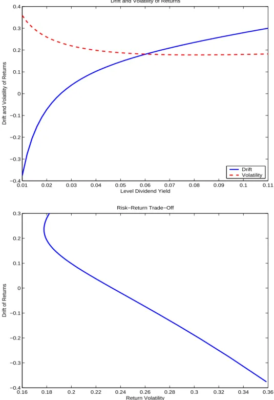
We characterize the behavior of expected returns and the risk-return trade-off implied by mean-reverting dividend yields in Figure 3. The top panel graphs the drift of returns as a mono-tonic, increasing function of dividend yields. Both the cases where dividend yields follow a CIR process or a CEV process withγ = 1produce very similar drift functions. However, Corollary 3.3 shows that expected returns may not always be monotonically increasing functions of the dividend yield. For example, if dividend yields follow a CIR process, thenµr is given by:
µr(x) = κ+ ¯µd+ 1 2σ¯ 2 d− κθ−σ2 x +x,
which may increase steeply as dividend yieldsxapproach zero ifκθ > σ2.
While low dividend yields do not coincide with high expected returns for the parameter values calibrated to data, Corollary 3.3 shows that low dividend yields may forecast high returns in well-defined dynamic economies. To provide some intuition behind this result, we use the definition of a discrete-time expected return:
µr,t = Et[Pt+1] Pt +Et[Dt+1] Pt .
In a one-period model (or in a setting wherePt+1 = 0),µr,t = Et[Dt+1]/Pt, so low prices imply
high expected returns. However, givenEt[Dt+1]in a multi-period setting, lowPtcan imply low
µr,tif: (i) low prices today imply low conditional prices next period, or (ii) low prices imply a
large positive Jensen’s term. The former does not occur if dividend yields are mean-reverting, but large Jensen’s terms may arise in practice (see, for example, P´astor and Veronesi, 2006).
The bottom panel of Figure 3 plots the risk-return relation implied by mean-reverting divi-dend yields and IID dividivi-dend growth. The risk-return relation is strongly downward sloping if dividend yields follow a CIR process. For a CEV process withγ = 1, the risk-return relation is degenerate because the implied return volatility is constant.8 Reasonable economic models
usually imply that the risk premium is a weakly, or strictly, increasing function of volatility, so downward sloping risk and total expected return relations could arise if the risk-free rate de-creases faster than the risk premium inde-creases when volatility rises. Without this effect, a much less restrictive conditional mean µx(·) is required in equation (22), rather than the standard
8In the case where the log dividend yieldx=−lnffollows an AR(1) process and dividend growth is IID (see Corollary 3.2), the risk-return relation is also degenerate because the return volatility is constant while expected returns vary over time.
AR(1)κ(θ−x)formulation, to order for the risk-return trade-off to be positive when dividend growth is IID.
3.3.2 Predictable and Heteroskedastic Dividend Growth
A number of recent studies suggest that dividend growth is predictable (see Bansal and Yaron, 2004; Hansen, Heaton and Li, 2005; Lettau and Ludvigson, 2005; Ang and Bekaert, 2006) and that dividend growth exhibits significant heteroskedasticity (see Calvet and Fisher, 2005). In this section, we examine the implied risk-return trade-off for a system where dividend yields are mean-reverting but dividend growth exhibits predictable and heteroskedastic components which are functions of the dividend yield.
Corollary 3.4 Assume that the level dividend yieldx= 1/f, wheref =P/D, follows the CIR process:
dxt=κ(θ−xt)dt+σ
√
xtdBtx, (24)
and that the log dividend level follows the process: dlnDt= (α+βxt)dt+b
√
xtBtd, (25)
where the correlation between dBtx andBtdis zero. Then, the driftµr and diffusionσrx of the return processdRtin equation (9) satisfy:
µr(x) = κ+α+ (σ2−κθ) x + µ 1 +β+1 2b 2 ¶ x σrx(x) = − σ √ x (26)
In Corollary 3.4, the level dividend yield is mean-reverting but is constrained to be positive through the square-root process. In equation (25), dividend growth is predictable by the divi-dend yield, which is what Ang and Bekaert (2006) find. The conditional volatility of dividivi-dend growth increases as the dividend yield increases. This is economically reasonable, as during periods of market distress, dividend yields are high because prices are low, and there is larger uncertainty about future cashflows.
To match the dynamics of the dividend yield, we setκ= 0.16,θ= 0.044, andσ = 0.0365to match the autocorrelation, mean and variance of the dividend yield. To calibrate the conditional mean of log dividend processes in Corollary 3.4, we regress annualized quarterly dividend growth onto the dividend yield:
where gt+1 = ln(Dt+1/Dt) is quarterly dividend growth, anddyt is the level dividend yield.
Over the 1952-2001 sample,α= 0.026andβ = 0.415, with robust t-statistics of 2.63 and 3.70, respectively. This result is consistent with the positive OLS coefficients for the dividend yield predicting dividend growth reported by Ang and Bekaert (2006).
It can be shown that the unconditional variance of dividend growth fors > tis given by:
E[(lnDs−lnDt−E[lnDs−lnDt])2] = Ã b2+ µ βσ κ ¶2! (s−t)θ− β2σ2 κ3 (1−e −κ(s−t))θ.
This formula for s−t = 1 allows us to match the unconditional variance of annual dividend growth. The volatility of annualized dividend growth,gt,t+4 =gt+1+gt+2+gt+3+gt+4, is 0.0932
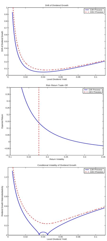
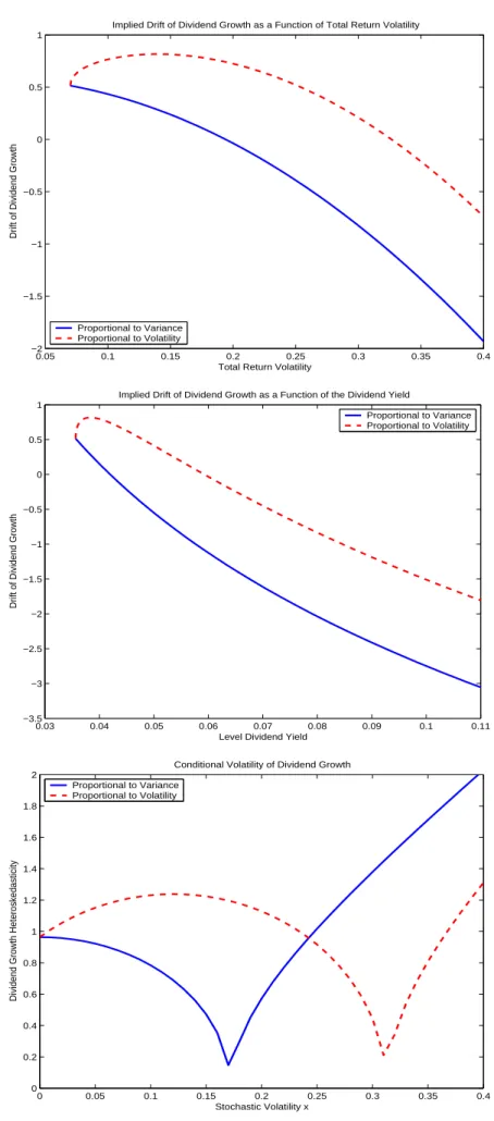
in data, which is matched by a value ofb = 0.444. As expected from equations (24) and (25), the unconditional correlation between dividend growth and dividend yields is controlled by the parameter β. In data, the correlation between annual dividend growth and dividend yields is 0.16, which is only slightly larger than the correlation implied by the model parameters at 0.06. In the top panel of Figure 4, we plot the drift and volatility of returns implied by predictable and heteroskedastic dividend growth (equation (26)). In the solid line, the expected return assumes a concave shape which increases with the dividend yield. For the return volatility in the dashed line, we plotpσrx2 +σ2rdas a function of the dividend yield,x, where σrd = b
√
x. The volatility of returns is highest when dividend yields are low (or prices are high). This implication seems to be counter-factual as stock return volatility increases during periods of market distress when prices are low and dividend yields are high. However, the conditional volatility curve is slightly U-shaped and increases also when dividend yields are high.
The bottom panel plots the implied risk-return trade-off. First, the risk-return trade-off does not have a unique one-to-one correspondence. This is due to the U-shape pattern of return volatility increasing at high dividend yields. Thus, according to this specification for dividend cashflows, the risk-return trade-off will be particularly difficult to pin down for low to moderate return volatility levels. However, the general shape of the risk-return trade-off is downward sloping, similar to the IID dividend growth case in Figure 3. Thus, either considerably more heteroskedasticity in dividends is needed, or a richer non-linear specification for the dividend yield is required to generate an upward sloping risk-return relation.
3.4
Specifying Dividend Yields and Expected Returns
We take the Stambaugh (1999) model as a well-known example of a system that specifies the joint dynamics of dividend yields and expected returns. Stambaugh assumes that the dividend yield x = D/P follows an AR(1) process and that the stock return is a linear function of the dividend yield. We modify the Stambaugh system slightly to use a CIR process or a CEV process with to ensure that prices are always positive. Hence, the Stambaugh model specifies:
dRt = (α+βxt)dt+σrx(xt)dBtx+σd(xt)dBtd
dxt = κ(θ−xt)dt+σxγtdBtx, (27)
wherexis the dividend yield,x=D/P, withγ = 0.5(γ = 1.0) for a CIR (CEV) dividend yield process. Stambaugh uses this system to assess the small sample bias in a predictive regression where the dividend yield is an endogenous regressor. By jointly specifying dividend yields and expected returns, Stambaugh implicitly implies the dynamics of dividend growth and the risk-return trade-off.
A further application of Proposition 2.1 implies that the drift ofdDt/Dtin equation (2) can
be written as a function of the dividend yieldx:
µd(x) + 1 2σ 2 d(x) =α−κ+ (β−1)x+ κθ x −σ 2 xx2(γ−1), (28)
assuming that σxd = 0, which is true empirically. Hence, by assuming that dividend yields are
mean-reverting and that dividend yields monotonically predict expected returns, Proposition 2.1 implies that dividend yields must predict dividend growth.
We graph equation (28) in the top panel of Figure 5, which shows that dividend growth is a highly non-monotonic function of dividend yields. For very low dividend yields, dividend growth is a decreasing function of dividend yields. However, for dividend yields above 3%, dividend growth is an increasing function of dividend yields. Since empirically dividend yields have only been below 2% for a short episode during the late 1990s, we should expect that, on average, dividend yields should positively predict dividend growth. This result is the opposite to the intuition of Campbell and Shiller (1988a,b) who claim that high dividend yields must forecast either high future returns or low future dividends.9
9If we model dividend yields,D/P = x, in equation (27) to be an AR(1) process, then the drift of dividend growth takes on a concave shape as a function of the dividend yield, which decreases to−∞as the level dividend yield approaches zero from the right-hand side.
To provide some discrete-time intuition on this result, we use the definition of expected returns to write: µr,t= Et · Pt+1+Dt+1 Pt ¸ = Dt Pt µ Et · 1 Dt+1/Pt+1 ¸ + 1 ¶ Et · Dt+1 Dt ¸ .
Given the expected return,µr,t, in a multi-period model, highDt/Ptimplies a highEt[Dt+1/Dt]
if high dividend yields cause a large Jensen’s term or high dividend yields forecast high dividend yields next period. The latter result cannot occur if dividend yields are mean-reverting. In contrast, in a one-period setting (or wherePt+1 = 0), high dividend yields forecast low dividend
growth for a given expected return,µr,t:
µr,t = Dt Pt Et · Dt+1 Dt ¸ .
Hence, the result that dividend yields positively forecast future dividend growth can occur only in a dynamic model.
The middle panel of Figure 5 plots the return-risk trade-off implied by the Stambaugh model. If we assume that dividend growth is homoskedastic and set σ¯d = 0.07, we can
in-vestigate the risk-return trade-off implied by the (α +βx) expected return assumption in the drift of the stock return and the volatility of the stock return,σr =
p
σ2
rx+ ¯σ2d. Since the
divi-dend yield is mean-reverting according to equation (27) in the Stambaugh system, the diffusion term of the return process takes the form σrx(x) = −σxγ−1, similar to equation (23). Figure
5 shows that the risk-return trade-off is monotonically downward sloping for a CIR dividend yield process and the return volatility is constant if dividend yields follow a CEV process. We can induce a positive risk-return trade-off only by relaxing the assumption that dividend yields non-monotonically predict expected returns, rather than the linear(α+βx)drift term in equa-tion (27), or by assuming a richer condiequa-tional mean specificaequa-tion for the dynamics of dividend yields.
Finally, we consider the implied behavior of dividend growth heteroskedasticity from the Stambaugh model. Following Calvet and Fisher (2005), we set the conditional mean of div-idend growth to be constant, at µ¯d = 0.05, but solve endogenously for dividend growth
het-eroskedasticity. Using equation (28), we plot the conditional volatility of dividend growth,|σd|
as a function of the level dividend yield in the bottom panel of Figure 5. Interestingly, the implied volatility of dividend growth is a non-monotonic function of the dividend yield and increases in periods of both low and high dividend yields, which would roughly correspond to the peaks and troughs of business cycle variation. A multi-frequency model of dividend growth
heteroskedasticity, like Calvet and Fisher, where shocks to dividend growth occur jointly over different frequencies, could potentially match this pattern.
3.5
Specifying Stochastic Volatility and Dividends
The dynamics of time-varying variances of stock returns have been successfully captured by a number of models of stochastic volatility. If the dividend process is specified, Proposition 2.1 shows that the presence of stochastic volatility implies that stock returns must be predictable. We now use Proposition 2.1 to characterize stock return predictability by parameterizing the variance process. Thus, Proposition 2.1 can be used to shed light on the nature of the aggregate risk-return relation, on which there is no theoretical or empirical consensus. This is an entirely different approach from the current approach in the literature of estimating the risk-return trade-off, which uses different measures of conditional volatility in predictive regressions to estimate the conditional mean of stock returns (see, for example, Glosten, Jagannathan and Runkle, 1996; Scruggs, 1998; Ghysels, Santa-Clara and Valkanov, 2005).
We look at two well-known stochastic volatility models, the Gaussian model of Stein and Stein (1991) in Section 3.5.1 and the square root model of Heston (1993) in Section 3.5.2.10
In both cases, we assume that dividend growth is IID (µd = ¯µd and σd = ¯σd are constant in
equation (2)), and setσdx = 0to focus on the relations between risk and return induced by the
non-linear present value relation.
3.5.1 The Stein-Stein (1991) Model
In the Stein and Stein (1991) model, time-varying stock volatility is parameterized to be an Ornstein-Uhlenbeck process. The Stein-Stein model in our set-up can be written as:
dRt = µr(xt)dt+xtdBxt + ¯σddBtd
dxt = κ(θ−xt)dt+ ¯σxdBtx. (29)
The variance of the stock return is x2+ ¯σ2d, so the stock return variance comprises a constant component σ¯d2, from dividend growth, and a mean-reverting component x2.11 Empirically, shocks to returns and shocks to volatility dynamics are strongly negatively correlated, which is 10It can be shown that for a log volatility model with IID dividend growth, the price-dividend ratio is not well defined because the unconditional dividend yield cannot be computed.
11Most recently, by using an AR(1) process to generate heteroskedasticity, Bansal and Yaron (2004) use a set-up that is similar to the Stein-Stein model, except Bansal and Yaron model the variance, rather than volatility.
termed the leverage effect, soσ¯x is negative. The correlation of dividend growth with squared
returns is almost zero, at -0.07, which justifies our assumption of settingσdx= 0.
The following corollary details the implicit restrictions on the expected return of the stock
µr(·)by assuming that stochastic volatility follows the Stein-Stein model:
Corollary 3.5 Suppose that dividend growth is IID, so µd = ¯µd and σd = ¯σd are constant in equation (2). If the stock variance is determined by σrx(x) = x in equation (9), and x follows the mean-reverting process (29) according to the Stein and Stein (1991) model, then the expected stock returnµr(x)as a function ofxis given by:
µr(x) = ¯µd+ 1 2σ¯ 2 d+ 1 2σ¯x+ κθ ¯ σx x+ µ 1 2 − κ ¯ σx ¶ x2+C−1exp µ −1 2 x2 ¯ σx ¶ , (30)
where C is an integration constantC = f(0), wheref(0) is the price-dividend ratio at time t = 0.
The expected return in equation (30) is a combination of several functional forms. First, the expected return has a constant term,µ¯d+ 12σ¯d2+12σ¯x, which is the case in a standard exchange
equilibrium model with IID consumption growth and CRRA utility. Second, the expected re-turn contains a term proportional to volatility, σκθ¯xx. This specification is implied by models of first-order risk aversion, developed by Yaari (1987) and parameterized by Epstein and Zin (1990). Third, the expected stock return is proportional to the variance,
³
1 2 − σ¯κx
´
x2. A term
proportional to variance would result in a CAPM-type equilibrium like the standard Merton (1973) model. Finally, the last term, C−1exp(−12x2/σ¯x), can be shown to be the dividend
yield in this economy. Since the price-dividend ratio is only one component of equation (30), the Stein-Stein model predicts that dividend yields are not a sufficient statistic to capture the time-varying components of expected returns. We emphasize that the risk-return trade-off in equation (30) is not derived using an equilibrium approach. The only economic assumptions behind the risk-return trade-off is the IID dividend growth process, the transversality condition necessary to derive Proposition 2.1, and the volatility dynamics of the Stein-Stein model.
To calibrate the parameters in equation (29), we set µ¯d = 0.05, σ¯d = 0.07, and θ =
p
(0.18)2−σ¯2
d. We set the parameters κ = 4 and σ¯x = −0.3. These parameter values are
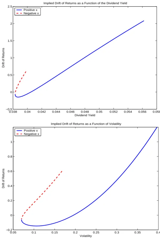
meant to be illustrative, and are consistent with stochastic volatility models estimated by Cher-nov and Ghysels (2002), among others. These parameter values imply that the unconditional standard deviation of volatility is 11%. We set C = 26.1, which matches the average price-dividend ratio in data of 24.5. In Figure 6, we plot points corresponding to a range of plus and minus three unconditional standard deviations ofxfor these parameter values.
The top panel of Figure 6 plots the expected return as a function of the dividend yield implied by the Stein-Stein model. Interestingly, because the Stein-Stein model parameterizes volatility, |x|, rather than variance, there is no one-to-one correspondence between expected returns and dividend yields. We show two branches corresponding to negative and positivex. The negativexbranch produces a much steeper relation between expected returns and dividend yields than the positive x branch. For positive x below the average dividend yield (4.4%), there is a non-monotonic hook-shaped relation between expected returns and dividend yields. However, one failure of the Stein-Stein model is that it cannot account for the variation of dividend yields observed in data. In the top plot of Figure 6, dividend yields range only from approximately 3.8% to 5.6% for a plus and minus three standard bound of xaround its mean, which is substantially smaller than the approximately 1% to 10% range of dividend yields in the data.
In the bottom plot of Figure 6, we graph the implied risk-return trade-off. Again, because the Stein-Stein model assumes an AR(1) process for x, there are multiple risk-return trade-off curves. The risk-return trade-trade-off for negative x is always sharply increasing, whereas the risk-return trade-off for positivexhas a pronounced non-monotonic U-shape pattern for levels of volatility less than 20%. For volatility values higher than 15%, the expected stock return becomes a sharply increasing function of volatility. According to the Stein-Stein model, the risk-return relation will be very hard to pin down empirically because of the non-monotonic relation and multiple correspondence between risk and return. Studies like French, Schwert and Stambaugh (1987) and Bollerslev, Engle and Wooldridge (1988) find only weak support for a positive risk-return trade-off, while Ghysels, Santa-Clara and Valkanov (2005) find a significant and positive relation. On the other hand, Campbell (1987) and Nelson (1991) find significantly negative relations. Glosten, Jagannathan and Runkle (1993) and Scruggs (1998) report that the risk-return trade-off is negative, positive, or close to zero, depending on the specification employed. Brandt and Kang (2004) find a conditional negative, but unconditionally positive, relation between the aggregate market mean and volatility. From Figure 6, it is easy to see that depending on the sample period of low, average, or high volatility, the expected return relation could be flat, upward-sloping, or downward-sloping.
To understand why the risk-return relation in the top panel of Figure 6 generally slopes upwards for large absolute values of x, consider the following intuition. The price-dividend ratiof in the Stein-Stein economy is given byf =C−1exp(−12x2/σ¯x), which is a decreasing