Clothing Simulation and Animation

(1)

SIGGRAPH 2003 COURSE# 29:

“Clothing Simulation and Animation”

Course Notes

Hyeong-Seok Ko

Seoul National University

David Breen

California Institute of Technology

Michael Hauth

University of Tübingen

Ronald Fedkiw

Stanford University

Rob House

Organizers:

Lecturers:

(2)

About the Course

A character appearing with fashionable clothing can add another dimension of richness to 3D

animation. Looking at the degree of detail in these days' character animation, it is easily inferable

that realistic, stable, fast clothing animation technique will be in an ever increasing demand. This

course is targeted to intermediate level animation researchers. It provides an introduction to

state-of-the-art techniques for simulating and animating clothing.

The course begins by an introduction which is organized as a “tutorial within course” so that even

beginners can get a comprehensive idea how cloth simulation is done. It may serve as a summary

of the whole course, and also guide attendees what specific items should be learned in the

subsequent lectures.

The three most fundamental issues for simulating cloth - the physical model, numerical techniques,

and collision handling - are presented during the next 2.5 hours. In the first session, the course

describes low- level models of cloth, its representation by a set of particles and the simulation of its

movement through the evaluation of a set of differential equations. The second session of the course

will describe how to solve the differential equations and how to handle the collisions. Since the

equations tend to be stiff, serious instability problems are possible. Numerical techniques that can

avoid the instabilities will be presented. Collision detection and response are important issues when

simulating clothing. We present methods for detecting cloth/body and cloth/cloth collisions and

incorporating the appropriate response to the collisions into simulation.

In Physical Model of Cloth I (0.75 hour), Dr. Breen will present early work on cloth modeling,

supplemented with a rich collection of still images and animations that spans the last 15 years of

cloth modeling research. In Physical Model of Cloth II (0.5 hour) Prof. Ko will present the later

updates on the interacting particles model of cloth, including the post-buckling instability and

immediate buckling assumption. Numerical Techniques for Cloth Simulation (0.75 hour) will be

lectured by Michael Hauth. Collision Detection/Hand ling will be lectured by Prof. Fedkiw, who is

the author of the paper "Robust Treatment of Collisions, Contact and Friction for Cloth Animation"

in SIGGRAPH 2002.

(3)

feature film Stuart Little. Towards the end, animation researchers will hear vivid voices from

animators: “what needs to be done further?”

Prerequisites

Rudimentary knowledge of computer graphics, computer animation, geometric modeling, linear

algebra, and numerical computing

Course Schedule

Course Title: Clothing Simulation and Animation

Course Number: 29

Component 1: Overview and Modeling

1:45 Introduction – Ko

2:15 Physical Model of Cloth I – Breen

3:00 Physical Model of Cloth II – Ko

3:15 Break

Component 2: Simulation and Animation

3:30 Physical Model of Cloth II (continued) – Ko

3:45 Numerical Techniques for Cloth Simulation – Hauth

4:30 Collision Detection/Handling – Fedkiw

(4)

Course Speakers

Prof. Hyeong -Seok Ko

Director of Graphics & Media Lab

Seoul National University

[email protected]

Hyeong-Seok Ko is an associate professor in the School of Electrical Engineering at Seoul National

University. Currently, he is the Director of Graphics and Media Lab at the same university, and is

actively developing the techniques for realizing Digital Actors, the actors created by computer

graphics technology which are so real that people cannot tell if they are animated or captured from

the real world. Specific areas of current research include cloth animation, hairstyle modeling and

animation, facial animation, physically-based motion retargeting. He has published two

SIGGRAPH papers and numerous journal articles in the above topics. Before joining Seoul National

University, he has held an assistant professor position at the University of Iowa. Ko received B.A.

and M.S. degrees in Computer Science from Seoul National University in 1981 and 1985. He

received a Ph.D. degree in Computer and Information Science from University of Pennsylvania.

He was the conference co-chair of Computer Animation 2001 conference, and the program co-chair

of Computer Animation 2003 conference, which was held at Rutgers University on May 8~9, 2003.

He will serve as the program co-chair of Pacific Graphics 2004, which will be held in Seoul in 2004.

Dr. David E. Breen

Senior Research Scientist

Center for Advanced Computing Research

California Institute of Technology

[email protected]

David Breen is a Senior Research Scientist at the Center for Advanced Computing Research at the

California Institute of Technology. Prior to this, he was the Assistant Director of Caltech's

Computer Graphics Laboratory. He has held research positions at the European Computer-Industry

Research Centre, the Fraunhofer Institute for Computer Graphics, and the Rensselaer Design

Research Center (formerly the RPI Center for Interactive Computer Graphics). His research

interests include level set models for computer graphics, volume segmentation, large data

visualization, and geometric modeling. Breen received a B.A. degree in Physics from Colgate

University in 1982. He received M.S. and Ph.D. degrees in Computer and Systems Engineering

(5)

SIGGRAPH tutorials. Breen is currently the program co-chair of the ACM Symposium on

Computer Animation. He is also the co-editor of the book Cloth Modeling and Animation (AK

Peters).

Michael Hauth

Research Staff

Computer Graphics Laboratory (GRIS)

University of Tübingen

[email protected]

Michael Hauth is a member of the research staff of the Computer Graphics Laboratory (GRIS) at the

University of Tübingen. He studied computer sciences, physics and mathematics at the University

of Tübingen. He received a Diploma (M.Sc.) in computer sciences (1999) and a Diploma (M.Sc.) in

mathematics (2000) from the University of Tübingen. In 2000/2001 he held a visiting post as

research assistant at the Numerical Analysis Group of the University of Geneva.

Prof. Ronald Fedkiw

Computer Science Dept.

Stanford University

[email protected]

Fedkiw received his Ph.D. in Mathematics from UCLA in 1996 and did postdoctoral studies both at

UCLA in Mathematics and at Caltech in Aeronautics before joining the Stanford Computer Scie nce

Department. He was awarded a Packard Foundation Fellowship, a Presidential Early Career Award

for Scientists and Engineers (PECASE), an Office of Naval Research Young Investigator Program

Award (ONR YIP), a Robert N. Noyce Family Faculty Scholarship, two distinguished teaching

awards, etc. Currently he is on the editorial board of the Journal of Scientific Computing and the

IEEE Transactions on Visualization and Computer Graphics, and participates in the reviewing

process of a number of journals and funding agencies. He has published approximately 35 research

papers in computational physics, computer graphics and vision, as well as a new book on level set

methods. For the past two years, he has been a consultant with Industrial Light + Magic.

Robert House

Senior Technical Director

Sony Imageworks, Culver City, California

[email protected]

(6)

Contents

A.

Introduction (Slides)

B.

David Baraff and Andrew Witkin, "Large Steps in Cloth Simulation". (excerpted from the

Proceedings of SIGGRAPH 1998)

C.

Physical Model of Cloth I (Slides)

D.

David Breen, Donald House and Michael Wozny, Predicting the Drape of Woven Cloth

Using Interacting Particles”. (excerpted from the Proceedings of SIGGRAPH 1998)

E.

Cloth/Clothing Modeling and Animation Bibliography, Compiled by David Breen

F.

Physical Model of Cloth II (Slides)

G.

Kwang-Jin Choi and Hyeong-Seok Ko, "Stable but Responsive Cloth". (excerpted from the

Proceedings of ACM SIGGRAPH 2002)

H.

Numerical Techniques for Cloth Simulation (Slides)

I.

Numerical Techniques for Cloth Simulation (written by Hauth)

J.

Bridson, R., Fedkiw, R. and Anderson, J., "Robust Treatment of Collisions, Contact and

Friction for Cloth Animation". (excerpted from the Proceedings of SIGGRAPH 2002)

(7)

Clothing Simulation

and Animation

Organizers:

Hyeong

-

Seok

Ko

David Breen

Lecturers:

Michael

Hauth

Ronald

Fedkiw

Rob House

SIGGRAPH 2003 Course #29:

“

Clothing Simulation and Animation”

Clothing Simulation and Animation

”

Welcome to

SIGGRAPH 2003 Course #29:

(8)

Character animation

Game industry

Fashion industry

Textile industry

The Technique is in High Demand from

The Demand will Continuously Grow.

Realistic cloth

Interactive cloth

Stable cloth

Complex cloth

Collision detection/handling

The Technique is full of Challenges

(9)

Organizers and Lecturers

Hyeong

-

Seok

Ko

Seoul National Univ.

in the order of appearance

…

David Breen

Caltech

Michael

Hauth

Univ. of

Tubingen

Ronald

Fedkiw

Stanford Univ.

Rob House

Sony Pictures

Imageworks

Learn how cloth simulation works

Learn cloth simulation fundamentals

Physical model of cloth

Numerical techniques

Collision detection

Learn clothing animation process in film

industry

Goal of the Course

(10)

1

stst

Session

1.

Introduction (

Ko

, 30min.)

2.

Physical Model of Cloth I (Breen, 45min.)

3.

Physical Model of Cloth II (

Ko

, 30min.)

2

ndnd

Session

1.

Numerical Techniques for Cloth Simulation (

Hauth

, 45min.)

2.

Collision Detection/Handling (

Fedkiw

, 30min.)

3.

Clothing Animation at Sony Pictures

Imageworks

(House,

30min.)

Course Schedule

People who have some experiences on

animation research, and want to initiate

clothing animation

Visual artists who want to understand the

underlying process of clothing animation

Not targeted to world experts of the

subject

Target Audience of the Course

(11)

Introduction

How Cloth Simulation Works?

Hyeong

-

Seok

Ko

Seoul National Univ.

Graphics & Media Lab

Goal of this 30 minutes

Serves as a tutorial within the course

What is the big picture of the whole process?

“

How cloth simulation works?

”

Understands the structure of this course

Guides what specific items should be learned

in the subsequent sessions

(12)

Finding Governing Equation

What is the physical model behind cloth?

)

(

1

F

x

E

M

x

w

How does it Work?

What is the physical model behind cloth?

)

(

1

F

x

E

M

x

w

How does it Work?

David Breen

(13)

Finding Governing Equation

Solving the Equation

Uses numerical techniques

It is not that simple job

How does it Work?

)

(

1

F

x

E

M

x

w

Finding Governing Equation

How does it Work?

“

Numerical Techniques for Cloth Simulation

”

Michael

(14)

Solving the Equation

Collision Detection/Handling

This topic has been studied for a while

But cloth simulation is full of challenging

cases

How does it Work?

“

”

How does it Work?

Ronald

(15)

Finding Governing Equation

Creating Clothed Characters

Constructing garments

Rendering surface details

A lot more

…

How does it Work?

“

Clothing Animation at Sony Pictures

Imageworks

”

How does it Work?

Rob House

(16)

How Cloth Simulation Works?

Let

’

s take a closer look!

How to Represent Cloth?

As a set of particles

(17)

Particle

-

based Cloth Simulation

Repeat the following:

1.

Find the new position of particles

2.

Draw the surface from the particles

History of particle

-

based cloth modeling

“

Physical Model of Cloth I

”

We assume particles move according to some

governing equation.

1

(

E

)

x

M

F

x

w

x

: vector, the geometric state

M

: diagonal matrix, mass distribution of the cloth

E

: a scalar function of x, cloth

’

s internal energy

F

: a function of x and x

’

, other forces acting on cloth

Physically

(18)

Notations

(m

1

, x

1

)

(m

2

, x

2

)

(m

3

, x

3

)

(m

i

, x

i

)

Newton

’

s Equation (ma=F)

(m

1

, x

1

)

(m

2

, x

2

)

(m

i

, x

i

)

¦

forces

i

x

M

»

¼

º

«

¬

ª

i

m

M

0

Bottom

-

up approach

What kind of forces are acting on each particle?

(19)

Forces resulting from Potential Energy

mgy

E

y

F

mg

z

E

y

E

x

E

x

E

w

)

0

,

0

(

)

,

(

&

Example: gravity field

?

Problem of finding forces reduces to

finding the potential energy function.

In Cloth,

Potential energy is related to deformations.

Stretch / Shear / Bending

What are the potential energy functions for

each type of deformation?

E

_stretch_stretch

,

E

_shear_shear

,

E

_bending_bending

(20)

The Potential Function

bending

shear

stretch

E

So, governing

eq

looks like

i i

x

i

x

E

x

E

x

E

x

E

x

M

»

¼

º

«

¬

ª

w

»¼

º

«¬

ª

w

bending

shear

stretch

(21)

There are also other kind of forces

i

x

i

F

x

E

x

M

i

»¼

º

«¬

ª

w

Putting all particles into a vector

…

(m

1

, x

1

)

(m

2

, x

2

)

(m

3

, x

3

)

(m

i

, x

i

)

»

¼

º

«

¬

ª

N

x

1

(22)

i

x

i

F

x

E

x

M

i

»¼

º

«¬

ª

w

F

x

E

x

M

w

)

(

1

F

x

E

M

x

w

Putting all particles into a vector

…

Steps for Finding Governing

Eqs

Determine the potential energy functions

for each type of deformations.

Obtain the total internal force by

summing space

-

derivatives of the

potential functions.

(23)

Now, numerically solve

)

(

1

F

x

E

M

x

w

)

)(

(

)

(

1

F

t

x

E

M

t

x

w

If symbolic

If symbolic deriv

deriv. of E is not available

. of E is not available…

…

)

(

1

F

x

E

M

x

w

)

)(

(

)

(

1

F

t

x

E

M

t

x

w

(24)

If symbolic

If symbolic deriv

deriv. of E is not available

. of E is not available…

…

¿

¾

½

¯

®

'

)

,

(

)

,

(

)

,

(

)

(

1

F

x

t

x

t

x

E

t

x

E

M

t

x

)

(

1

F

x

E

M

x

w

)

)(

(

)

(

1

F

t

x

E

M

t

x

w

Numerical Integration

)

)(

(

)

(

1

F

t

x

E

M

t

x

w

while(1) {

compute the force part at t;

compute

accel

,

vel

, pos;

t = t +

'

t;

}

(25)

Animators love large

'

t.

Large

'

t can cause inaccuracy.

But that

’

s OK if result is visually pleasing.

Large

'

t can cause more serious problem.

Stability issues:

We want both stability and large

'

t.

We want to use large

'

t

Numerical Techniques for Cloth Simulation (

Hauth

)

Why unstable when wrinkles are formed?

A physical instability

Not a numerical instability

Numerical techniques cannot solve the problem

“

Use immediate buckling assumption

”

Improvements in realism, stability, speed

Post

-

buckling Instability

Physical Model of Cloth II (

(26)

Undetected collision can cause a lot of trouble.

Cloth simulation is abundant of challenging

cases for collision detection.

An interesting challenge: simulate garments

formed by multiple layers of cloth.

We have to generate cloth movement due to

collisions.

Collisions in Cloth Simulation

“

”

(

Fedkiw

)

A lot more is needed

Garment construction

Rendering the surface details of cloth

The process used by Sony Pictures

Imageworks

is revealed.

We can hear vivid voices from animators

“

What needs to be done further?

”

How Stuart Little was Clothed?

“

(27)

Finding Governing Equation

Garment Construction

Other Fashioning Features

Real

-

time Simulation

Parts

Covered

and

Not Covered

Particle Model

Continuum Model

Parts

(28)

Large Steps in Cloth Simulation

David Baraff

Andrew Witkin

Robotics Institute

Carnegie Mellon University

Abstract

The bottle-neck in most cloth simulation systems is that time steps must be small to avoid numerical instability. This paper describes a cloth simulation system that can stably take large time steps. The simulation system couples a new technique for enforcing constraints on individual cloth particles with an implicit integration method. The simulator models cloth as a triangular mesh, with internal cloth forces derived using a simple continuum formulation that supports modeling operations such as local anisotropic stretch or compres-sion; a unified treatment of damping forces is included as well. The implicit integration method generates a large, unbanded sparse lin-ear system at each time step which is solved using a modified jugate gradient method that simultaneously enforces particles’ con-straints. The constraints are always maintained exactly, independent of the number of conjugate gradient iterations, which is typically small. The resulting simulation system is significantly faster than previous accounts of cloth simulation systems in the literature.

Keywords—Cloth, simulation, constraints, implicit integration,

physically-based modeling.

1

Introduction

Physically-based cloth animation has been a problem of interest to the graphics community for more than a decade. Early work by Ter-zopoulos et al. [17] and TerTer-zopoulos and Fleischer [15, 16] on de-formable models correctly characterized cloth simulation as a prob-lem in deformable surfaces, and applied techniques from the me-chanical engineering and finite element communities to the prob-lem. Since then, other research groups (notably Carignan et al. [4] and Volino et al. [20, 21]; Breen et al. [3]; and Eberhardt et al. [5]) have taken up the challenge of cloth.

Although specific details vary (underlying representations, nu-merical solution methods, collision detection and constraint meth-ods, etc.), there is a deep commonality amongst all the approaches: physically-based cloth simulation is formulated as a time-varying partial differential equation which, after discretization, is numeri-cally solved as an ordinary differential equation

¨ x=M−1 −∂_∂E_x +F . (1) In this equation the vector x and diagonal matrix M represent the geometric state and mass distribution of the cloth, E—a scalar

func-tion of x—yields the cloth’s internal energy, and F (a funcfunc-tion of x andx) describes other forces (air-drag, contact and constraint forces,˙

internal damping, etc.) acting on the cloth.

In this paper, we describe a cloth simulation system that is much faster than previously reported simulation systems. Our system’s faster performance begins with the choice of an implicit numerical integration method to solve equation (1). The reader should note that the use of implicit integration methods in cloth simulation is far from novel: initial work by Terzopoulos et al. [15, 16, 17] applied such methods to the problem.1 _{Since this time though, research on}

cloth simulation has generally relied on explicit numerical integra-tion (such as Euler’s method or Runge-Kutta methods) to advance the simulation, or, in the case of of energy minimization, analogous methods such as steepest-descent [3, 10].

This is unfortunate. Cloth strongly resists stretching motions while being comparatively permissive in allowing bending or shear-ing motions. This results in a “stiff” underlyshear-ing differential equa-tion of moequa-tion [12]. Explicit methods are ill-suited to solving stiff equations because they require many small steps to stably advance the simulation forward in time.2_{In practice, the computational cost}

of an explicit method greatly limits the realizable resolution of the cloth. For some applications, the required spatial resolution—that is, the dimension n of the state vector x—can be quite low: a reso-lution of only a few hundred particles (or nodal points, depending on your formulation/terminology) can be sufficient when it comes to modeling flags or tablecloths. To animate clothing, which is our main concern, requires much higher spatial resolution to ad-equately represent realistic (or even semi-realistic) wrinkling and folding configurations.

In this paper, we demonstrate that implicit methods for cloth overcome the performance limits inherent in explicit simulation methods. We describe a simulation system that uses a triangular mesh for cloth surfaces, eliminating topological restrictions of rect-angular meshes, and a simple but versatile formulation of the inter-nal cloth energy forces. (Unlike previous metric-tensor-based for-mulations [15, 16, 17, 4] which model some deformation energies as quartic functions of positions, we model deformation energies only as quadratic functions with suitably large scaling. Quadratic energy models mesh well with implicit integration’s numerical properties.) We also introduce a simple, unified treatment of damping forces, a subject which has been largely ignored thus far. A key step in our simulation process is the solution of an O(n)×O(n)sparse lin-ear system, which arises from the implicit integration method. In this respect, our implementation differs greatly from the implemen-tation by Terzopoulos et al. [15, 17], which for large simulations

1_{Additional use of implicit methods in animation and dynamics work}

in-cludes Kass and Miller [8], Terzopoulos and Qin [18], and Tu [19].

(29)

used an “alternating-direction” implicit (ADI) method [12]. An ADI method generates a series of tightly banded (and thus quickly solved) linear systems rather than one large sparse system. (The price, however, is that some of the forces in the system—notably between diagonally-adjacent and non-adjacent nodes involved in self-collisions—are treated explicitly, not implicitly.) The speed (and ease) with which our sparse linear systems can be robustly solved—even for systems involving 25,000 variables or more—has convinced us that there is no benefit to be gained from using an ADI method instead (even if ADI methods could be applied to irregular triangular meshes). Thus, regardless of simulation size, we treat all forces as part of the implicit formulation. Even for extremely stiff systems, numerical stability has not been an issue for our simulator.

1.1

Specific Contributions

Much of the performance of our system stems from the development of an implicit integration formulation that handles contact and ge-ometric constraints in a direct fashion. Specifically, our simulator enforces constraints without introducing additional penalty terms in the energy function E or adding Lagrange-multiplier forces into the force F. (This sort of direct constraint treatment is trivial if equa-tion (1) is integrated using explicit techniques, but is problematic for implicit methods.) Our formulation for directly imposing and maintaining constraints is harmonious with the use of an extremely fast iterative solution algorithm—a modified version of the conju-gate gradient (CG) method—to solve the O(n)×O(n)linear sys-tem generated by the implicit integrator. Iterative methods do not in general solve linear systems exactly—they are run until the solu-tion error drops below some tolerance threshold. A property of our approach, however, is that the constraints are maintained exactly, re-gardless of the number of iterations taken by the linear solver. Addi-tionally, we introduce a simple method, tailored to cloth simulation, for dynamically adapting the size of time steps over the course of a simulation.

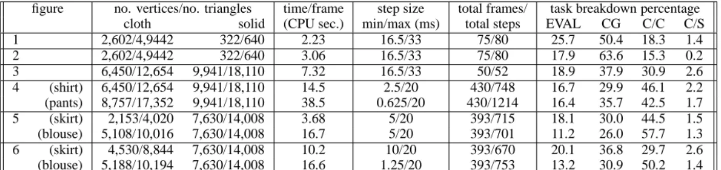
The combination of implicit integration and direct constraint sat-isfaction is very powerful, because this approach almost always al-lows us to take large steps forward. In general, most of our simu-lations require on average from two to three time steps per frame of 30 Hz animation, even for (relatively) fast moving cloth. The large step sizes complement the fact that the CG solver requires rel-atively few iterations to converge. For example, in simulating a 6,000 node system, the solver takes only 50–100 iterations to solve the 18,000×18,000 linear system formed at each step. Addition-ally, the running time of our simulator is remarkably insensitive to the cloth’s material properties (quite the opposite behavior of ex-plicit methods). All of the above advantages translate directly into a fast running time. For example, we demonstrate results similar to those in Breen et al. [3] and Eberhardt et al. [5] (draping of a 2,600 node cloth) with a running time just over 2 seconds per frame on an SGI Octane R10000 195 Mhz processor. Similarly, we show gar-ments (shirts, pants, skirts) exhibiting complex wrinkling and fold-ing behavior on both key-framed and motion-captured characters. Representative running times include a long skirt with 4,530 nodes (8,844 triangles) on a dancing character at a cost of 10 seconds per frame, and a shirt with 6,450 nodes (12,654 triangles) with a cost varying between 8 to 14 seconds per frame, depending on the un-derlying character’s motion.

1.2

Previous Work

Terzopoulos et al. [15, 17] discretized cloth as a rectangular mesh.

ing from the use of implicit integration techniques were solved, for small systems, by direct methods such as Choleski factorization, or using iterative techniques such as Gauss-Seidel relaxation or conju-gate gradients. (For a square system of n nodes, the resulting linear system has bandwidth√n. In this case, banded Choleski

factoriza-tion [6] requires time O(n2₎_{.) As previously discussed, Terzopoulos}

et al. made use of an ADI method for larger cloth simulations.

Following Terzopoulos et al.’s treatment of deformable surfaces, work by Carignan et al. [4] described a cloth simulation system using rectangular discretization and the same formulation as Ter-zopoulos et al. Explicit integration was used. Carignan et al. recog-nized the need for damping functions which do not penalize rigid-body motions of the cloth (as simple viscous damping does) and they added a force which damps cloth stretch and shear (but not bend). Later work by the same group includes Volino et al. [20], which focuses mainly on collision detection/response and uses a tri-angular mesh; no mention is made of damping forces. The system uses the midpoint method (an explicit method) to advance the simu-lation. Thus far, the accumulated work by this group (see Volino et

al. [21] for an overview) gives the only published results we know of

for simulated garments on moving characters. Reported resolutions of the garments are approximately two thousand triangles per gar-ment (roughly 1,000 nodal points) [21] with running times of sev-eral minutes per frame for each garment on an SGI R4400 150 Mhz processor.

Breen et al. [3] depart completely from continuum formulations of the energy function, and describe what they call a “particle-based” approach to the problem. By making use of real-world cloth material properties (the Kawabata measuring system) they produced highly realistic static images of draped rectangular cloth meshes with reported resolutions of up to 51×51 nodes. The focus of this work is on static poses for cloth, as opposed to animation: thus, their simulation process is best described as energy minimization, although methods analogous to explicit methods are used. Speed was of secondary concern in this work. Refinements by Eberhardt

et al. [5]—notably, the use of higher-order explicit integration

meth-ods and Maple-optimized code, as well as a dynamic, not static treat-ment of the problem—obtain similarly realistic results, while drop-ping the computational cost to approximately 20–30 minutes per frame on an SGI R8000 processor. No mention is made of damp-ing terms. Provot [13] focuses on improvdamp-ing the performance of ex-plicit methods by a post-step modification of nodal positions. He it-eratively adjusts nodal positions to eliminate unwanted stretch; the convergence properties of this method are unclear. A more compre-hensive discussion on cloth research can be found in the survey pa-per by Ng and Grimsdale [9].

2

Simulation Overview

In this section, we give a brief overview of our simulator’s architec-ture and introduce some notation. The next section derives the linear system used to step the simulator forward implicitly while section 4 describes the specifics of the internal forces and their derivatives that form the linear system. Section 5 describes how constraints are maintained (once established), with a discussion in section 6 on col-lision detection and constraint initialization. Section 7 describes our adaptive step-size control, and we conclude in section 8 with some simulation results.

(30)

The same component notation applies to forces: a force f∈IR3n

act-ing on the cloth exerts a force fion the ith particle. Real-world cloth

is cut from flat sheets of material and tends to resist deformations away from this initial flat state (creases and pleats not withstanding). We capture the rest state of cloth by assigning each particle an un-changing coordinate(ui, vi)in the plane.3 Section 4 makes use of

these planar coordinates.

Collisions between cloth and solid objects are handled by pre-venting cloth particles from interpenetrating solid objects. Our cur-rent implementation models solid objects as triangularly faced poly-hedra. Each face has an associated thickness and an orientation; par-ticles found to be sufficiently near a face, and on the wrong side, are deemed to have collided with that face, and become subject to a con-tact constraint. (If relative velocities are extremely high, this simple test may miss some collisions. In this case, analytically checking for intersection between previous and current positions can guarantee that no collisions are missed.) For cloth/cloth collisions, we detect both face-vertex collisions between cloth particles and triangles, as well as edge/edge collisions between portions of the cloth. As in the case of solids, close proximity or actual intersection of cloth with it-self initiates contact handling.

2.2

Energy and Forces

The most critical forces in the system are the internal cloth forces which impart much of the cloth’s characteristic behavior. Breen et

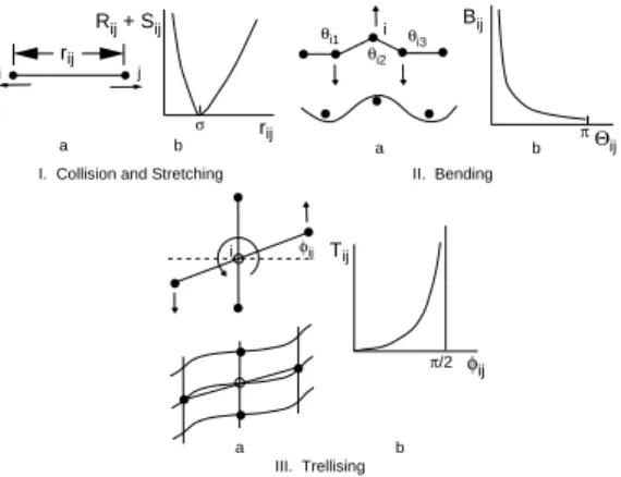
al. [3] describes the use of the Kawabata system of measurement

for realistic determination of the in-plane shearing and out-of-plane bending forces in cloth. We call these two forces the shear and bend forces. We formulate the shear force on a per triangle basis, while the bend force is formulated on a per edge basis—between pairs of adjacent triangles.

The strongest internal force—which we call the stretch force— resists in-plane stretching or compression, and is also formulated per triangle. Under normal conditions, cloth does not stretch apprecia-bly under its own weight. This requires the stretch force to have a high coefficient of stiffness, and in fact, it is the stretch force that is most responsible for the stiffness of equation (1). A common prac-tice in explicitly integrated cloth systems is to improve running time by decreasing the strength of the stretch force; however, this leads to “rubbery” or “bouncy” cloth. Our system uses a very stiff stretch force to combat this problem, without any detrimental effects on the run-time performance. While the shear and bend force stiffness co-efficients depend on the material being simulated, the stretch coef-ficient is essentially the same (large) value for all simulations. (Of course, if stretchy cloth is specifically called for, the stretch coeffi-cient can be made smaller.)

Complementing the above three internal forces are three damp-ing forces. In section 5, we formulate dampdamp-ing forces that subdue any oscillations having to do with, respectively, stretching, shear-ing, and bending motions of the cloth. The damping forces do not dissipate energy due to other modes of motion. Additional forces in-clude air-drag, gravity, and user-generated generated mouse-forces (for interactive simulations). Cloth/cloth contacts generate strong repulsive linear-spring forces between cloth particles.

Combining all forces into a net force vector f, the accelerationx¨i

of the ith particle is simplyx¨i=fi/mi, where miis the ith particle’s

mass. The mass miis determined by summing one third the mass 3_{In general, each particle has a unique}₍_u_{, v)}_{coordinate; however, to}

of all triangles containing the ith particle. (A triangle’s mass is the product of the cloth’s density and the triangle’s fixed area in the uv coordinate system.) Defining the diagonal mass matrix M∈IR3n×3n

by diag(M)=(m1,m1,m1,m2,m2,m2, . . . ,mn,mn,mn), we can

write simply that

¨

x=M−1_f₍_x_,_x_˙_). ₍₂₎

2.3

Sparse Matrices

The use of an implicit integration method, described in the next section, generates large unbanded sparse linear systems. We solve these systems through a modified conjugate gradient (CG) itera-tive method, described in section 5. CG methods exploit sparsity quite easily, since they are based solely on matrix-vector multiplies, and require only rudimentary sparse storage techniques. The spar-sity of the matrix generated by the implicit integrator is best repre-sented in block-fashion: for a system with n particles, we deal with an n×n matrix, whose non-zero entries are represented as dense

3×3 matrices of scalars. The matrix is represented as an array of n rows; each row is a linked list of the non-zero elements of that row, to accommodate possible run-time changes in the sparsity pattern, due to cloth/cloth contact. The (dense) vectors that are multiplied against this matrix are stored simply as n element arrays of three-component vectors. The overall implementation of sparsity is com-pletely straightforward.

2.4

Constraints

An individual particle’s position and velocity can be completely controlled in either one, two, or three dimensions. Particles can thus be attached to a fixed or moving point in space, or constrained to a fixed or moving surface or curve. Constraints are either user-defined (the time period that a constraint is active is user-controlled) or auto-matically generated, in the case of contact constraints between cloth and solids. During cloth/solid contacts, the particle may be attached to the surface, depending on the magnitudes of the frictional forces required; otherwise, the particle is constrained to remain on the sur-face, with sliding allowed. The mechanism for releasing a contact constraint, or switching between sliding or not sliding, is described in section 5.

The constraint techniques we use on individual particles work just as well for collections of particles; thus, we could handle cloth/cloth intersections using the technique described in section 5, but the cost is potentially large. For that reason, we have chosen to deal with cloth/cloth contacts using penalty forces: whenever a par-ticle is near a cloth triangle or is detected to have passed through a cloth triangle, we add a stiff spring with damping to pull the parti-cle back to the correct side of the triangle. The implicit solver easily tolerates these stiff forces.

3

Implicit Integration

Given the known position x(t0)and velocityx˙(t0)of the system at

time t0, our goal is to determine a new position x(t0+h)and

veloc-ityx˙(t0+h)at time t0+h. To compute the new state and

veloc-ity using an implicit technique, we must first transform equation (2) into a first-order differential equation. This is accomplished simply by defining the system’s velocity v as v= ˙x and then writing

(31)

The explicit forward Euler method applied to equation (3) ap-proximates1x and1v as 1x 1v =h v0 M−1f0

where the force f0is defined by f0=f(x0,v0). As previously

dis-cussed, the step size h must be quite small to ensure stability when using this method. The implicit backward Euler method appears similar at first:1x and1v are approximated by

1x 1v =h v0+1v M−1_f₍_x 0+1x,v0+1v) . (4) The difference in the two methods is that the forward method’s step is based solely on conditions at time t0while the backward method’s

step is written in terms of conditions at the terminus of the step itself.4

The forward method requires only an evaluation of the function

f but the backward method requires that we solve for values of1x

and1v that satisfy equation (4). Equation (4) is a nonlinear

equa-tion: rather than solve this equation exactly (which would require iteration) we apply a Taylor series expansion to f and make the first-order approximation f(x0+1x,v0+1v)=f0+ ∂ f ∂x1x+ ∂f ∂v1v.

In this equation, the derivative ∂f/∂x is evaluated for the state

(x0,v0)and similarly for∂f/∂v. Substituting this approximation

into equation (4) yields the linear system 1x 1v =h v0+1v M−1(f0+ ∂ f ∂x1x+ ∂f ∂v1v) ! . (5)

Taking the bottom row of equation (5) and substituting1x= h(v0+1v)yields 1v=hM−1 f0+∂ f ∂xh(v0+1v)+ ∂f ∂v1v .

Letting I denote the identity matrix, and regrouping, we ob-tain I−hM−1∂f ∂v−h 2_M−1∂f ∂x 1v=hM−1 f0+h∂ f ∂xv0 (6)

which we then solve for1v. Given1v, we trivially compute1x= h(v0+1v).

Thus, the backward Euler step consists of evaluating f0, ∂f/∂x

and∂f/∂v; forming the system in equation (6); solving the system

for1v; and then updating x and v. We use the sparse data structures

described in section 2.3 to store the linear system. The sparsity pat-tern of equation (6) is described in the next section, while solution techniques are deferred to section 5.

4_{The method is called “backward” Euler because starting from the output}

state(x0+1x,v0+1v)and using a forward Euler step to run the system

backward in time (i.e. taking the step−h(v(t0+h),f(x(t0+h),v(t0+h)))

brings you back to(x0,v0). What is the value in this? Forward Euler takes

4

Forces

Cloth’s material behavior is customarily described in terms of a scalar potential energy function E(x); the force f arising from this energy is f = −∂E/∂x. Equation (6) requires both the vector f

and the matrix∂f/∂x. Expressing the energy E as a single

mono-lithic function—encompassing all aspects of the cloth’s internal behavior—and then taking derivatives is impractical, from a book-keeping point of view. A better approach is decompose E into a sum of sparse energy functions; that is, to write E(x)=P_αE_α(x)where each E_αdepends on as few elements of x—as few particles—as pos-sible.

However, even decomposing E into sparse energy functions is not enough. Energy functions are an undesirable starting point be-cause sensible damping functions cannot be derived from energy functions. Instead, we define internal behavior by formulating a vector condition C(x)which we want to be zero, and then defining the associated energy ask

2C(x)

T_C₍_x₎_{where k is a stiffness constant.}

In section 4.5, we show how sensible damping functions can be con-structed based on this formulation. An added bonus is that starting from this vector-based energy description tends to result in a sim-pler, more compact, and more easily coded formulation for∂f/∂x

than proceeding from an energy function in which the structure of

C has been lost.

4.1

Forces and Force Derivatives

Given a condition C(x)which we want to be zero, we associate an energy function ECwith C by writing EC(x)=k2C(x)

T_C₍_x₎_where

k is a stiffness constant of our choice. Assuming that C depends

on only a few particle, C gives rise to a sparse force vector f. Re-call from section 2.1 that we view the vector f in block form; each element fiis a vector in IR3. For each particle i that C depends

on, fi= −∂ EC ∂xi = − k∂C(x) ∂xi C(x); (7) all the other elements of f are zero.

Similarly, the derivative of f is also sparse. Defining the deriva-tive matrix K=∂f/∂x, the nonzero entries of K are Kijfor all pairs

of particles i and j that C depends on. Again, we treat K in block fashion: K∈IR3n×3n_{, so an element K} ijis a 3×3 matrix. From equation (7), we have Kij= ∂ fi ∂xj = − k ∂C(x) ∂xi ∂C(x) ∂xj T +∂_∂2C(x) xi∂xj C(x) . (8) Additionally, since Kij is a second derivative—that is, Kij =

∂fi/∂xj=∂2E/∂xi∂xj—we have Kij=KTjiso K is symmetric. Note

that since C does not depend on v, the matrix∂f/∂v is zero.

We can now easily describe the internal forces acting on the cloth, by just writing condition functions. Forces and their derivatives are easily derived using equations (7) and (8).

4.2

Stretch Forces

Recall that every cloth particle has a changing position xiin world

space, and a fixed plane coordinate(ui, vi). Even though our cloth is

modeled as a discrete set of points, grouped into triangles, it will be convenient to pretend momentarily that we have a single continuous function w(u, v)that maps from plane coordinates to world space. Stretch can be measured at any point in the cloth surface by

(32)

examin-vdirection is measured bykwvk. (Some previous continuum for-mulations have modeled stretch energy along an axis as essentially

(wT

uwu−1)2, which is a quartic function of position [15, 16, 17, 4].

We find this to be needlessly stiff; worse, near the rest state, the force gradient—a quadratic function of position—is quite small, which partially negates the advantage implicit integration has in exploit-ing knowledge of the force gradient. A quadratic model for energy is, numerically, a better choice.)

We apply this stretch/compression measure to a triangle as fol-lows. Let us consider a triangle whose vertices are particles i, j and

k. Define1x1=xj−xiand1x2=xk−xi. Also, let1u1=uj−ui,

while1u2=uk−uiand similarly for1v1and1v2. We

approxi-mate w(u, v)as a linear function over each triangle; this is equiva-lent to saying that wuand wvare constant over each triangle. This lets us write1x1=wu1u1+wv1v1and1x2=wu1u2+wv1v2.

Solving for wuand wvyields

(wu wv)=(1x1 1x2) 1u1 1u2 1v1 1v2 −1 . (9) Note that x1and x2vary during the simulation but the matrix in the

above equation does not.

We can treat wuand wvas functions of x, realizing that they de-pend only on xi, xjand xkand using equation (9) to obtain

deriva-tives. The condition we use for the stretch energy is

C(x)=a kwu(x)k −bu kw_v(x)k −b_v (10)

where a is the triangle’s area in uvcoordinates. Usually, we set

bu=bv=1, though we need not always do so. In particular, if we want to slightly lengthen a garment (for example, a sleeve) in the u direction, we can increase bu, which causes wuto seek a larger value,

and tends to induce wrinkles across the u direction. Likewise, we might decrease b_vnear the end of a sleeve, inducing a tight cuff, as on a sweatshirt. We have found the ability to control shrink/stretch anisotropically to be an indispensable modeling tool.

4.3

Shear and Bend Forces

Cloth likewise resists shearing in the plane. We can measure the ex-tent to which cloth has sheared in a triangle by considering the inner product wT

uwv. In its rest state, this product is zero. Since the stretch

term prevents the magnitudes of wuand wvfrom changing overly

much, we need not normalize. By the small angle approximation, the product wT

uwvis a reasonable approximation to the shear angle.

The condition for shearing is simply

C(x)=awu(x)Twv(x) with a the triangle’s area in the uvplane.

We measure bend between pairs of adjacent triangles. The con-dition we write for the bend energy depends upon the four particles defining the two adjoining triangles. If we let n1and n2denote the

unit normals of the two triangles and let e be a unit vector parallel to the common edge, the angleθbetween the two faces is defined by the relations sinθ=(n1×n2)

·

e and cosθ=n1

·

n2. We define a

condition for bending by writing simply C(x)=θwhich results in a force that counters bending.5_{The assumption that the stretch}

en-ergy will keep the cloth from stretching much allows us to treat n1, 5_{For reasonably equilateral triangles, as edge lengths decrease, the}

cur-n2and e as having a constant length at each step of the simulation.

This makes differentiatingθwith respect to x a manageable task. Rectangular meshes make it simple to treat bending anisotropi-cally. The uvcoordinates associated with particles make this possi-ble for triangular meshes as well. Given material for which bending in the u andvdirections are weighted by stiffnesses kuand kv, we can emulate this anisotropy as follows. Let the edge between the triangles be between particles i and j, and define1u=ui−ujand

1v=vi−vj. The stiffness weighting for this edge should simply

be

ku(1u)2+kv(1v)2

(1u)2+(1v)2 .

4.4

Additional Forces

To the above forces we also add easily implemented forces such as gravity and air-drag (which is formulated on a per-triangle basis, and opposes velocities along the triangle’s normal direction). When the simulation is fast enough to interact with, we add user-controlled “mouse” forces. These forces and their gradients are easily derived.

4.5

Damping

The energies we have just described are functions of position only. Robust dynamic cloth simulation, however, is critically dependent on well-chosen damping forces that are a function of both position

and velocity. For example, the strong stretch force must be

ac-companied by a suitably strong damping force if we are to prevent anomalous in-plane oscillations from arising between connected particles. However, this strong damping force must confine itself solely to damping in-plane stretching/compressing motions: stretch damping should not arise due to motions that are not causing stretch or compression. Terzopoulos et al.’s [16, 17] treatment of cloth used a simple viscous damping function which dissipated kinetic energy, independent of the type of motion. Carignan et al. [4] im-proved upon this somewhat, borrowing a formulation due to Platt and Barr [11]; however, their damping function—a linear function of velocity—does not match the quartic energy functions of their continuum formulation. In this section we describe a general treat-ment for damping that is independent of the specific energy function being damped.

It is tempting to formulate a damping function for an energy func-tion E(x)by measuring the velocity of the energy, E˙ = _dtdE(x). This is an easy trap to fall into, but it gives nonsensical results. At an equilibrium point of E, the gradient∂E/∂x vanishes. Since

˙

E=(∂E/∂x)T_{x, we find that}_˙ _{E is zero when E is at its minimum,}˙

regardless of the system’s velocityx˙=v. In general,E is always˙

too small near the system’s rest state. Clearly, basing the damping force onE is not what we want to do.˙

We believe that the damping function should be defined not in terms of the energy E, but in terms of the condition C(x)we have been using to define energies. The force f arising from the energy acts only in the direction ∂C(x)/∂x, and so should the damping

force. Additionally, the damping force should depend on the com-ponent of the system’s velocity in the∂C(x)/∂x direction; in other

words, the damping strength should depend on (∂C(x)/∂x)T_x_˙ ₌

˙

C(x). Putting this together, we propose that the damping force d associated with a condition C have the form

(33)

Given the condition functions C we have defined in this sec-tion for stretch, bend and shear forces, we can now add accompa-nying damping forces by applying equation (11). As before, diis

nonzero only for those particles that C depends on, and∂d/∂x has

the same sparsity pattern as∂f/∂x. Differentiating equation (11), we

obtain ∂di ∂xj= − kd ∂ C(x) ∂xi ∂C˙(x) ∂xj T +∂_∂2C(x) xi∂xj ˙ C(x) ! . (12) Note that∂d/∂x is not a second derivative of some function as was

the case in equation (8) so we cannot expect∂d/∂x to be

symmetri-cal. In equation (12), it is the term(∂C(x)/∂xi)(∂C˙(x)/∂xj)Twhich

breaks the symmetry. Anticipating section 5.2, we find it expedi-ent simply to leave this term out, thereby restoring symmetry. This simplification is clearly not physically justifiable, but we have not observed any ill effects from this omission. (Omitting all of equa-tion (12), however, causes serious problems.)

Finally, equation (6) requires the derivative∂d/∂v. SinceC˙(x)=

(∂C(x)/∂x)T_{v, we have} ∂C˙(x) ∂v = ∂ ∂v _∂ C(x) ∂x T v =∂C(x) ∂x .

Using this fact, we can write

∂di ∂vj = − kd∂ C(x) ∂xi ∂C˙(x) ∂vj T = −kd∂ C(x) ∂xi ∂C(x) ∂xj T .

In this case, the result is symmetrical without dropping any terms.

5

Constraints

In this section, we describe how constraints are imposed on indi-vidual cloth particles. The constraints we discuss in this section are either automatically determined by the user (such as geometric at-tachment constraints on a particle) or are contact constraints (gener-ated by the system) between a solid object and a particle. The tech-niques we describe in this section could be used for multi-particle constraints; however, constraints that share particle would need to be merged. Thus, a set of four-particle constraints (such as ver-tex/triangle or edge/edge contacts in the cloth) might merge to form a single constraint on arbitrarily many particles, which would be ex-pensive to maintain. Because of this, we handle cloth/cloth contacts with strong springs (easily dealt with, given the simulator’s underly-ing implicit integration base) and “position alteration,” a technique described in section 6.

At any given step of the simulation, a cloth particle is either com-pletely unconstrained (though subject to forces), or the particle may be constrained in either one, two or three dimensions. Given the differential nature of our formulation, it is the particle’s accelera-tion, or equiva