Testing Financing Constraints on Firm Investment using Variable
Capital
∗
Andrea Caggese
Pompeu Fabra University
First version: February 2003
This version: August 2006
Abstract
We consider a dynamic multifactor model of investment with financing imperfections,
adjustment costs and fixed and variable capital. We use the model to derive a test of
financing constraints based on a reduced form variable capital equation. Simulation results show that this test correctly identifiesfinancially constrainedfirms even when the estimation of firms’ investment opportunities is very noisy. In addition, the test is well specified in
the presence of both concave and convex adjustment costs of fixed capital. We confirm
empirically the validity of this test on a sample of small Italian manufacturing companies. JEL classification: D21, G31
Keywords: Financing Constraints, Investment
∗I am most grateful to Nobu Kiyotaki for his encouragement and valuable feedback on my research. I would
like also to thank Orazio Attanasio, Steven Bond, Martin Browning, Vicente Cunat, Christian Haefke, Francois Ortalo-Magne, Steve Pischke and the anonymous Referee for their valuable comments and suggestions on earlier˙
versions of this paper, as well as the participants at the 2005 ASSA meetings in Philadelphia, the 2003 ESEM Congress in Stockholm, the 2003 CEPR Conference on Entrepreneurship, Financial Markets and Innovation, and at seminars at UPF, LSE, Banco de Espa˜na, University of Copenhagen and Ente Einaudi. All errors are, of course, my own responsibility. Research support from the Financial Markets Group and from Mediocredito Centrale are gratefully acknowledged. Please address all correspondence to: andrea.caggese@upf.edu or Pompeu Fabra University, Department of Economics, Room 1E58, Calle Ramon Trias Fargas 25-27, 08005, Barcelona, Spain
I
Introduction
In order to explain the aggregate behavior of investment and production, it is necessary to understand the factors that affect investment atfirm level. Financing imperfections may prevent firms from accessing externalfinance and make them unable to invest unless internal finance is available. It is therefore important to study the extent to which financing constraints matter forfirms’ investment decisions. This line of inquiry is also relevant for other areas of research, such as the literature on the role of internal capital markets and banks, as well as the macro literature on thefinancial accelerator.
Starting with Fazzari, Hubbard and Petersen (1988), several studies investigate the presence offinancing constraints by estimating the Qmodel of investment with cash flow included as an
explanatory variable.1 They argue informally that under certain conditions, and in the absence of financing frictions, Tobin’s average Q is equal to marginal q,and is a sufficient statistic for
firm investment (Hayashi, 1982). It follows that, conditional onQ,cashflow should affect only
the investment offinancially constrained firms.
The motivation for this paper is that recent studies, starting with Kaplan and Zingales (1997 and 2000), have shown that the correlation betweenfixed investment and cashflow is not a good indicator of the intensity offirmfinancing constraints. In particular Erickson and Whited (2000) and Bondet al (2004) show that errors in measuring the expected profitability of firms explain most of the observed positive correlation between fixed investment and cash flow. Moreover, Gomes (2001), Pratap (2003) and Moyen (2004) simulate industries with heterogeneous firms who may face financing frictions. They show that the correlation between fixed investment and cashflow may be positive for financially unconstrainedfirms, and even larger than that of financially constrainedfirms.2 Finally, Caballero and Leahy (1996) show that the failure of the investment - cashflow correlation as a measure offinancing constraints may be caused not only by the measurement error in Q,but also by misspecification and omitted variable problems.
The objective of this paper is to develop a new financing constraints test that is robust to 1See Hubbard (1998) for a review of this literature.
2
Alti (2003) and Abel and Eberly (2003) and (2004) develop theoretical frameworks in which positive investment-cashflow correlations arise in the absence offinancial markets imperfections.
these problems and has the following properties: i) it is able to detect both the presence and the intensity offinancing constraints onfirm investment; ii) it is efficient even in the presence of large errors in the measurement of the productivity shock; iii) it is well specified under a wide range of assumptions concerning the adjustment costs offixed capital.
The test is derived from a structural model of a risk-neutralfirm that generates output using two complementary factors of production,fixed and variable capital. Fixed capital is irreversible, while variable capital can be adjusted without frictions. Because of an enforceability problem, thefirm can obtain externalfinancing only if it secures it with collateral. The assets of thefirm can only be partially collateralizable and some down payment is needed tofinance investment.
We describe the optimality conditions of the model and we demonstrate that under the hypothesis of financing imperfections, the correlation between financial wealth and variable capital investment is a reliable indicator of the presence of financing constraints. We use this result to develop a formalfinancing constraint test based on a reduced form variable investment equation. This new test has two main advantages with respect to the previous literature. First, variable investment is less influenced by adjustment costs thanfixed investment. This property reduces misspecification and omitted variable problems in the investment equation, thereby making it easier to distinguish the contribution of financial factors from the contribution of productivity shocks tofirms’ investment decisions. Second, whilefixed investment decisions are forward looking, variable investment decisions are mostly affected by the current productivity shock, which is relatively easy to estimate even if only balance sheet data are available. Therefore ourfinancing constraints test does not require the estimation of Tobin’sQ,and it can be applied
also to small privately ownedfirms not quoted on the stock markets. This property of the test is important. The previous investment literature has mainly studied the financing constraints of large firms quoted on the stock markets, even tough financing frictions are mostly relevant for the financing of small privately owned firms.3 One reason for this bias is that the previous
3
Among the exceptions, Himmelberg and Petersen (1994) and Whited (2006) consider data sets of publicly ownedfirms focusing explicitly on small and very smallfirms. Jaramillo, Schiantarelli, and Weiss (1996), Gelos and Werner (2002) and L´izal and Svejnar (2002) study samples of small privately owned firms in developing countries. However the claim that smallfirms do not matter for developed economies, because largefirms account for most of the aggregate employment and output, is not correct. For example, in 1995, smallfirms with less than 100 employees accounted for 37.9% of the total employment in the US economy (source: US Census).
literature focuses mostly on theQmodel, where averageQis computed as the ratio of the market
value of the firm / the replacement value of its assets. However, because the market value is easily measurable only for publicly traded firms, this approach precludes the analysis of the effects offinancing constraints on privately owned firms.4
We study the properties of the new financing constraints test by solving the model and simulating several industries with heterogenousfirms. We show that the sensitivity of variable capital to financial wealth is able to detect both the presence and the intensity of financing constraints on firm investment. This result is robust to both concave and convex adjustment costs offixed capital. More importantly, large observational errors in measuring the productivity shock do not affect the power of the test, because thefinancial wealth of the simulatedfirms has a very low correlation with the current productivity shock.
We verify the validity of this test on two datasets of Italian manufacturing firms. These datasets are very useful for the purpose of this paper for two reasons: i) almost all of thefirms considered are small and not quoted on the stock market; ii) all the firms are also covered by in-depth surveys with qualitative information about the financing problems the firms faced in funding investment.
We estimate the variable investment equation on these datasets and we confirm the pre-dictions of the model. First, the estimated coefficients do not reject the restrictions imposed by the structural model. Second, the sensitivity of variable investment to internal finance is significantly positive forfirms that are likely to face capital markets imperfections (according to the qualitative survey) while it is always very small and not significantly different from zero for the other firms.
This paper contributes to both the theoretical and empirical literature on financing con-straints andfirm investment. The simulation results of this paper are related to Gomes (2001), Pratap (2003) and Moyen (2004). Because we consider both convex and non-convex adjustment
4
One can in principle use other methods to calculate marginalq using only balance sheet data. For example Gilchrist and Himmelberg (1998) apply the VAR approach of Abel and Blanchard (1986) to a panel offirms. But probably the resulting estimate of marginalq is even more noisy than the average Q calculated using the stock market valuation offirms. Therefore thefinancing constraints test based on this measure of marginalq is probably even less reliable than the test based on averageQ.
costs, we are able to clarify the relationship between adjustment costs and the investment-internalfinance relationship. In our benchmark model, fixed capital is irreversible andq is not
a sufficient statistic for investment. In this case, the cashflow - investment sensitivity is highest for financially unconstrained firms, even in the absence of measurement errors in q, as is also
found by Moyen (2004). In the alternative modelfixed capital is subject to convex adjustment costs and q is a sufficient statistic for investment. We show that in this case, the cash flow
- investment sensitivity is a reliable indicator of financing constraints, even in the presence of large measurement errors inq.
Because of its emphasis on the importance of adjustment costs to understand the investment decisions made by firms, this paper is related to Barnett and Sakellaris (1998) and to Abel and Eberly (2002), who analyze the implications of different types of adjustment costs on the relationship between marginalQand investment at thefirm and at the aggregate level. Moreover
it is related to Whited (2006) who shows that, in the presence of fixed costs of investment, constrainedfirms are less likely to undertake a new, large investment project than unconstrained firms, after controlling for expected productivity and for the time elapsed since the last large investment project.
The empirical section of this paper uses a structural model of firm investment to derive a financing constraints test that is based on a simple reduced form linear investment equation. A similar approach is followed by Hennessy, Levy and Whited (2006), who derive an enhanced version of the Q model that allows for the presence of financing frictions and debt overhang.
Carpenter and Petersen (2003) estimate a version of the Q model with cash-flow where the
dependent variable is the growth of total assets of the firm rather than the fixed investment rate.
Our method to test for financing constraints on firm investment can be applied using any reversible factor of production. This paper considers the usage of variable inputs as the depen-dent variable of the test. Therefore it is also related to Kashyap, Lamont and Stein (1994) and Carpenter, Fazzari and Petersen (1998). These authors show that inventories atfirm level are very sensitive to internalfinance, especially for thosefirms a priori more likely to be financially
constrained. With respect to these authors, our paper, in addition to proposing a more rigorous financing constraints test that identifies both the presence and the intensity of financing con-straints, has two further advantages. First, while theflow of the usage of materials is very close to a frictionless variable input, changes in total inventories are potentially subject to adjustment costs of various nature, such as the presence of fixed costs that imply (S,s) type of inventory policies. Therefore the reduced form linear inventory models estimated by Kashyap, Lamont and Stein (1994) and Carpenter, Fazzari and Petersen (1998) are potentially subject to misspecifica-tion problems, which make it difficult to distinguish whether internalfinance significantly affects inventories because of financing frictions or because it is capturing other omitted information. Second, even iffinancing constraints affect inventory decisions, this does not necessarily imply that they also affect the investment in production inputs and the level of production of thefirm. Indeed the very fact that afinancially constrainedfirm can absorb a reduction in cashflow with a reduction in inventories means that it may be able to maintain the desired flow of variable inputs into the production process. Instead, the objective of this paper is precisely to estimate the intensity offinancing constraints on the investment in variable inputs and on the production of the firm.
This paper is organized as follows: section II describes the model. Section III defines the new financing constraints test. Section IV illustrates the simulation results. Section V verifies the validity of the newfinancing constraints test using a balanced panel of Italianfirms and finally, section VI summarizes the conclusions.
II
The model
The aim of this section is to develop a structural model of investment withfinancing constraints and with adjustment costs offixed capital. We consider a risk-neutral firm whose objective is to maximize the discounted sum of future expected dividends. The discount factor is equal to 1/R, whereR= 1 +r,and r is the lending/borrowing risk-free interest rate.
The firm operates with two inputs, kt and lt, fixed and variable capital respectively. The
form:
yt=θtkαtl
β
t withα+β <1. (1)
All prices are constant and normalized to 1. This simplifying assumption will be relaxed in the empirical section of the paper. θt is a productivity shock that follows a stationary
AR(1) stochastic process. For simplicity we assume that variable capital is nondurable and fully depreciates after one period, whilefixed capital is durable:
0<δ <1, (2)
in whichδ is the depreciation rate of fixed capital. Moreover variable capital investment is not subject to adjustment costs, whilefixed capital investment is irreversible:
it+1≥0, (3)
in which it+1 is gross fixed investment:
it+1≡kt+1−(1−δ)kt (4)
We assume full irreversibility for convenience, but the results of the paper would also hold for other types of non-convex adjustment costs, such as partial irreversibility or fixed costs. Moreover in section IV we relax this assumption allowing also for convex adjustment costs.
Financial imperfections are introduced by assuming that new share issues and risky debt are not available. At timetthefirm can borrow from (and lend to) the banks one period debt, with
face valuebt+1, at the market riskless interest rate r.A positive (negative) bt+1 indicates that
thefirm is a net borrower (lender). Banks only lend secured debt, and the only collateral they accept is physical capital. Therefore at time tthe borrowing capacity of the firm is limited by
the following constraints:
bt+1≤υkt+1 (5)
0<υ≤1−δ
dtare dividends. υ is the share offixed capital that can be used as collateral. One possible
justification for constraint (5) is that the firm can hide the revenues from production. Being unable to observe such revenues, the banks can only claim the residual value of thefirm’s physical assets as repayment of the debt (Hart and Moore, 1998).5 If υ = 1−δ then all the residual value of fixed capital is accepted as collateral. This is possible because we assume that the irreversibility constraint (3) does not apply when the firm as a whole is liquidated and all its assets are sold.6
The timing of the model is as follows: new capital purchased in period t−1 generates output in period t. At the beginning of period t the firm’s technology becomes useless with
an exogenous probability 1−γ. In this case the assets of the firm are sold and the revenues are distributed as dividends. Instead with probabilityγ the firm continues activity. Then θt is
realized,ytis produced using kt andlt,the production inputs purchased in the previous period,
and bt is repaid. The exogenous exit probability is necessary in order to generate simulated
industries in which a fraction of firms are financially constrained in equilibrium. If γ = 1 and firms live forever then they eventually accumulate enough wealth to become unconstrained, and the simulated industry always converges to a stationary distribution offinancially unconstrained firms, no matter how tight the financing constraint (5) is.
It is useful to define the net worth of the firmwt, after the debtbt is repaid, as follows:
wt=wtF + (1−δ)kt (7)
WherewF
t isfinancial wealth:
wtF =yt−bt (8)
5
Some authors argue that variable capital has a higher collateral value thanfixed capital (Berger et al, 1996). Nevertheless the results derived in this section are consistent with alternative specifications that allow for a positive collateral value of variable capital.
6
In theory, the interactions betweenfinancing constraints and adjustment costs offixed capital may imply that in some cases thefirm is forced to liquidate the activity to repay the debt, even if it would be profitable to continue. In order to simplify the analysis, we focus in this paper on the set of parameters that do not allow this outcome to happen in equilibrium.
After producing, the firm allocates wFt plus the new borrowing between dividends, fixed capital investment and variable capital investment, according to the following budget constraint:
dt+lt+1+it+1=wtF +bt+1/R (9)
For convenience, we define atas the stock of financial savings:
at≡ −bt
We define a∗ as the minimum level of financial savings such that the borrowing constraint
(5) is never binding for every period j ≥t. The concavity of the production function (1) and the stationarity of the productivity shock θ ensure that a∗ is positive and finite. Intuitively, when at ≥ a∗ the returns from savings are always higher than the maximum losses from the
production activity: ra∗t >max
kt,θt
(lt+1+it−yt). Because the discount factor of thefirm is equal
to 1/R,when at< a∗ thefirm faces future expected financing constraints and always prefers to
retain rather than to distribute earnings. Instead when at ≥a∗ the firm is indifferent between
retaining and distributing net profits. Therefore we make the following assumption:
Assumption 1:if at ≥a∗ then the firm distributes net profits as dividends:
dt=yt−lt+1−it+1+rat ifat ≥a∗t (10)
Equation (10) implies that the firm distributes as dividends the extra savings above a∗.
As-sumption 1 is only necessary to provide a natural upper bound to the value ofwtF,and it does not affect the real investment decisions of thefirm.
Let’s denote the value at time tof the firm, after θt is realized, by Vt(wt,θt, kt):
Vt(wt,θt, kt) = M AX πt
kt+1,lt+1,bt+1 + γ
REt[Vt+1(wt+1,θt+1, kt+1)] (11)
πt=γdt+ (1−γ)wt (12)
Thefirm maximizes (11) subject to equations (5),(6) and (9). Appendix 1 provides a proof
that the optimal policy functions kt+1(wt,θt, kt), lt+1(wt,θt, kt) and bt+1(wt,θt, kt) exist and
In order to describe the optimality conditions of the model, we use equation (9) to substitute
dt in the value function (11). Letµt,λtand φt be the Lagrangian multipliers associated
respec-tively with the irreversibility constraint (3), the borrowing constraint (5) and the non-negativity constraint on dividends (6). The solution of the problem is defined by the following conditions:
φt=Rλt+γEt ¡ φt+1¢ (13) Et µ ∂yt+1 ∂kt+1 ¶ =nRh1 +Et ³ Ψkt+1´i−(1−δ)o−Rµt+ΦtEt ¡ µt+1¢ (14) Et µ ∂yt+1 ∂lt+1 ¶ =Rh1 +Et ³ Ψlt+1´i (15) ³ 1−τk R ´ kt+1+lt+1≤wtF + (1−δ)kt−dt (16) Where: Φt = γ(1−δk) 1 +γEt ¡ φt+1¢ (17) Et ³ Ψkt+1´ = (R−τk)λt−Rγcov ³ φt+1,∂yt+1 ∂kt+1 ´ 1 +γEt ¡ φt+1¢ (18) Et ³ Ψlt+1´ = Rλt− Rγcov ³ φt+1,∂yt+1 ∂lt+1 ´ 1 +γEt ¡ φt+1¢ (19)
Equations (13), (14) and (15) are thefirst order conditions ofbt+1, lt+1 andkt+1 respectively.
Equation (16) combines the budget constraint (9) and the collateral constraint (5) and implies that the down payment necessary to buy kt+1 and lt+1 must be lower than the residual net
worth after paying the dividends. By iterating forward equation (13) we obtain:
φt=R
∞
X
j=0
Et(λt+j) (20)
Equation (20) implies that as long as there are some current or future expected financing constraints, then φt > 0 and the firm does not distribute dividends: dt = 0. Equation (14)
represents the optimality condition for thefixed capitalkt+1.The left-hand side is the marginal
©
R£1 +Et
¡
Ψkt+1¢¤−(1−δ)ªis the shadow cost of buying one additional unit offixed capital net of its residual value (1−δ).The termEt
¡
Ψkt+1¢is equal to zero if thefirm is notfinancially constrained today or in the future.The termµtmeasures the shadow cost of a currently binding irreversibility constraint. Futureexpected irreversibility constraints Et
¡
µt+1¢are multiplied by the termΦt,which is an increasing function of the expected shadow value of money 1+E
¡ φt+1¢. Therefore the more the firm expects to be financially constrained in the future, the higher the cost of future expected irreversibility constraints. Equation (15) is the optimality condition for the variable capital lt+1. The term Et
¡ Ψl
t+1
¢
is directly related to λt, the Lagrange multiplier
of the borrowing constraint (5).
If constraint (16) is not binding thenλt= 0. In this case equations (14) and (15) determine
the optimal unconstrained capital levels ktu+1 and lut+1. If kut+1 is greater than (1−δ)kt, then
the irreversibility constraint (3) is not binding, the Lagrange multiplier µt is equal to zero and ©
kt∗+1, lt∗+1ª, the optimal investment choices, are determined by©ktu+1, lut+1ª. Ifkut+1 is smaller than (1−δ)kt then the irreversibility constraint is binding. kt+1 is constrained to be equal to
(1−δ)kt, and equations (14) and (15) can be solved to determine ltic+1 and µict . In this case
the optimal investment choices©k∗t+1, l∗t+1ªare determined by ©(1−δ)kt, lict+1
ª
.The collateral
constraint is instead binding whenfinancial wealth is not sufficient as a down payment forkt∗+1
and lt∗+1,even ifdt= 0: ³ 1−τk R ´ kt∗+1+l∗t+1 > wt+ (1−δ)kt (21)
In this case the constrained levels of capital ktc+1 and lct+1 are such that: ³
1−τk
R
´
ktc+1+lct+1 =wt+ (1−δ)kt (22)
and the solution is determined by the values ktc+1, lct+1 , λt and µt that satisfy equations (3),
(14), (15) and (22).
III
A new test of
fi
nancing constraints based on variable capital
One important property of variable capital is that equation (15) is not directly affected by the irreversibility constraint of fixed capital. Thefinancing constraints test developed in this paper
uses this property plus the fact that the termEt
¡
Ψlt+1¢,which summarizes the effect offinancing constraints on variable capital investment, is a monotonously decreasing and convex function of
wi,tF,as stated in the following proposition:
Proposition 1 We define wtmax(θt, kt) as the level of financial wealth such that the firm does
not expect to befinancially constrained now or in the future. It follows, for a given value of the
state variables θt and kt and for wFt < wtmax, that Et
¡
Ψlt+1¢ is positive and is decreasing and
convex in the amount of internal finance:
∂Et ¡ Ψlt+1¢ ∂wFt <0 , ∂2Et ¡ Ψlt+1¢ ∂¡wFt ¢2 >0 and wF lim t→wtM AX Et ³ Ψlt+1 ´ = 0
Conversely if wFt ≥wtmax thenEt¡Ψlt+1
¢ = 0
Proof: see appendix 2.
Proposition 1 applied to equation (15) establishes a link between financing imperfections and the real investment decisions of firms. It says that when a firm is financially constrained then the availability of internalfinance increases the investment in variable capital and reduces its marginal return. It is important to note that proposition 1 cannot be applied to fixed capital investment because of the presence of the irreversibility constraint. If the irreversibility constraint is binding, then kt+1 = (1−δ)kt and µt >0.In this case a change in the intensity
offinancing constraints, that causes a change inEt
¡ Ψk
t+1
¢
in equation (14), affects the value of
µtbut does not affectfixed capital investment.
Therefore we propose a newfinancing constraints test that applies proposition 1 to variable capital investment decisions. If we take logs of both sides of equation (15) and we solve for lnlt+1 we obtain: lnlt+1 = 1 1−β ln β R+ 1 1−β lnEt(θt+1) + α 1−βlnkt+1− 1 1−βln h 1 +Et ³ Ψlt+1´i (23)
Proposition 1 allows us to substitute 1 +Et
¡
Ψlt+1¢with a negative and convex function of wtmax
wF t . We approximate it as follows: 1 +Et ³ Ψlt+1´= (wmaxt /wFt )η (24)
in which η is an indicator of the intensity of the financing constraints. The more the firm is financially constrained (in the model, this corresponds to a lower value of υ, which tightens the financing constraints), the more the investment of the firm is sensitive to internal finance (meaning that Et
¡
Ψlt+1¢ increases more rapidly as wtF decreases) and the larger η is. wtmax is not observable in reality, but it is itself a function of the other state variables. Intuitivelywtmax
increases inEt(θi,t+1) because a higher productivity increases the financing needs of thefirm,
and conditional onEt(θi,t+1) it decreases in kt,because a higher existing stock offixed capital
implies that more financial wealth can be used to finance variable capital. Sincekt+1 is highly
correlated withkt,our simulations show that a good approximation of wmaxt is the following:
wmaxt =wmax[Et(θt+1)]ζkωt+1 (25)
Using equations (24) and (25) in (23), and lagging equation (23) by one period, we obtain the following reduced form variable capital equation:
lnlt=π0+π1lnEt−1(θt) +π2lnkt+π3lnwtF−1+εt (26) π0≡ 1 1−β ln µ β Rw max ¶ ; π1≡ 1−ηζ 1−β ; π2 ≡ α−ηω 1−β ; π3 ≡ η 1−β (27) The termεt includes the approximation errors. When estimating equation (26) with the
empir-ical data it may also include measurement errors as well as unobservable productivity shocks. Such problems are dealt with in the estimations in the empirical section of the paper.
The new financing constraints test is based on the coefficientπ3.In the absence offinancing
frictions η is equal to zero. This implies that π3 = 0, π1 = 1−1β and π2 = 1−αβ. Therefore π1
and π2 can be used to recover the structural elasticities αand β. In the presence of financing
constraints η and π3 are instead positive. The intuition is the following: suppose a financially
unconstrained firm receives a positive productivity shock at time t−1, so that lnEt−1(θt) is
high. Thisfirm increaseslt up to the point that the marginal return on variable capital is equal
to its user cost. Alternatively a financially constrained firm can only invest in variable capital if it hasfinancial wealth available. For this firm lnlt is less sensitive to the productivity shock
lnEt−1(θt) and is positively affected by the amount offinancial wealth lnwtF−1.It is important to
capital, and it implies that variable investment may be significantly financially constrained even after a negative shock, when θt−1 and Et−1(θt) are low. The negative shock implies that
kt−1 is relatively high, and the firm would prefer to reduce it, but kt is constrained to be
not smaller than (1−δ)kt−1. In this situation a financially unconstrained firm would choose a
relatively high level oflt,because the two factors of productions are complementary. In contrast
a financially constrainedfirm is forced to cut variable capital when it has not enough financial wealth available, and therefore the lower lnwtF−1 is, the lower lnltis.
This financing constraints test has the following useful properties: i) it does not require the estimation of marginalq,but only of the productivity shockθ.Unlikeq,θis not a forward looking variable. Therefore any error in measuring the profitability of thefirm probably implies a smaller measurement error inθthan in q. Moreoverθ can be estimated from balance sheet data, and it can be easily applied to datasets of small privately ownedfirms not quoted on the stock market. ii) Although it is based on a simple reduced form investment equation, this test allows the recovery of the structural parameters αandβ.The estimates of αand β provide an additional robustness check of the validity of the model. iii) Simulation results presented in the next section show that equation (26) is also able to detect the intensity of financing constraints whenfixed capital is subject to convex adjustment costs rather than to the irreversibility constraint. The intuition is that in both cases equation (26) is well specified, because the information concerning the adjustment costs offixed capital is summarized by kt.
A
Alternative testing strategy
As an alternative to equation (26), one could transform equation (15) as follows:
βyt lt =R h 1 +Et−1 ³ Ψlt ´i +εyt (28) whereεyt ≡βEt−1(yt)−yt
lt is an expectational error. By taking logs and rearranging, we obtain
the following:
loglt= logβ+ logyt−log
n R h 1 +Et−1 ³ Ψlt ´i +εyt o (29)
Therefore εyt enters nonlinearly in equation (29). If εyt is small relative to Et−1 ¡ Ψlt¢, one can approximate log©R£1 +Et−1 ¡ Ψlt¢¤+εytª with log©R£1 +Et−1 ¡
Ψlt¢¤ª+εyt, and obtain the following:
lnlt=π0+π1lnyt+π2lnwFt−1+ε
y
t (30)
In theory, equation (30) could be used for the purpose of estimating the intensity offinancing constraints. However our simulations of the calibrated model indicate thatεyt is likely to be large because its volatility is driven by the volatility of the idiosyncratic productivity shock. They also show that the nonlinearity of εyt in equation (29) may considerably reduce the precision of the financing constraints test based on equation (30), especially when the number of observations in the sample is small. Therefore in the empirical section of this paper we focus on the estimation of equation (26).
IV
Simulation results
In this section we use the solution of the model to simulate the activity of many firms. These
are ex ante identical and are subject to an idiosyncratic productivity shock that is
uncorre-lated across firms and autocorrelated for each firm. We simulate several industries in order to verify whether equation (26) is able to detect the intensity of financing constraints on firms investment. We adopt the same methodology commonly used in empirical applications since the seminal paper of Fazzari, Hubbard and Petersen (1988). We use a priori information to select a subsample of firms more likely to face financing imperfections, and then we compare the sensitivity of investment to internalfinance for this group with respect to the other firms. All simulations assume that prices and interest rate are constant. As our objective is to analyze the effects of financing constraints at firm level, the partial equilibrium nature of this exercise does not restrict the analysis in any important way. In one set of simulated industries, firms becomefinancially constrained when the borrowing constraint (5) is binding, and their internal finance is not sufficient tofinance all profitable investment opportunities. In another set of in-dustries,firms are notfinancially constrained becauseυis so high that the borrowing constraint (5) is never binding with equality. We also make a further distinction. In one set of industries
fixed capital is irreversible and in another, fixed capital is subject to the following quadratic adjustment costs function:
µ(it) =b 1 2 ∙ it kt−1 ¸2 kt−1 (31)
In the context of our model, equation (31) determines the following reduced form investment equation: it kt−1 =−1 b + 1 b qt−1 1 +φt−1 +Φt−1 (32) Φt−1 ≡ υ b λt−1 1 +φt−1; qt−1 ≡Et−1 ∙ dVt(wt,θt, kt) dkt ¸
In the absence offinancing frictions bothΦt−1 andφt−1 are equal to zero, and equation (32)
simplifies to a linear relationship between marginalq and the investment rate:
it kt−1 =−1 b + 1 bqt−1 (33)
The idiosyncratic shock is modeled as follows (in the remainder of the paper we include the subscriptito indicate thei−thfirm):
yt=θIi,t ³ θi,tkαtl β t ´ withα+β<1 (34)
θi,t is a persistent shock and θIi,t is an i.i.d. shock:
lnθi,t=ρlnθi,t−1+εi,t (35)
0<ρ<1; εi,t ∼iid ¡ 0,σ2ε¢ for all i (36) lnθIi,t =εIi,t (37) εIi,t∼iid¡0,σ2εI ¢ for all i (38)
The persistent shockθis necessary to match the volatility and the persistence infirm invest-ment. The i.i.d. shockθI matches the volatility of profits and ensures that they are negative for a significant share offirms in the simulated industry. Both shocks are important because they
allow the simulatedfirms to have realistic dynamics of both investment andfinancial wealth. If we only allow for the persistent shockθ(by settingσ2εI = 0),not only is the volatility of profits
of simulatedfirms too low, but these also never have negative profits, which instead are observed for a large share of firm-year observations in the sample used for the empirical analysis in the next section.
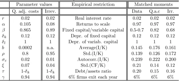
The dynamic investment problem is solved using a numerical method (see appendix 3 for details). The model is parameterized assuming that the time period is one year. Table I summarizes the choice of parameters. The risk-free real interest rate r is equal to 2%, which
is the average real return on a 1-year US T bill between 1986 and 2005. The sum of αand β matches returns to scale equal to 0.97. This value is consistent with studies on disaggregated data that find returns to scale to be just below 1 (Burnside, 1996). Moreover, because in the model there are nofixed costs of production, even such a small deviation from constant returns is sufficient to generate, for the set of benchmark parameters, average profits in the simulated firms that are relatively large and consistent with the empirical evidence. β is set to match the ratio of fixed capital over variable capital. In the model, variable capital fully depreciates in one period, and therefore we consider as variable capital the sum of materials cost and wages, and we consider asfixed capital land, buildings, plant and equipment. Using yearly data about manufacturing plants from the NBER-CES database (which includes information about the cost of materials), we calculate afixed capital/variable capital ratio between 0.5 and 0.7 for the 1980-1996 period. The other parameters are the following: the depreciation rate offixed capitalδis set equal to 0.12;b,ρandσεmatch the average, standard deviation, and autocorrelation of thefixed
investment rate of the US Compustat database, as reported in Gomes (2001);σ2εI matches the
standard deviation of the cashflow/fixed capital ratio;υis set to match the average debt/assets ratio of US corporations; γ is equal to 0.94,implying that in each period a firm exits with 6% probability. This value is consistent with the empirical evidence aboutfirms’ turnover in the US (source: Statistics of U.S. Businesses, US Census Bureau). The second part of table I reports the matched moments. The simulated industries do not match perfectly the empirical moments, given the presence of nonlinearities in the mapping from the parameters to the moments, but
they are sufficiently close for our purpose.
We simulate 50000firm-year observations, which can be interpreted as an industry where we observe every firm in every period of activity, and where a firm that terminates its activity is replaced by a newbornfirm. The initial wealth of a newbornfirm is equal to 40% of the average fixed and variable capital of a financially unconstrained firm. This initial endowment ensures that financing constraints are binding for a non-negligible fraction of firms in the simulated industries. The initial fixed capital of a newborn firm is ex ante optimal, conditional on its initial wealth and the expectation as regards the initial productivity shock.Tables II-V report
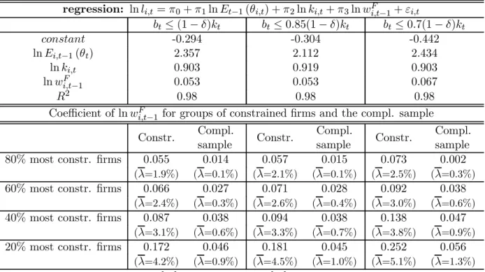
the estimation results from the simulated data. In these tables we do not report the standard deviations of the estimated coefficients, because all coefficients are strongly significant. Table II reports the estimation results of equation (26). It shows that the new test is always able to identify morefinancially constrained firms because the coefficient of lnwF is positive in the
industries with financing frictions and is otherwise equal to zero. In the bottom part of table II we compare the groups of most constrained firms and the complementary samples (the test statistic of the difference in the coefficients across groups is not reported because it is always significantly different from zero). We sortfirms into groups of morefinancially constrainedfirms using the average value of the Lagrangian multiplierλi,t:
λi= Ti
X
i=1
λi,t (39)
whereTi is the number of years of operation offirmi. In the industries withfinancing frictions,
the financing constraint is not always binding. This is because firms accumulate wealth, and become progressively less likely to face a bindingfinancing constraint. Therefore the higher λi
is, the higher the intensity offinancing problems forfirmi.
The middle part of table II shows that the coefficient of lnwF also identifies the intensity of financing constraints because its magnitude increases with the magnitude ofλi in each industry.
Intuitively, the higher the value ofλi,the morefirmihas observations with a bindingfinancing
constraint and the more variable capital is sensitive tofinancial wealth.
of variable capital tofinancial wealth, is on average larger in the industry with the irreversibility constraint than in the industry with convex adjustment costs. λ is higher in the former case because the irreversibility offixed capital significantly increases the impact offinancing frictions on variable capital investment. This happens not only because variable capital is the only factor of production that absorbs wealth fluctuations when the irreversibility constraint is binding, but also because when both constraints are binding a firm has too much fixed capital and not enough funds to invest in variable capital. The unbalanced use of the two factors of production reduces revenues andfinancial wealth and it increases the intensity offinancing constraints. On the contrary, in the industry with quadratic adjustment costs,fixed investment is allowed to be negative and afirm can absorb a negative productivity shock by reducing bothfixed and variable capital. The other estimated coefficients are consistent with the predictions of the model. In the industry withoutfinancing frictions, the estimated coefficientsπ1 and π2 are equal to 1−1β and
α
1−β. In the industries with financing frictions, π1 and π2 are also nonlinear functions of the
parametersζ and ω.
The approximations in equations (24) and (25) imply that equation (26) is correctly spec-ified also in the presence of financing frictions. Therefore it is important to verify that these approximations are correct, and that they do not bias the estimated coefficient of lnwF. First, we verify that the approximation (24) is confirmed by the data. We show this by regressing log£1 +Et
¡
Ψlt+1¢¤ on log(wmaxt /wFt ).The estimation yields η = 0.024,with a very high good-ness of fit (R2 = 0.977). This relationship is also shown graphically in figure 1. Second, we
take the logs of equation (25) and we estimate it with OLS. The R2 of the regression is 0.91,
suggesting that the effect of the omitted variable lnwmaxt in equation (26) should be absorbed by lnEt−1(θt) and lnkt,and should not bias significantly the coefficient of lnwtF−1. We verify
this claim by estimating a version of equation (26) where lnwmaxt−1 is explicitly included as a regressor. The bottom part of table II reports the estimation results, which are very similar to those illustrated above, and confirm that the coefficient of lnwFt−1 is a reliable indicator of the intensity offinancing constraints.
are perfectly observable. However in reality the productivity shockθtis estimated using balance
sheet data. Therefore table III reports the estimation results of equation (26) where lnEt−1(θt)
is observed with noise:
lnEt−1(θt)∗ = lnEt−1(θt) +κt−1
κt−1 is an i.i.d. error drawn from a normal distribution with mean 0 and varianceσ2κ.The first
column of table III replicates the results in the first column of table II. The second and third columns include a measurement error in lnEt−1(θt), with a “noise-to-signal” ratio (the ratio
of σ2κ to the variance of lnEt−1(θt)) equal to 0.25 and 1 respectively. The next three columns
repeat the same analysis for the economy with the irreversibility constraint. The results show that measurement errors cause a negative bias in the coefficient of lnwtF−1.But because the bias is small, this coefficient is still a reliable indicator of the intensity of financing constraints. It is positive only for financially constrainedfirms, and a higher value of this coefficient for a group of firms always signals that this group is more financially constrained than the complementary sample. The only exception is in the third column: in this case when the measurement error is very large and firms are not very constrained (in the economy with quadratic adjustment costs λ is much smaller than 1% for all firms except the 20% most constrained ones), then the coefficient of lnwtF−1 becomes negative, even though it is still increasing in the intensity of financing constraints.
The measurement error in the productivity shock has little effect on the coefficient of lnwtF,
because these two variables are nearly uncorrelated in the industries withfinancing constraints (see table II). This happens despite lagged cash flow, which is one of the determinants of financial wealth, being positively correlated to the productivity shock. There are two reasons for the low correlation between lnEt−1(θt) and lnwFt−1: i)firms that facefinancing imperfections
accumulatefinancial wealth. This means thatwFt−1increases as the accumulated savings increase, and it becomes less sensitive to currentfluctuations in cashflow; ii) equation (7) shows that the net worth of the firm is the sum of financial wealth wFt and the residual value of fixed capital (1−δ)kt. Because the productivity shock is persistent, when θt−1 and Et−1(θt) are low, it is
also likely that θt−2 was low, so that the firm did not invest in fixed capital in the past, and
a larger fraction of its wealth wt−1 was invested in financial wealthwFt−1. The same reasoning
applies whenEt−1(θt) is high. This “composition effect” implies a negative correlation between
financial wealth and the productivity shock, and it counterbalances the positive correlation effect induced by the cashflow.
We have so far assumed that the residual value of capital is entirely collateralisable.In other
words, there is no discount in the liquidation value of the firm’s fixed assets. This assumption increases the leverage of the simulatedfirms and gets it closer to the empirical value. However, in reality, distressedfirms often sell capital atfire-sale prices. Therefore in table IV we estimate equation (26) for industries with different values ofυ. Thefirst column replicates the results of table II, withυ= 1−δ. The second and third columns considerυ= 0.85(1−δ) andυ= 0.7(1−δ) respectively. They show that the lower the collateral value of capital, the higher the intensity offinancing constraints and the coefficient of lnwFt−1.
Summing up, the simulation results illustrated in tables II-IV suggest that the coefficient of lnwF in equation (26) is a precise and reliable indicator of financing constraints, even in the presence of different types of adjustment costs of fixed capital and large observational errors in the productivity shock.
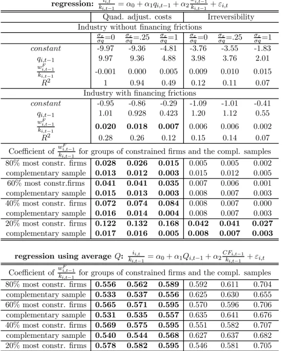
In the remainder of this section we compare the performance of this new test with a test based on theq model offixed capital:
ii,t ki,t−1 =α0+α1qi,t−1+α2 wi,tF−1 ki,t−1 +εi,t (40)
Table V shows the estimation results of equation (40). In the σε
σq=.25 and
σε
σq=1 columns
there is a measurement error inq, with a noise-to-signal ratio equal to 0.25 and 1 respectively.
In thefirst half of table V, adjustment costs are quadratic. In the absence offinancing frictions, the investment ratio ii,t
ki,t−1 is determined by equation (33) and therefore qi,t−1 is a sufficient statistic for ii,t
ki,t−1.As a consequence, the coefficient of
wF i,t−1
ki,t−1 is equal to zero.In the presence of financing frictions the coefficient of w
F i,t−1
ki,t−1 is positive, significant, and increasing in the intensity offinancing constraints, even in the presence of measurement errors, because ii,t
by equation (32), and w
F i,t−1
ki,t−1 is negatively correlated with the omitted term 1 +φt−1.Therefore the first half of table V shows that when adjustment costs are convex, equation (40) does a good job of identifying financing constraints, even in the presence of measurement errors in q.
On the contrary, in the second part of table V we consider the industry with irreversibility of fixed capital. Hereq is no longer a sufficient statistic for investment, and the coefficient of w
F i,t−1
ki,t−1 is positive for unconstrainedfirms because financial wealth conveys relevant information about investment. Moreover the coefficient of w
F i,t−1
ki,t−1 is small for financially constrained firms because for them, most of thefluctuations in wealth are absorbed by variable capital. As a consequence, fixed capital investment is more sensitive to financial wealth for less constrained than for more constrained firms for almost all of the sorting criteria. Thus equation (40) is not useful for identifyingfinancing constraints, as is also found in Gomes (2001), Pratap (2003), Moyen (2004) and Hennessy and Whited (2006).
A more direct comparison with the previous literature is provided at the bottom of table V, where we use averageQto replace the unobservable marginal q, and we use the cashflow ratio
CFi,t−1
ki,t−1 as the explanatory variable that captures financing frictions. The results show that the cash flow coefficient is highly significant both in the constrained and unconstrained industries, as also found by Moyen (2004). However such coefficient is not a good indicator of the presence offinancing constraints in the presence of fixed capital irreversibility.
V
Empirical evidence
In this section we verify empirically the validity of the new test offinancing constraints described in the previous section on a sample of small and medium Italian manufacturing firms. The sample is obtained by merging the two following datasets provided by Mediocredito Centrale: i) a balanced panel of more than 5000firms with company accounts data for the 1982-1991 period.7
This is a subset of the broader dataset of the Company Accounts Data Service, which is the most reliable source of information on the balance sheet and income statements of Italianfirms,
7
The original sample had balance sheet data from 1982 to 1994, but we discarded the last three years of balance sheet data (1992, 1993 and 1994) from the sample, because of discrepancies and discontinuities in some of the balance sheet items, probably due to changes in accounting rules in Italy in 1992.
and it has often been used in empirical studies onfirm investment (e.g. Guiso and Parigi, 1999). ii) The four Mediocredito Centrale Surveys on small and medium Italian manufacturing firms. The surveys were conducted in 1992, 1995, 1998 and 2001. Each Survey covers the activity of a sample of more than 4400 small and medium manufacturing firms in the three previous years. The samples are selected balancing the criterion of randomness with that of continuity. Each survey contain three consecutive years of data. After the third year, 2/3 of the sample is replaced and the new sample is then kept for the three following years.
The information provided in the surveys includes detailed qualitative information on prop-erty structure, employment, R&D and innovation, internationalization and financial structure. Among thefinancial information, each Survey asks specific questions aboutfinancing constraints. In addition to this qualitative information, Mediocredito Centrale also provides, for most of the firms in the sample, an unbalanced panel with some balance sheet data items going back as far as 1989. Examples of published papers that use the Mediocredito Centrale surveys are Basile, Giunta and Nugent (2003) and Piga (2002).
The main dataset used in this section is obtained by merging thefirms in the balanced panel of the Centrale dei Bilanci with thefirms in the 1992 Mediocredito Survey. The merged sample is composed of 812firms, for which we have a unique combination of very detailed balance sheet data and detailed qualitative information about financing constraints. As a robustness check in section VI,E we consider an alternative dataset based on the 1998 and 2001 surveys. This dataset is larger but has less detailed balance sheet data and less precise information about financing constraints.
Regarding the main dataset, we eliminatefirms without the detailed information concerning the composition of fixed assets (that do not distinguish between plant and equipment on the one side and land and building on the other side), ending up with 561 firms. We further eliminatefirms that merged orfirms that split during the sample period. The remaining sample is composed of 415firms, virtually none of which is quoted on the stock markets. The information onfinancing constraints is contained in the investment section of the 1992 Survey. This section requests detailed information regarding the most recent investment projects aimed at improving
thefirm’s production capacity. Thefirm indicates both the size of the project and the years in which such project was undertaken. 95% of all the answers concern projects undertaken between 1988 and 1991. Among thefinancial information, thefirm is asked whether it had difficulties in financing such project because of:
a) “lack of medium-long term financing”; b) “high cost of banking debt”; c) “lack of guar-antees”.
It is worthwhile to notice that the selection of the firms in this sample is biased towards less financially constrained firms, for at least two reasons: i) the balanced panel only includes firms that have been continually in operation between 1982 and 1992, thus excluding newfirms and firms that ceased to exist during the same period because of financial difficulties; ii) by eliminating mergers we eliminatefirms in profitable businesses that merged with other companies because of theirfinancing problems.
For the empirical specification of the financing constraints test we consider the following production function:
yi,t=θi,tki,tα−1l β
i,tn
γ
i,t (41)
All variables are in real terms, and are the following: yi,t = total revenues (during period
t, firm i); ki,t−1 = replacement value of plant, equipment and intangible fixed capital (end of
periodt−1,firmi);li,t = cost of the usage of materials (during periodt,firmi);ni,t = labor cost
(during periodt,firmi). Detailed information about all the variables is reported in appendix 4.
With respect to equation (1) in the theoretical model, equation (41) includes labor as a factor of production and it includes fixed capital as lagged by one period. Therefore we assume that fixed capital installed in period t will become productive from period t+ 1 on. Under these
assumptions the first order condition for variable capital is still represented by equation (15). By using equation (41) in (15) we get:
βEt(θt+1)kαtl β−1 t+1n γ t+1 =R h 1 +Et ³ Ψlt+1´i (42)
Equation (42) implies that proposition 1 still holds, conditional also onnt.Moreover we can
capital equation:
lnli,t=π0+ai+dt+π1lnθi,t−1+π2lnki,t−1+π3lnni,t+π4lnwFi,t−1+εi,t, (43)
in whichεi,tis the error term, and lnθi,t−1 is the productivity shock, which is derived by taking
the expectation of equation (35) and by noting that lnEt−1(θi,t) =ρ+σ
2 ε
2 + lnθi,t−1.The term
ρ+ σ2ε
2 is included in the constant term. The coefficient π4 measures the intensity of financing
constraints. Under the assumption of no financing constraints the reduced form coefficients π1,π2 and π3 can be used to recover the structural parametersα,β and γ:
π1 = 1 1−β;π2 = α 1−β;π3 = γ 1−β (44)
In the model the user cost of variable capital is constant and equal to R for financially
un-constrained firms. In reality the user cost of capital may vary across firms and over time for
several reasons unrelated tofinancing imperfections, such as transaction costs, taxes, and risk. Therefore in equation (43) we also include firm and year dummy variables, respectivelyai and
dt.These capture, among other things, the changes in the user cost of capital acrossfirms and
over time for all thefirms.
We estimate the productivity shock lnθi,t−1 from the Solow residual of the production
func-tion at the beginning of period t. The method used is robust to the presence of decreasing
returns to scale and to heterogeneity in technology (see appendix 6 for details).
We compute wFt ,the netfinancial wealth at the beginning of period t,by using the budget constraint (9) at timet−1 to substitutebt in (8):
wFt =Πt+Rt ¡ wFt−1−dt−1 ¢ (45) Πt≡yt−Rt(lt+it−1)
In the model,Πtare profits generated from the investment in period t−1, and are realized at
the beginning of periodt. Therefore we estimateΠt as the operative profits during periodt−1
(value of production minus the cost of production inputs). Moreover we estimate¡wFt−1−dt−1
¢ as the net short-termfinancial assets (after dividend payments) plus the stock offinished goods inventories at the beginning of periodt−1. We include the stock of finished goods inventories
because most of such goods will be transformed into cashflow during period t−1. Rt is equal
to one plus the average real interest rate during periodt−1.
The concave transformation of wealth in equation (24) can be computed only ifwFt is positive. The simulations of the model show that, for reasonable parameter values, financial wealth is always positive in an economy with financing frictions. This is because such frictions at the same time reduce the maximum amount of borrowing and give incentive tofirms to accumulate financial assets. The empirical data are consistent with thisfinding, because the variablewFt is positive for 95.2% firm-year observations. Among the 4.8% negative observations, nearly half are excluded as outliers. In order to include the remaining negative observations, we consider an alternative definition offinancial wealth based on the following modification of the borrowing constraint (9):
bi,t+1≤υki,t+1+bi, (46)
in whichbi represents the collateral value offirmiin addition to the residual value of its assets.
It can be interpreted as intangible collateral assets (for example from relationship lending). In this case it is appropriate to modify (24) as follows:
1 +Et
³
Ψlt+1´ = (wmaxt /wtF)η ifwFt ≤wmax (47)
wFt = wtF +bi (48)
We estimate bi as the average borrowing of a firm in excess of the collateral value of the
firm’s fixed assets. The valuebi is found to be positive for 125 firms (30% of the total). wFt is
positive for 97.5%firm-year observations.
The estimation of equation (43) is complicated by the endogeneity of the regressors. First, all the regressors are most likely correlated to thefirm-specific effectai.Second, lnni,tis endogenous
because it is simultaneously determined with lnli,t. Third, the other right-hand side variables
are predetermined, but they may still be endogenous and correlated to εi,t. In other words,
if all the relevant information about future expected productivity is summarized by lnθi,t−1,
then εi,t should be uncorrelated to the predetermined regressors. Otherwise an unobservable
εi,t and cause an error-regressor correlation. The same problem may be caused by a persistent
measurement error. In this case, a suitable estimation strategy is tofirst difference equation (43) in order to eliminate the unobservablefirm-specific effectai, and then estimate it with a GMM
estimation technique, using the available lagged levels and first differences of the explanatory variables as instruments. In this case, the set of instruments is different for each year and equation (43) is estimated as a system of cross sectional equations, each one corresponding to a different periodt(Arellano and Bond, 1991). More recent lags are likely to be better instruments,
but they may be correlated with the error term if the unobservable productivity shock is very persistent. The test of overidentifying restrictions can be used to assess the orthogonality of the instruments with the error term. Moreover, under the assumption thatE(∆zi,t−j, ai) = 0,
withz=nlnθi,t,lnki,t,lnwFi,t,lnni,t
o
,∆zi,t−j is a valid instrument for equation (43) estimated
in levels. Blundell and Bond (1998) propose a System GMM estimation technique that uses both the equation in level (instrumented using laggedfirst differences), and the equation infirst differences (instrumented using lagged levels). They show, with Monte Carlo simulations, that the System GMM estimator is much more efficient than the simple GMM estimator when the regressors are highly persistent, and when the number of observations is small. These properties are particularly useful in our context. Table XV shows the test of the validity of the instruments for the estimation of equation (43). The upper part reports the p-value of theHansen Jstatistic
that tests the orthogonality of the instruments. The bottom part of table XV reports the F statistic of the excluded instruments and the partial R2 from Shea (1997). The table shows
that the t-1 to t-3first differences as instruments for the equation in levels and the t-3 levels as instruments for the equation in first differences are not rejected by the orthogonality test and are sufficiently correlated to the regressors for the coefficients of equation (43) to be identified.
The primary objective of this empirical analysis is to verify that the coefficient of lnwi,tF−1in equation (43) is a precise indicator of the intensity offinancing constraints. We do it by using the qualitative information provided by the Mediocredito Survey, which allows us to selectfirms more likely to be financially constrained. We also selectfirms according to some exogenous criteria commonly used in the previous literature as indicators of financing imperfections: i) dividend
policy:firms that have higher cost (or rationing) of externalfinance than of internally generated finance are less likely to distribute dividends. Therefore the observed dividend policy should be correlated to the intensity of financing constraints. ii) Size and age: smaller and youngerfirms usually are more subject to informational asymmetries that may generatefinancing constraints. More specifically, we estimate equation (43) for subsamples of firms selected according to the dummy variable Dxi,t, which is equal to 1 if the firm i belongs to the specific group x, and zero otherwise. Among the direct criteria, Dhs identifies firms that declare too high a cost of banking debt (13.7% of allfirms);Dlc identifies firms with lack of medium-long term financing
(13.2% of allfirms).8 Among the indirect criteriaDage identifiesfirms founded after 1979 (16% of allfirms);Ddivpolidentifiesfirms with zero dividends in any period (33.4% of allfirms);Dsize
identifiesfirms with less than 65 employees (in 1992) (16% of all firms).
We estimate the coefficients of equation (43) separately for each group of firms and for the complementary sample by interacting the above criteria with the explanatory variables, the constant, the yearly dummies and all the instruments. The Dhs and Dlc dummies are potentially endogenous, because an unobservable shock may at the same time be correlated with the likelihood of declaringfinancing constraints and with the error term in equation (43). However, this problem is not likely to bias the GMM estimates of equation (43) because we exclusively adopt cross sectional selection rules. In other words, Heckman (1979) shows that the selection bias can be represented as an omitted variable problem. But we do not allowfirms to wander in and out of the constrained group, and therefore the omitted term is also constant over time for eachfirm and is absorbed by thefixed effect in the estimation. Because the GMM estimator used in the paper is based onfirst differences, it is robust to this type of cross sectional bias.
Another potential problem is measurement errors in the Survey. For example, at the time of the 1992 Survey, Mediocredito Centrale was a state-controlledfinancial institution whose main 8We do not selectfirms according to the question concerning “lack of guarantees” because only 2% of firms
answer positively, and almost all of those are already included in theDlcandDhsgroups.
Also, among all thefirms in the sample 8% did not declare any investment project in the Mediocredito Survey, and therefore did not answer the questions aboutfinancing constraints. We keep thesefirms in the unconstrained sample, but one may also argue that perhaps some of thesefirms did not invest precisely because they may have beenfinancially constrained. In order to control for this possibility we repeated the analysis excluding suchfirms from the sample, obtaining results very similar to those reported in the following sections.
objective was to provide subsidized credit to small and mediumfirms. Therefore it may be that thosefirms declaring the problem of “lack of medium-long termfinancing” were actually sending strategic messages to the institution. However virtually all of the subsidized credit administrated by Mediocredito Centrale has been directed to the South of Italy. Indeed, among the firms in the 1992 Mediocredito Survey none of thefirms from the North and Central Italy had benefited from any subsidized credit, while as much as 58.7% of thefirms from the South had. Therefore this problem can be controlled for by excluding from theDlcgroup the firms from South Italy, which are 5% of the total (dummyDlc
−south).
Another problem is that the Dlc = 1 group may include some distressed firms that need more banking debt in order to survive, not because they need to finance a profitable project. The structure of the 1992 Survey, which only allowsfirms to declare financing problems if they actually undertook a new investment project, should avoid this problem. Nonetheless, we control for this by considering an alternative selection criterion that excludes from the Dlc group also the 10% offirms with lower average ratio of gross profits over sales (dummy D−lcs.&lowyeld).
Table VI illustrates the summary statistics. The whole sample is composed almost entirely of small firms. 50% of the firms have under 123 employees and 90% under 433. Virtually all of these firms are privately owned and not quoted on the stock market. Likely financially constrained firms do not show significant differences with respect to the other firms in terms of size, growth rate of sales, investment rates, riskiness (volatility of output) and gross income margin. The most noticeable differences concern the financial structure. Firms that declare financing constraints are less wealthy, on average pay higher interest rates on banking debt and have a lower net income margin.
Table VII shows the estimation results of equation (43) for the whole sample and for the groups selected according to the “direct criteria” dummies. In thefirst column we use the data from the 1986-91 period, for which we have available the full set of instruments. In the other columns we estimate the model for the shorter 1988-91 period.9
The full sample estimates in thefirst two columns show that the coefficients of lnθi,t,lnki,t−1
9
We restrict the sample because the Mediocredito Survey refers to the 1989-91 period, but 5% of the investment projects surveyed actually started in 1988.
and lnni,t are all significant and all have the expected sign and size. The coefficient of lnwFi,t is
very small in magnitude and not significantly different from zero. This suggests that financing constraints do not affect a large share offirms in the sample, and is consistent with the informa-tion from the Mediocredito Survey, where only 22% of thefirms state some problem infinancing investment.
The remaining columns in table VII allow all the coefficients to vary across the subgroups of firms. In the third and fourth columns, thefirst set of coefficients is relative to the group of firms that declare the problem of too high cost of debt (Dhs = 0).The second set of coefficients
are relative to all the regressors multiplied byDhs. They represent the difference between the coefficient for the likely constrained firms (Dhs = 1) and that of the complementary sample (Dhs = 0). Therefore the t-statistic of this second set of estimates can be used to test the equality of the coefficients across groups. Column “1” uses the definition of financial wealth in equation (45), and column “2” includes also the observations with negativefinancial wealth using the broader definition in equation (48). The results show that the coefficient of lnwFi,t is positive, large in absolute value, and strongly significant for the likely constrained firms, and not significantly different from zero for the likely unconstrained firms. This result confirms the presence offinancing constraints on the investment decisions of the firms that declare the problem of too high cost of debt in financing new investment projects. The last six columns report the results of the estimations that use the question about the lack of medium-long term credit to selectfinancially constrainedfirms. Also in this case the coefficient of lnwFi,t is higher for theDlc= 1 group than for the complementary sample, and is always very significant after we correct for the possible presence of distressed and false reportingfirms (Dlc−southandD−lcs.&lowyield
columns). By adding the coefficient of lnwF
i,t to the coefficient of lnwFi,t∗Di,t we obtain the
wealth coefficient for the constrained firms. This ranges from 0.17 to 0.28 for the Dhc and
D−lcs.&lowyield groups. These values are quite high compared to the same coefficient estimated for the constrained firms in the simulated industry (see table II). Simulation results in table IV show that the coefficient of lnwF
i,t−1 increases the tighter the collateral constraint (5) is.