2019-12
Working paper. Economics
ISSN 2340-5031
MAXIMUM LIKELIHOOD ESTIMATION OF
SCORE-DRIVEN MODELS WITH DYNAMIC SHAPE
PARAMETERS: AN APPLICATION TO MONTE
CARLO VALUE-AT-RISK
$VWULG$\DOD
D6]DEROFV%OD]VHN
DDQG$OYDUR(VFULEDQR
ED
6FKRRORI%XVLQHVV8QLYHUVLGDG)UDQFLVFR0DUURTXtQ*XDWHPDOD
E
'HSDUWPHQWRI(FRQRPLFV8QLYHUVLGDG&DUORV,,,GH0DGULG6SDLQ
Serie disponible en http://hdl.handle.net/10016/11
Web: http://economia.uc3m.es/
Correo electrónico: [email protected]
Creative Commons Reconocimiento-NoComercial- SinObraDerivada 3.0 España
Maximum likelihood estimation of score-driven models with dynamic
shape parameters: an application to Monte Carlo value-at-risk
Astrid Ayalaa, Szabolcs Blazsek*,a and Alvaro Escribanob
aSchool of Business, Universidad Francisco Marroqu´ın, Guatemala bDepartment of Economics, Universidad Carlos III de Madrid, Spain
Abstract: Dynamic conditional score (DCS) models with time-varying shape parameters provide a
flexible method for volatility measurement. The new models are estimated by using the maximum likelihood (ML) method, conditions of consistency and asymptotic normality of ML are presented, and Monte Carlo simulation experiments are used to study the precision of ML. Daily data from the Standard & Poor’s 500 (S&P 500) for the period of 1950 to 2017 are used. The performances of DCS models with constant and dynamic shape parameters are compared. In-sample statistical performance metrics and out-of-sample value-at-risk backtesting support the use of DCS models with dynamic shape.
Keywords: Dynamic conditional score models; Score-driven shape parameters; Value-at-risk; Outliers.
JEL classification codes: C22; C52; C58
*
Corresponding author. Postal address: School of Business, Universidad Francisco Marroqu´ın, Calle Manuel F. Ayau, Zona 10, Guatemala City 01010, Guatemala. E-mail and telephone: [email protected], +502 2338-7783.
1. Introduction
When econometric models that include scale and shape parameters are applied to financial returns, then all those parameters appear in the volatility forecasting formulas. The scale parameter is dynamic in classical volatility models (e.g. Engle, 1982; Bollerslev, 1986, 1987; Nelson, 1991; Harvey et al., 1994; Harvey and Shephard, 1996; Kib et al., 1998; Barndorff-Nielsen and Shephard, 2002), but the shape of the probability distribution of returns is time-invariant in those models. In the present paper, new dynamic conditional score (DCS) models (Creal et al., 2011, 2013; Harvey, 2013) are introduced, within which several dynamic shape parameters are used in the measurement of volatility. In the new DCS models, news on asset value updates volatility, not only through scale but also through shape. The dynamics of all scale and shape parameters are estimated in one step. The new DCS models of this paper use the EGB2 (exponential generalized beta of the second kind) (e.g. Caivano and Harvey, 2014), NIG (normal-inverse Gaussian) (Barndorff-Nielsen and Halgreen, 1977), and Skew-Gen-t (skewed generalized-t) (e.g. McDonald and Michelfelder, 2017) probability distributions with dynamic shape parameters. These EGB2-DCS, NIG-DCS and Skew-Gen-t-DCS models, respectively, are extensions of the DCS models with constant shape parameters from the body of literature (e.g. Harvey, 2013; Harvey and Sucarrat, 2014; Harvey and Lange, 2017). The results of this paper suggest that the DCS models with dynamic shape improve the performance of the DCS models with constant shape, because: (i) they have superior in-sample statistical performances, and (ii) they provide more accurate out-of-sample value-at-risk (VaR) measurements.
In this paper, the dynamic tail shape, skewness and peakedness of financial returns are estimated. For the dynamic tail shape of returns, different models appear in the literature. Quintos et al. (2001) construct tests of tail shape constancy that allow for an unknown breakpoint, and they apply those tests to stock price data for a period that covers the Asian financial crisis of 1997-1998. Galbraith and Zernov (2004) apply the same tests to the Dow Jones Industrial Average (DJIA) and Standard & Poor’s 500 (S&P 500) indices. Bollerslev and Todorov (2011) suggest a nonparametric method of dynamic tail shape, which, in their study, is applied to high-frequency data from the S&P 500. Several works use options data for the estimation of dynamic tail shapes of the underlying assets (e.g. Bakshi et al., 2003; Bollerslev et al., 2009; Backus et al., 2011; Bollerslev and Todorov, 2014; Bollerslev et al., 2015). Kelly and Jiang (2014) identify a common variation in the tail shape of United States (US) stock returns, by using panel data models.
The DCS models of the present paper are estimated by using the maximum likelihood (ML) method, and the conditions of consistency and asymptotic normality of the ML estimates are presented. For each DCS model, the correct specification of the probability distributions of financial returns is verified up to the fourth moment. The precision of the ML estimator is also studied, by performing several Monte Carlo (MC) simulation experiments for known data generating processes. Daily log-return time series data are used from the S&P 500 index for the period of January 4, 1950 to December 30, 2017. The application of these data is relevant for practitioners for the effective estimation and prediction of volatility, VaR and expected shortfall on: (i) well-diversified US equity portfolios; (ii) S&P 500 futures and options contracts; (iii) exchange traded funds (ETFs) related to the S&P 500 index. According to the estimation results, the likelihood-based performance of the Skew-Gen-t-DCS model is superior to the likelihood-based performances of the EGB2-DCS and NIG-DCS models. The score-driven dynamics of the shape of financial returns are significant for all models. The ML estimation results show that the in-sample statistical performances of DCS models with dynamic shape parameters are superior to the in-sample statistical performances of DCS models with constant shape parameters.
In order to motivate the practical use of the new DCS models, out-of-sample VaR backtesting is performed for the S&P 500. Data for the period of September 2, 2008 to March 31, 2009 are used from the 2008 US financial crisis. The results for the S&P 500 show that predicted potential extreme losses for the trading day after each outlier are higher for the DCS models with dynamic shape parameters than for the DCS models with constant shape parameters. These suggest that DCS models with dynamic shape may be effective for the prediction of consecutive additive outliers. Motivated by these findings, a modified dataset is used for the S&P 500, in which additive outliers are duplicated. For the modified sample, the DCS models with dynamic shape parameters predict extreme losses for consecutive outliers, while the DCS models with constant shape parameters fail to predict extreme losses for the second outlier. These results may motivate the application of the new DCS specifications in VaR measurements of financial risk managers during periods of high market volatility.
The remainder of this paper is organized as follows: Section 2 introduces the DCS models with dynamic shape parameters. Section 3 presents the statistical inferences of those models, the conditions of the asymptotic properties of the ML estimates, and the MC experiments that study the precision of the ML estimator. Section 4 describes the data. Section 5 presents the empirical results. Section 6 presents the VaR backtesting results. Section 7 concludes.
2. Econometric methods
2.1. DCS models with dynamic shape parameters
The DCS models of the daily log-return on the S&P 500 index yt are formulated as:
yt=µt+vt=µt+ exp(λt)t (2.1)
where µt and exp(λt) are the location and scale parameters, respectively. Fort, the EGB2, NIG and
Skew-Gen-t distributions are used (Appendix A). For t ∼ EGB2[0,1,exp(ξt),exp(ζt)], both shape
parameters are positive. For t∼NIG[0,1,exp(νt),exp(νt)tanh(ηt)], tanh(x) is the hyperbolic tangent
function, and the absolute value of parameter exp(νt)tanh(ηt) is less than parameter exp(νt). For
t∼Skew-Gen-t[0,1,tanh(τt),exp(νt) + 4,exp(ηt)], shape parameter tanh(τt) is in the interval (−1,1),
degrees of freedom parameter exp(νt) + 4 is higher than four, and shape parameter exp(ηt) is positive.
For these distributions, E(yt|y1, . . . , yt−1)≡E(yt|Ft−1)6=µt, sinceE(t|Ft−1)6= 0 (Appendix A). For ease of notation, ρk,t is used as a general notation for ξt, ζt, νt, ηt and τt. The index k in ρk,t refers
to the k-th shape parameter of the distribution, which is determined by a transformation ofρk,t. For
example, EGB2[0,1,exp(ξt),exp(ζt)] = EGB2[0,1,exp(ρ1,t),exp(ρ2,t)]. The density functions of the
EGB2, NIG and Skew-Gen-t distributions are presented in Fig. 1, in which different values are used for the shape parameters and the density function of the standard normal distribution is also shown.
In the following, the score-driven filters forµt,λt andρk,t are presented. Firstly,µt is specified as:
µt=c+φµt−1+θuµ,t−1 (2.2)
where |φ| < 1 and uµ,t is the scaled score function of the log-likelihood (LL) with respect to µt
(Appendix A). This location model can be related to the unobserved components models (UCMs) (Harvey, 1989), because a UCM is obtained by replacingθuµ,t−1 by a contemporaneous Gaussian i.i.d. error term. The location equation is jointly estimated with scale and shape, since in that way the model controls for possible dynamics in the expected return and the measurement of volatility dynamics is improved. The joint estimation is required for this model, due to the score-driven updating mechanism that is based on the conditional density ofyt (Appendix A). Secondly,λt is specified as:
where|β|<1,uλ,t is the score function of the LL with respect toλt (Appendix A), and sgn(x) is the
signum function. This specification measures leverage effects (i.e. effects of negative unexpected re-turns), by using parameterα∗in the DCS-EGARCH (exponential generalized autoregressive conditional heteroscedasticity) model (Harvey and Chakravarty, 2008). The DCS-EGARCH models with constant shape parameters that use EGB2, NIG and Skew-Gen-tdistributions fortare named EGB2-EGARCH
(Caivano and Harvey, 2014), NIG-EGARCH (Blazsek et al., 2018), and Beta-Skew-Gen-t-EGARCH (Harvey and Lange, 2017), respectively. Thirdly, ρk,t is specified as:
ρk,t =δk+γkρk,t−1+κkuρ,k,t−1 (2.4)
where |γk|<1, and uρ,k,t is the score function of the LL with respect to ρk,t (Appendix A). For the
EGB2 distribution, the two dynamic parameters that influence shape are denoted as ρ1,t = ξt and
ρ2,t =ζt. For the NIG distribution, the two dynamic parameters that influence shape are denoted as
ρ1,t =νt and ρ2,t =ηt. For the Skew-Gen-tdistribution, the three dynamic parameters that influence
shape are denoted as ρ1,t = τt, ρ2,t = νt and ρ3,t = ηt. For each distribution the constant shape
parameter model is used as the benchmark, for which ρk,t=δk.
Due to the score-driven updating, the information gain in the filters is optimal according to the Kullback–Leibler divergence measure (Blasques et al., 2015). For the updating of µt a scaled score
function is used, for which the dynamic scaling parameters are defined by using the Fisher information matrix (Harvey, 2013). For λt, the score function is scaled by using a constant parameter (Harvey,
2013). Similarly, the score function is scaled by using a constant parameter for ρk,t. Several works
suggest the use of the inverse of the Fisher information matrix (e.g. Creal et al., 2013; Harvey, 2013), which implies dynamic scaling for all score functions. The DCS models of the present paper may be improved in future works, by using more effective scaling mechanisms.
As an extension of this model, contemporaneous values and lags of exogenous explanatory variables may also be included on the right sides of Eqs. (2.2) to (2.4). Different ways of initialization are considered for each dynamic equation. For the results reported in this paper, µtis initialized by using
pre-sample data,λtby parameterλ0, andρk,tby using its unconditional meanδk/(1−γk). Nevertheless,
the results of this paper are robust to other ways of initialization. For example, the results for the case when parametersµ0 andρk,0are used for initialization are similar to the results reported in this paper.
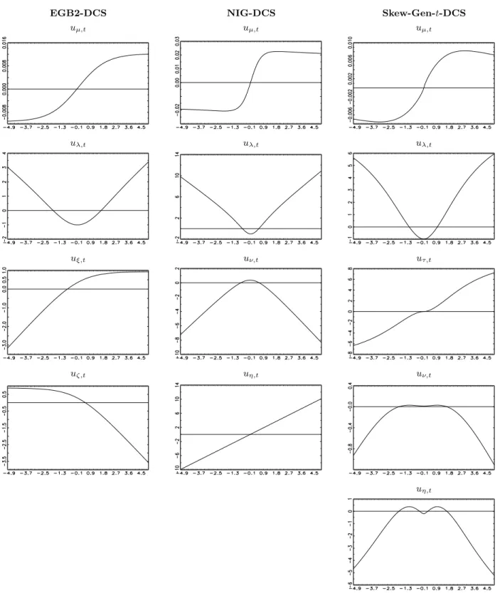
Several specifications in DCS models are robust to extreme observations, because the score functions in those models reduce the effects of outliers (e.g. Harvey, 2013). This property is studied here for the DCS models with dynamic shape parameters. By using the S&P 500 dataset, the outlier transformation of the score functions is presented in Fig. 2, which shows that extreme observations are never accentuated by the score functions of the new DCS models. Therefore, outliers appear within the unexpected return vtrather than within the score functions that update the dynamic equations. 2.2. Model specification test
For the EGB2 and NIG distributions, the first four moments exist. For the Skew-Gen-t distribution, the degrees of freedom parameter specification ensures that the first four moments exist (i.e. the degrees of freedom parameter is>4). The first four conditional moments oftfor the EGB2, NIG and
Skew-Gen-tdistributions are reported in Appendix A. Define the auxiliary error term as:
∗t = t−E(t|Ft−1; Θ) Var1/2(t|Ft−1; Θ)
= t−E(t|1, . . . , t−1; Θ)
Var1/2(t|1, . . . , t−1; Θ)
(2.5)
This transformation reduces the importance of those outliers that appear withint. The robustness of
model specification tests is increased when residuals are standardized according to Eq. (2.5) (see Li, 2004, Chapter 4). The model specification test of the present paper uses the following properties:
E(∗t|Ft−1; Θ) =E(∗t| ∗ 1, . . . , ∗ t−1; Θ) = 0 (2.6) E[(∗t)2−1|Ft−1; Θ] =E[(∗t)2−1|∗1, . . . , ∗t−1; Θ] = 0 (2.7) E[(∗t)3−Skew(t|Ft−1)|Ft−1; Θ] = (2.8) =E[(∗t)3−Skew(t|Ft−1)|∗1, . . . , ∗t−1; Θ] = 0 E[(∗t)4−Kurt(t|Ft−1)|Ft−1; Θ] = (2.9) =E[(∗t)4−Kurt(t|Ft−1)|∗1, . . . , ∗t−1; Θ] = 0
Within the expectations of Eqs. (2.6) to (2.9), the variables are martingale difference sequences (MDSs). The MDS test with optimal lag-order selection (Escanciano and Lobato, 2009) is applied in the present paper, to verify the correct specification for each probability distribution.
3. Statistical inference
All models of this paper are estimated by using the ML method. Blasques et al. (2017, 2018) present the conditions for the asymptotic properties of ML for DCS models with one score-driven parameter. In the present paper, the same conditions are presented for DCS models with several score-driven parameters. The ML estimator is
ˆ ΘML= arg max Θ LL(y1, . . . , yT; Θ) = arg maxΘ 1 T T X t=1 lnf(yt|Ft−1; Θ) (3.1)
where Θ = (Θ1, . . . ,ΘK)0 is the vector of parameters and lnf(yt|Ft−1; Θ) is presented in Appendix A. The following assumptions are used: (A1) f(yt|Ft−1; Θ) = p0(yt|Ft−1; Θ0) for some Θ from the pa-rameter set ˜Θ, where p0 is the true conditional density and Θ0 denotes the true values of the pa-rameters. (A2) RIRf(yt|Ft−1; Θ)dyt = 1 for all yt and Θ. (A3) ˜Θ ∈ IRK is compact. (A4) ˆΘML
is a unique solution to the problem of Eq. (3.1). (A5) LL(·; Θ) is a Borel measurable function on IRT. (A6) For each (y1, . . . , yT) ∈ IRT, LL(y1, . . . , yT;·) is a continuous function on ˜Θ. (A7)
|LL(y1, . . . , yT; Θ)| < b(y1, . . . , yT) for all Θ and E[b(y1, . . . , yT)] < ∞. Under (A1) to (A7), the ML
estimator is consistent: ˆΘML→pΘ0 asT → ∞.
The following results use some additional assumptions: (A8) Θ0 is an interior point within ˜Θ∈IRK. (A9) LL(y1, . . . , yT; Θ) is twice continuously differentiable on all of the interior points of ˜Θ. (A10)
∂[R
IRf(yt|Ft−1; Θ)dyt]/∂Θ = R
IR[∂f(yt|Ft−1; Θ)/∂Θ]dyt.
TheT ×K matrix of contributions to the gradientG(y1, . . . , yT,Θ) is defined by its elements:
Gti(Θ) =
∂lnf(yt|Ft−1; Θ)
∂Θi
(3.2)
for period t= 1, . . . , T and parameteri= 1, . . . , K. Denote thet-th row of G(y1, . . . , yT,Θ) by using
Gt(Θ), which is the score vector for the t-th observation. Under (A1) to (A10), the ML estimator of
Eq. (3.1) is equivalent to the following representation:
1 T T X t=1 Gt( ˆΘML)0 = 1 T T X t=1 Gt1( ˆΘML) .. . GtK( ˆΘML) = 1 T T X t=1 ∂lnf(yt|Ft−1;p0,ΘˆML) ∂Θ1 .. . ∂lnf(yt|Ft−1;p0,ΘˆML) ∂ΘK = 0K×1 (3.3)
According to the mean-value expansion about Θ0: 1 T T X t=1 Gt( ˆΘML)0 = 1 T T X t=1 Gt(Θ0)0+ 1 T " T X t=1 Ht( ¯Θ) # ( ˆΘML−Θ0) (3.4)
where each row of theK×K Hessian matrix
Ht(Θ) =
∂2lnf(yt|Ft−1; Θ)
∂ΘΘ0 (3.5)
which is evaluated atK different mean values, indicated by ¯Θ. Each ¯Θ is located between Θ0 and ˆΘML that is formally expressed as: ||Θ¯ −Θ0|| ≤ ||ΘˆML−Θ0||, where|| · || is the Euclidean norm.
The following results use some additional assumptions: (A11) ∂[R
IRGt(Θ) 0f(y t|Ft−1; Θ)dyt]/∂Θ = R IR[∂Gt(Θ) 0f(y
t|Ft−1; Θ)/∂Θ]dyt. (A12) The information matrixI(Θ0) ≡ −E[Ht(Θ0)] is positive def-inite. (A13) The elements of I(Θ0) are bounded in absolute value by functionb(y1, . . . , yT) for all Θ
and E[b(y1, . . . , yT)]<∞. The conditions of (A13) are studied in Section 3.1. Under (A1) to (A13),
theK×K contribution to the information matrix for periodtis given by:
It(Θ0) =−E[Ht(Θ0)|Ft−1] =E[Gt(Θ0)0Gt(Θ0)|Ft−1] (3.6)
which is evaluated at the true values of parameters. From Eqs. (3.3) and (3.4):
√ T( ˆΘML−Θ0) = " −1 T T X t=1 Ht( ¯Θ) #−1" 1 √ T T X t=1 Gt(Θ0)0 # (3.7) √ T( ˆΘML−Θ0) =I−1(Θ0) " 1 √ T T X t=1 Gt(Θ0)0 # + op(1) (3.8)
The following result uses the assumptions: (A14) A central limit theorem is satisfied for Eq. (3.8); (A14) is studied in Section 3.2. (A15) The DCS model is invertible (Blasques et al., 2017, 2018). Under (A1) to (A15), the asymptotic distribution of the ML estimates is given by:
√ T( ˆΘML−Θ0)→dNK 0K×1,I−1(Θ0) as T → ∞ (3.9)
The asymptotic covariance matrix of ˆΘMLis estimated by using [PT
t=1Gt( ˆΘML)
0G
3.1. Conditions of (A13)
For ease of notation, a DCS model with known constant shape parameters is considered first:
yt=µt+ exp(λt)t (3.10)
µt=c+φµt−1+θuµ,t−1 (3.11)
λt=ω+βλt−1+αuλ,t−1 (3.12)
Variablesµt andλtare re-parameterized, by using the unconditional meansE(µt) = ˜c=c/(1−φ) and
E(λt) = ˜ω =ω/(1−β), as follows:
µt= ˜c(1−φ) +φµt−1+θuµ,t−1 (3.13)
λt= ˜ω(1−β) +βλt−1+αuλ,t−1 (3.14)
for which Θ = (˜c, φ, θ,ω, β, α˜ ) and K = 6. This alternative form of the model is used, since the information matrix is simpler under this representation (Harvey, 2013, p. 34). The conditions for the covariance stationarity ofyt are|φ|<1 and|β|<1. These conditions are named as Condition 1.
To study the finiteness of the elements ofI(Θ0), matrixI(Θ0) is expressed as:
I(Θ0) =E[It(Θ0)] =E
E[Gt(Θ0)0Gt(Θ0)|Ft−1] =E[Gt(Θ0)0Gt(Θ0)] (3.15)
In the following, conditions under which all of the elements of E[Gt(Θ0)0Gt(Θ0)]<∞ are presented. The elements ofGt(Θ0)0 are expressed, according to the chain rule, as follows:
Gt(Θ0)0= ∂lnf(yt|Ft−1;Θ0) ∂θ ∂lnf(yt|Ft−1;Θ0) ∂φ ∂lnf(yt|Ft−1;Θ0) ∂˜c ∂lnf(yt|Ft−1;Θ0) ∂α ∂lnf(yt|Ft−1;Θ0) ∂β ∂lnf(yt|Ft−1;Θ0) ∂ω˜ = ∂lnf(yt|Ft−1;Θ0) ∂µt × ∂µt ∂θ ∂lnf(yt|Ft−1;Θ0) ∂µt × ∂µt ∂φ ∂lnf(yt|Ft−1;Θ0) ∂µt × ∂µt ∂˜c ∂lnf(yt|Ft−1;Θ0) ∂λt × ∂λt ∂α ∂lnf(yt|Ft−1;Θ0) ∂λt × ∂λt ∂β ∂lnf(yt|Ft−1;Θ0) ∂λt × ∂λt ∂ω˜ (3.16)
Four panels within the contribution to the information matrix are defined as follows: It(Θ0) =E[Gt(Θ0)0Gt(Θ0)|Ft−1] =E A(3×3) C(3×3) C(3×3) B(3×3) |Ft−1 (3.17)
where in A only the derivatives of µt appear, in B only the derivatives of λt appear, and in C the
derivatives ofµt and λt appear. By using scalars from A,B andC, the following matrix is defined:
Ft= i3 h ∂lnf(yt|Ft−1;Θ0) ∂µt i2 i03 i3 h ∂lnf(yt|Ft−1;Θ0) ∂µt × ∂lnf(yt|Ft−1;Θ0) ∂λt i i03 i3 h∂lnf(y t|Ft−1;Θ0) ∂µt × ∂lnf(yt|Ft−1;Θ0) ∂λt i i03 i3 h∂lnf(y t|Ft−1;Θ0) ∂λt i2 i03 (3.18)
wherei3 is a (3×1) vector of ones, and the contribution to the information matrix can be written as:
It(Θ0) =E(Ft|Ft−1)◦Dt(Θ0) =E(Ft|Ft−1)◦ ˜ A(3×3) C˜(3×3) ˜ C(3×3) B˜(3×3) (3.19)
where◦ denotes the Hadamard product, and Dt(Θ0) is the outer product of:
˜
Dt= [(∂µt/∂θ),(∂µt/∂φ),(∂µt/∂c˜),(∂λt/∂α),(∂λt/∂β),(∂λt/∂ω˜)] (3.20)
with itself, i.e. Dt(Θ0) = ˜Dt0D˜t; in panel ˜A only the derivatives of µt appear, in panel ˜B only the
derivatives ofλtappear, and in panel ˜C the derivatives of bothµt andλtappear. Dt(Θ0) is not in the conditional expectation in Eq. (3.19), since it is determined byFt−1. I(Θ0) can be written as:
I(Θ0) =E[It(Θ0)] =E(Ft)◦E[Dt(Θ0)] +Mt=E(Ft)◦E ˜ A(3×3) C˜(3×3) ˜ C(3×3) B˜(3×3) +Mt (3.21)
whereMt (K×K) includes the covariances between the elements ofFt and Dt(Θ0).
In the remainder of this section, the conditions of the finiteness of E(Ft), E[Dt(Θ0)] and Mt are
presented. With respect to the finiteness of E(Ft), matrix Ft can be written as:
Ft= i3(u2µ,t/kt2)i03 i3(uµ,t×uλ,t/kt)i03 i3(uµ,t×uλ,t/kt)i03 i3(u2λ,t)i 0 3 (3.22)
where kt is the time-varying scaling parameter. The form of kt is different for different DCS models.
For example, from Eq. (A.8) of Appendix A, for EGB2-DCS the form ofktis:
∂lnf(yt|Ft−1; Θ0)
∂µt
=uµ,t× {Ψ(1)[exp(ξt)] + Ψ(1)[exp(ζt)]}exp(2λt) =
uµ,t
kt
(3.23)
For kt of NIG-DCS and Skew-Gen-t-DCS, see Eqs. (A.22) and (A.34) in Appendix A, respectively.
Based on Eq. (3.22), it is necessary that the unconditional means of (u2µ,t/k2t),uλ,t2 and (uµ,t×uλ,t/kt)
to be finite. This condition is named as Condition 2.
With respect to the finiteness ofE[Dt(Θ0)], the following equations are used (e.g. Harvey, 2013):
˜ Dt0 = ∂µt ∂θ ∂µt ∂φ ∂µt ∂˜c ∂λt ∂α ∂λt ∂β ∂λt ∂ω˜ = Xµ,t−1×∂µ∂θt−1 +uµ,t−1 Xµ,t−1×∂µ∂φt−1 +µt−1−˜c Xµ,t−1×∂µ∂tc˜−1 + 1−φ Xλ,t−1×∂λ∂αt−1 +uλ,t−1 Xλ,t−1×∂λ∂βt−1 +λt−1−ω˜ Xλ,t−1×∂λ∂tω˜−1 + 1−β (3.24)
where Xµ,t ≡ φ+θ(∂uµ,t/∂µt) and Xλ,t ≡ β +α(∂uλ,t/∂λt). Eq. (3.24) provides the following
conditions for the finiteness ofE[Dt(Θ0)]: For panel ˜A it is necessary thatE(Xµ,t2 )<1 and for panel
˜
B it is necessary thatE(X2
λ,t)<1 (for these results, see Harvey, 2013). With respect to panel ˜C, it is
necessary that|E(Xµ,tXλ,t)|<1 (see the proof in Appendix B). In addition, for the DCS model with
score-driven µt and λt, it is also necessary that: (i) the unconditional means of Xµ,t, Xλ,t, uµ,t and
uλ,t are finite, and that the unconditional mean of each product that is formed by all possible pairs of
those variables is also finite (see the proof in Appendix B); (ii) the unconditional second moment of each element of the outer product of the vector (Xµ,t, Xλ,t, uµ,t, uλ,t) with itself is finite (see the proof
in Appendix B). With respect to the latter point, it is noteworthy that the first four moments of t
are finite for all DCS models of this paper. These conditions are named as Condition 3.
With respect to the finiteness of the covariances withinMt, which represent the covariances between
the elements ofFtandDt(Θ0), it is required that the second moments of all variables in the covariances are finite. The variables in the covariances can be seen in Eqs. (3.22) and (3.24). The covariances between the elements of Ft and Dt(Θ0) are finite under Condition 3.
3.2. Conditions of (A14)
By using Eq. (3.8), the following result is equivalent to Eq. (3.9):
T−1/2
T
X
t=1
Gt(Θ0)0 →dNK[0K×1,I(Θ0)] (3.25)
By using the Cram´er-Wold Device (e.g. White, 1984), Eq. (3.25) is true if for all a∈IRK:
a0T−1/2PT
t=1Gt(Θ0)
0
[a0I(Θ0)a]1/2 →dN(0,1) (3.26)
where a is a (K ×1) vector. To show the asymptotic result in Eq. (3.26), for ease of notation
Zt≡a0Gt(Θ0)0 is introduced and Definition 5.15 and Theorem 5.16 from the work of White (1984) are used. According to those two theorems, if (E1) Zt is stationary and ergodic, (E2) E(Zt2) < ∞, and
(E3) Ztis an adapted mixingale (with respect to this last point, see Hamilton, 1994, p. 190):
E[E(Zt|Ft−m)2]
1/2
=E|E(Zt|Ft−m)| ≤ctγm asm→ ∞ and γm →0 (3.27)
whereFt−m has started in the infinite past and is available until periodt−m(including periodt−m),
ct is a finite non-negative sequence and γm =O[1/(m1+ε)] forε >0, then Eq. (3.26) holds.
The proof of Eq. (3.26) uses the following condition: Condition 4 is that t is stationary and
ergodic. (E1) can be shown as follows: Theorem 3.35 of White (1984) shows that a measurable function transforms stationary and ergodic variables into stationary and ergodic variables. The transformations oftinZt=a0Gt(Θ0)0satisfy the conditions of that theorem under (A1) to (A13) and Conditions 1 to 4. The results of Brandt (1986) and Diaconis and Freedman (1999) on stochastic recurrence equations (SREs) support this conclusion. In relation to those results, Eq. (3.24) can be written as:
∂µt ∂θ ∂µt ∂φ ∂µt ∂˜c ∂λt ∂α ∂λt ∂β ∂λt ∂ω˜ = Xµ,t−1 0 0 0 0 0 0 Xµ,t−1 0 0 0 0 0 0 Xµ,t−1 0 0 0 0 0 0 Xλ,t−1 0 0 0 0 0 0 Xλ,t−1 0 0 0 0 0 0 Xλ,t−1 ∂µt−1 ∂θ ∂µt−1 ∂φ ∂µt−1 ∂c˜ ∂λt−1 ∂α ∂λt−1 ∂β ∂λt−1 ∂ω˜ + uµ,t−1 µt−1−c˜ 1−φ uλ,t−1 λt−1−ω˜ 1−β (3.28)
and the following compact notation is used for the previous equation: ˜ Dt0 =A∗t−1D˜ 0 t−1+B ∗ t−1 (3.29)
which is a SRE. Under (A1) to (A13), Conditions 1 to 4 and by using Theorem 3.35 of White (1984),
A∗t−1andBt∗−1are stationary and ergodic. Moreover, fromE(Xµ,t2 )<1 andE(Xλ,t2 )<1 of Condition 3 and by using the Cauchy–Schwarz inequality: |E(Xµ,t)|<1 and|E(Xλ,t)|<1 in Eq. (3.28). By using
the results of Brandt (1986) and Diaconis and Freedman (1999), ˜Dt0 is stationary and ergodic. Under (A1) to (A13), Conditions 1 to 4 and Theorem 3.35 of White (1984), Zt=a0Gt(Θ0)0 is also stationary
and ergodic. (E2) can be shown as follows:
E(Zt2) =E{[a0Gt(Θ0)0]2}= Var[a0Gt(Θ0)0] +E2[a0Gt(Θ0)0] = (3.30)
a0Var[Gt(Θ0)0]a+{a0E[Gt(Θ0)0]}2 =a0E[Gt(Θ0)0Gt(Θ0)]a=a0I(Θ0)a <∞
whereE[Gt(Θ0)0] = 0 and the finiteness of I(Θ0) are used under (A1) to (A13) and Conditions 1 to 4. According to (E3), the m-step ahead forecast E(Zt|Ft−m) converges in absolute expected value
to the unconditional mean of zero as m → ∞(Hamilton, 1994). This can be shown as follows: The unconditional mean of Zt is zero, because E(Zt) =E[a0Gt(Θ0)0] =a0E[Gt(Θ0)0] = a00K×1 = 0 under (A1) to (A13) and Conditions 1 to 4. Moreover, Eq. (3.16) shows that Gt(Θ0)0 is the Hadamard
product of a K×1 vector of the score functions and ˜D0t. Under (A1) to (A13) and Conditions 1 to 4, the conditional and unconditional means of the score functions are zero. Therefore, the m-step ahead forecasts of the score functions converge to zero as m → ∞. Under the same conditions, Lemma 6 (Harvey, 2013, p. 36) is applied to ˜Dt0, which provides the following forecasting results:
lim m→∞E ∂µt ∂θ |Ft−m = lim m→∞E ∂µt ∂φ|Ft−m = 0 (3.31) lim m→∞E ∂λt ∂α|Ft−m = lim m→∞E ∂λt ∂β|Ft−m = 0 (3.32) lim m→∞E ∂µt ∂˜c|Ft−m = 1−φ 1−E(Xµ,t) (3.33)
lim m→∞E ∂λt ∂ω˜|Ft−m = 1−β 1−E(Xλ,t) (3.34)
The forecasts of Eqs. (3.31) and (3.32) converge to zero and the forecasts of Eqs. (3.33) and (3.34) converge to a non-zero constant. As a consequence limm→∞E[Gt(Θ0)0|Ft−m] = 0,
lim m→∞E[Zt|Ft−m] = limm→∞E[a 0 Gt(Θ0)0|Ft−m] = lim m→∞a 0 E[Gt(Θ0)0|Ft−m] = 0 (3.35)
which implies that E|E(Zt|Ft−m)| ≤ctγm asm→ ∞ and γm →0. 3.3. The asymptotic properties of ML for two models
Proposition 1: For Eqs. (3.10) to (3.12), √T( ˆΘML−Θ0) →d N[0K×1,I−1(Θ0)] as T → ∞, under
(A1) to (A15) and the following conditions: Condition 1 is that|φ|<1 and|β|<1. Condition 2 is that
E(u2µ,t/kt2),E(u2λ,t) andE(uµ,t×uλ,t/kt) are finite. Condition 3 is that E(Xµ,t2 )<1,E(Xλ,t2 )<1 and
|E(Xµ,tXλ,t)|<1, whereXµ,t =φ+θ(∂uµ,t/∂µt) andXλ,t=β+α(∂uλ,t/∂λt). Condition 3 also requires
that: (i) the unconditional means ofXµ,t,Xλ,t,uµ,tanduλ,tare finite, and that the unconditional mean
of each product that is formed by all possible pairs of those variables is also finite; (ii) the unconditional second moment of each element of the outer product of the vector (Xµ,t, Xλ,t, uµ,t, uλ,t) with itself is
finite. Condition 4 is thatt is strictly stationary and ergodic.
Conditions 1 to 4 can be extended to DCS models with score-driven shape parameters. For example, the following EGB2-DCS model witht∼EGB2[0,1,exp(ξt),exp(ζt)] is considered:
yt=µt+ exp(λt)t (3.36)
µt=c+φµt−1+θuµ,t−1 (3.37)
λt=ω+βλt−1+αuλ,t−1 (3.38)
ξt=δ1+γ1ξt−1+κ1uξ,t−1 (3.39)
ζt=δ2+γ2ζt−1+κ2uζ,t−1 (3.40)
Proposition 2: For Eqs. (3.36) to (3.40), √T( ˆΘML−Θ0) →d N[0K×1,I−1(Θ0)] as T → ∞, under
(A1) to (A15) and the following conditions: Condition 1 is that |φ| < 1, |β| < 1, |γ1| < 1 and |γ2|<1. Condition 2 is thatE(u2µ,t/kt2),E(u2λ,t),E(u2ξ,t), E(u2ζ,t),E(uµ,t×uλ,t/kt),E(uµ,t×uξ,t/kt),
E(uµ,t×uζ,t/kt),E(uλ,t×uξ,t),E(uλ,t×uζ,t), andE(uξ,t×uζ,t) are finite. Condition 3 is thatE(Xµ,t2 )<
1, E(Xλ,t2 ) < 1, E(Xξ,t2 ) < 1, E(Xζ,t2 ) < 1, |E(Xµ,tXλ,t)| < 1, |E(Xµ,tXξ,t)|< 1, |E(Xµ,tXζ,t)| < 1,
|E(Xλ,tXξ,t)| < 1, |E(Xλ,tXζ,t)| < 1 and |E(Xξ,tXζ,t)| < 1, where Xµ,t = φ+θ(∂uµ,t/∂µt), Xλ,t =
β+α(∂uλ,t/∂λt), Xξ,t =γ1+κ1(∂uξ,t/∂ξt) and Xζ,t=γ2+κ2(∂uζ,t/∂ζt). Condition 3 also requires
that: (i) the unconditional means of Xµ,t, Xλ,t, Xξ,t, Xζ,t, uµ,t, uλ,t, uξ,t and uζ,t are finite, and
that the unconditional mean of each product that is formed by all possible pairs of those variables is also finite; (ii) the unconditional second moment of each element of the outer product of the vector (Xµ,t, Xλ,t, Xξ,t, Xζ,t, uµ,t, uλ,t, uξ,t, uζ,t) with itself is finite. Condition 4 is thatt is strictly stationary
and ergodic.
3.4. MC simulation experiments
For all MC experiments, zero mean µt= 0, unit scale exp(λt) = 1, and score-driven shape parameters
are used for t = 1, . . . , T. Two sets of true parameter values are used: The first set assumes high persistence for the shape parameters (i.e. γk=0.95 for all k). The second set assumes low persistence
for the shape parameters (i.e. γk=0.15 for all k). The true values of all parameters are presented
in Table 1. By using those true values, 1,000 trajectories are simulated and each trajectory includes
T = 10,000 periods. With respect to the sample size T, it is noteworthy that DCS models with dynamic shape need a large sample size for the reliable estimation of tail shape dynamics.
By using the ML method, the parameters of the DCS models with dynamic shape parameters are estimated for each trajectory. In Table 1, the 5%, 50% and 95% quantiles of the 1,000 parameter estimates are reported. For the high-persistence case, the medians give a good approximation of the true values and the 90% confidence intervals of the quantiles include all true values. For the low-persistence case, the medians give a good approximation of most of the true values; the only exceptions are some of the constant parameters, for which the true value is not within the 90% confidence interval (e.g. δ2 for EGB2-DCS and NIG-DCS). The 90% confidence intervals also show that the ML estimation is more precise for the high persistence case than it is for the low persistence case. The medians indicate that dynamic parameter γk and parameters of the score functions κk are precisely estimated for all
cases.
4. Data
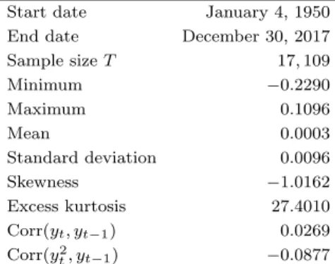
Daily data are used from the closing prices of the S&P 500 indexptfor the period of January 4, 1950 to
S&P 500ytare presented, where yt= ln(pt/pt−1) fort= 1, . . . , T and pre-sample data are used forp0. The following results can be highlighted: The negative skewness estimate indicates that the mass of the distribution ofytis concentrated on the right side, and the high excess kurtosis estimate suggests
heavy tails of yt. The negative correlation coefficient Corr(yt2,yt−1) suggests that high volatility often follows significant negative returns, which motivates the consideration of leverage effects withinλt. The
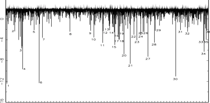
evolution of yt is presented in Fig. 3, where extreme observations are indicated by using the µ±5σ
interval; µ and σ are the estimates of mean and standard deviation, respectively. In the same figure, the concentration of outliers during the period of the 2008 US financial crisis can be observed.
5. Empirical results
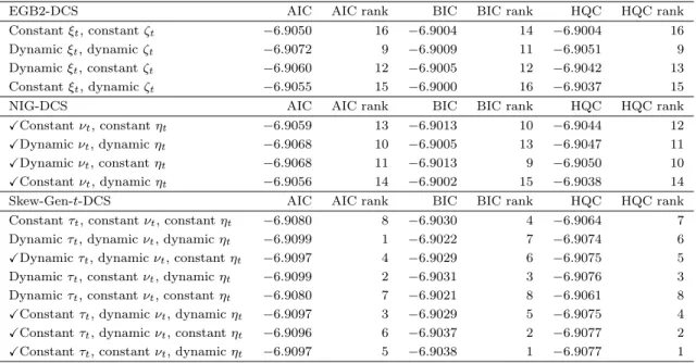
In this section, the ML estimation results for the S&P 500 are presented for the EGB2-DCS (Table 3), NIG-DCS (Table 4) and Skew-Gen-t-DCS (Tables 5(a) and (b)) models. LL-based performances of those models are compared in Table 6. The evolutions of ρk,t and λt are presented for all models in
Figs. 4, 5, 6(a) and 6(b). The dates of some extreme events are highlighted in Fig. 7.
Tables 3 to 5 show the following results: For most of the specifications,φparameter which measures the persistence of conditional location is significantly different from zero. The scaling parameter of the score function with respect to location θ is positive and significant for all models. For all of the specifications, highly significant ω, α, α∗ and β parameters are found for the scale. For most of the specifications, the dynamic parameters of shape (i.e. γ1, γ2 and γ3) are significant and positive. For all of the specifications, the scaling parameter of the score function with respect to shape (i.e. κ1, κ2 and κ3) is significantly different from zero (i.e. the DCS models are identified; Harvey, 2013).
All estimates of φ, β, γ1, γ2 and γ3 are less than one in absolute value (Tables 3 to 5). Thus, Condition 1 is supported. In Tables 3 to 5, the estimates of Cµ = E(Xµ,t2 ), Cλ = E(Xλ,t2 ), Cρ,1 =
E(Xρ,21,t), Cρ,2 =E(Xρ,22,t), Cρ,3 =E(Xρ,23,t), Cµ,λ = |E(Xµ,tXλ,t)|, Cµ,ρ,1 =|E(Xµ,tXρ,1,t)|, Cµ,ρ,2 =
|E(Xµ,tXρ,2,t)|, Cµ,ρ,3 = |E(Xµ,tXρ,3,t)|, Cλ,ρ,1 = |E(Xλ,tXρ,1,t)|, Cλ,ρ,2 = |E(Xλ,tXρ,2,t)|, Cλ,ρ,3 = |E(Xλ,tXρ,3,t)|,Cρ,1,ρ,2=|E(Xρ,1,tXρ,2,t)|,Cρ,1,ρ,3 =|E(Xρ,1,tXρ,3,t)|andCρ,2,ρ,3 =|E(Xρ,2,tXρ,3,t)|are
also reported. All of those estimates are less than one. Thus, the corresponding formulas of Condition 3 are supported for the ML estimates. For the variables of Conditions 2 and 3, the augmented Dickey– Fuller (1979) (hereinafter, ADF) unit root test with constant is performed, which supports those conditions. Condition 4 is a maintained assumption in this paper.
Tables 3 to 5. For EGB2-DCS, the MDS null hypothesis of the Escanciano–Lobato test is rejected for all specifications, with respect to skewness and kurtosis. For NIG-DCS, the MDS null hypothesis of the Escanciano–Lobato test is never rejected. For Skew-Gen-t-DCS, eight different specifications with respect to dynamic versus constant shape are considered, and for four out of eight specifications the MDS null hypothesis of the Escanciano–Lobato test is not rejected up to the fourth moment.
In-sample model performances are compared by using the following metrics: LL, Akaike informa-tion criterion (AIC), Bayesian informainforma-tion criterion (BIC), Hannan-Quinn criterion (HQC), and the likelihood-ratio (LR) test (Tables 3 to 6). For those metrics, the statistical performance of at least one of the DCS specifications with dynamic shape parameters is superior to the statistical performance of the DCS model with constant shape parameters. For the LR test, at least one of the DCS specifications with dynamic shape parameters is significantly superior to the nested DCS specification with constant shape parameters. The results also suggest that the statistical performance of the Skew-Gen-t-DCS model is superior to the statistical performances of the EGB2-DCS and NIG-DCS models.
The evolutions ofρk,tandλtare presented in Figs. 4 to 6. Those figures indicate that: (i) the shape
parameters are time-varying for all models; (ii) for the DCS specifications with dynamic shape, the shape parameters identify the dates of outliers. As an example, in Fig. 7, the identification of outliers is studied for DCS-Skew-Gen-t with constant τt, dynamic νt and constant ηt. In that figure, some
numbers indicate those trading days when νt is relatively low, which suggests that the probability of
there being an outlier is relatively high. Important events are reported in Appendix C for those trading days that are indicated in Fig. 7. Those events may have significantly impacted the US stock market.
6. VaR backtesting
In this section VaR backtesting applications are presented, in which the VaR measurements of the DCS models with constant and dynamic shape parameters are compared. The results provide the following insight for practitioners about the quality of VaR measurement for the new DCS specifications: The DCS models with dynamic shape effectively predict consecutive additive outliers, while the DCS models with constant shape fail to predict the second outlier.
As aforementioned, extreme observations in the S&P 500 log-returns are concentrated during the period of the 2008 US financial crisis (Fig. 3). This motivates the consideration of the period of September 2, 2008 to March 31, 2009 (i.e. 146 trading days) in the VaR backtesting applications. During that period there were 24 outliers (Fig. 3). The design of the VaR backtesting procedure
of this paper is according to the approach of the Basel Committee (1996), in which a 1-day VaR is estimated out-of-sample at the 99% confidence level for each of the most recent 250 trading days. In the present paper, a VaR(1 day, 99%) is estimated for each of the 146 days of the backtesting period. A rolling-window estimation approach is used for all DCS models, and 10,000 observations are included into each rolling window. As alternatives, the use of 2,500 and 5,000 observations is also considered for the rolling windows, but more robust ML estimates are obtained forT = 10,000. VaR is approximated after the parameter estimation by using MC simulation, for which 100,000 possible log-returns are simulated for the trading day after the last observation of each rolling window. VaR(1 day, 99%) is defined by the 1% quantile of the log-return simulations. The performance of VaR is compared for the following models: (i) EGB2-DCS with constant and dynamic shape parameters; (ii) NIG-DCS with constant and dynamic shape parameters; (iii) Skew-Gen-t-DCS with constant and dynamic shape parameters. All shape parameters are time-varying for the DCS specifications with dynamic shape parameters.
One of the backtests that are suggested by the Basel Committee (1996) is the ‘traffic light approach’, which is based on the number of those trading days during the period defined by the last 250 trading days, for which the realized return is lower than the VaR estimate. That number represents the ‘VaR failures’ during the backtesting period. In the present paper, the VaR failures for the 146-day backtesting period are counted in a similar way. Furthermore, the test of Kupiec (1995) is also applied to evaluate whether the proportion of VaR(1 day, 99%) failures is significantly higher than 1% during the backtesting period. The null hypothesis of the Kupiec test is that the VaR model is appropriate.
The number of VaR failures and the Kupiec test results for the 146-day backtesting period are presented in Table 7(a). The number of VaR failures does not differ for the DCS specifications with constant and dynamic shape. For EGB2-DCS, 4 VaR failures are found for both the constant- and dynamic-shape models. The results also show that VaR for EGB2-DCS is inappropriate according to the Kupiec test, at the 10% level of significance. For NIG-DCS and Skew-Gen-t-DCS, 2 VaR failures are found for both the constant- and dynamic-shape models, and the Kupiec test results support the quality of VaR measurements. Conclusions from Table 7(a): (i) the DCS models with dynamic shape parameters do not provide better VaR measurements than the DCS models with constant shape parameters for the backtesting period of the S&P 500; (ii) the VaR measurements for the NIG-DCS and Skew-Gen-t-DCS models are superior to the VaR measurement for the EGB2-DCS model.
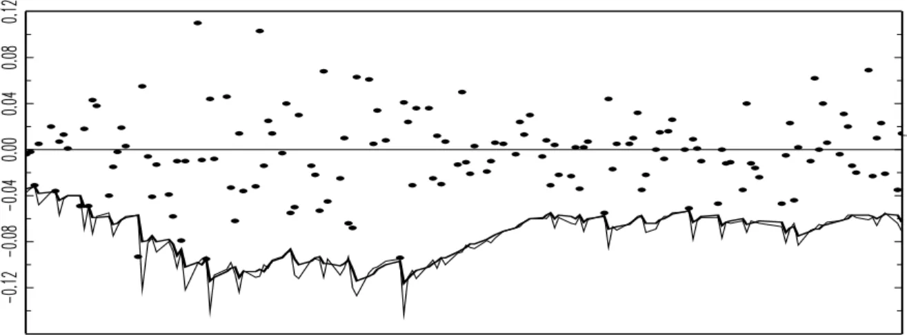
To provide a further analysis of VaR, the evolution of S&P 500 log-returns and the evolution of the VaR estimates are presented for all models in Fig. 8. That figure provides the following interesting insight. It shows that, after each extreme observation, the predicted potential extreme loss of the next day is higher for the DCS specification with dynamic shape parameter than for the DCS specification with constant shape parameter. This result is robust, because it is obtained for the EGB2, NIG and Skew-Gen-tdistributions, and it provides the following intuition: If outliers occur on consecutive trading days, then: (i) the VaR measurements for DCS models with constant shape parameters may fail for the second outlier; (ii) the VaR measurements for DCS models with dynamic shape parameters will detect the second outlier. The correct detection of consecutive additive outliers is important in the VaR backtesting literature, and it motivated the work of Christofferssen (1998). The null hypothesis of the Christofferssen test is that the arrival times of VaR failures are independent. If that null hypothesis is rejected, for example, due to consecutive VaR failures within the backtesting period, then the econometric model is not updated correctly after extreme observations.
To study the issue of consecutive outliers, a modified S&P 500 dataset is used for the backtesting period. For each of those days when the VaR fails (see the dates in Table 7(a)), the outlier is duplicated for the next day. The results for the 146-day backtesting period are presented in Table 7(b). For EGB2-DCS, 3 VaR failures are found for both the constant- and dynamic-shape models. Although the number of VaR failures is identical for both models, two of those VaR failures are on consecutive trading days for the constant-shape model, while the three VaR failures are on non-consecutive trading days for the dynamic-shape model. For NIG-DCS and Skew-Gen-t-DCS, 3 VaR failures are found for the constant-shape models and 2 VaR failures are found for the dynamic-shape models. It is important to highlight that consecutive VaR failures are observed for all DCS models with constant shape parameters, while the VaR failures are never on consecutive days for the DCS models with dynamic shape parameters. The VAR backtesting application indicates that, during periods of high market volatility, the VaR measurements of DCS models with dynamic shape parameters are protected against consecutive additive outliers, but the VaR measurements of DCS models with constant shape parameters fail on the trading day of the second additive outlier.
7. Conclusions
In this paper, new score-driven models with dynamic shape parameters have been suggested, which improve the performance of the score-driven models with constant shape parameters, since: (i) they
have superior in-sample statistical performances, and (ii) they provide more accurate out-of-sample VaR measurements. Log-return time series data have been used from the S&P 500 index for the period of 1950 to 2017. All DCS models have been estimated by using the ML method, the conditions of the asymptotic properties of the ML estimator have been provided, and the use of the ML estimator has been supported by performing MC simulation experiments. The in-sample statistical performances of DCS models with dynamic shape parameters have been superior to the in-sample statistical per-formances of DCS models with constant shape parameters. VaR backtesting for a period during the 2008 US financial crisis has indicated that the DCS models with dynamic shape parameters effectively predict extreme losses for consecutive additive outliers, while the DCS models with constant shape parameters are incorrectly updated after the first outlier and fail to predict extreme losses for the second outlier. The in-sample statistical performance and out-of-sample VAR backtesting results of this paper may motivate the consideration of DCS models with dynamic shape parameters in the VaR measurement practices of financial risk managers for periods of high market volatility.
Acknowledgments
Previous versions of this paper were presented at the GESG Research Seminar (Universidad Francisco Marroqu´ın, March 7, 2019), Cambridge-INET Conference on Score-Driven and Nonlinear Time Series Models (University of Cambridge, March 27-29, 2019), and IX-th Workshop in Time Series Econo-metrics (University of Zaragoza, April 4-5, 2019). The authors are thankful to Matthew Copley, Juan Carlos Escanciano, Andrew Harvey, Jason Jones and to all seminar and conference participants for the helpful comments and suggestions. Astrid Ayala and Szabolcs Blazsek acknowledge funding from the School of Business of Universidad Francisco Marroqu´ın. Alvaro Escribano acknowledges funding from the Spanish Ministry of Economy, Industry and Competitiveness (ECO2015-68715-R, ECO2016-00105-001), Consolidation Grant (#2006/04046/002), and Maria de Maeztu Grant (MDM 2014-0431).
References
Backus, D., Chernov, M., Martin, I., 2011. Disasters implied by equity index options. Journal of Finance 66 (6): 1969–2012. doi: 10.1111/j.1540-6261.2011.01697.x.
Bakshi, G., Kapadia, N., Madan D., 2003. Stock return characteristics, skew laws, and the differential pricing of individual equity options. Review of Financial Studies 16 (1): 101–143. doi: 10.1093/rfs/16.1.0101.
Barndorff-Nielsen, O., Halgreen, C., 1977. Infinite divisibility of the hyperbolic and generalized inverse Gaussian distri-butions. Probability Theory and Related Fields 38 (4): 309–311. doi: 10.1007/bf00533162.
Barndorff-Nielsen, O., Shephard, N., 2002. Econometric analysis of realized volatility and its use in estimating stochastic volatility models. Journal of the Royal Statistical Society: Series B (Statistical Methodology) 64 (2): 253–280. doi: 10.1111/1467-9868.00336.
Basel Committee, 1996. Supervisory framework for the use of “backtesting” in conjunction with the internal models approach to market risk capital requirements. Available at www.bis.org.
Blasques, F., Koopman, S.J., Lucas, A., 2015. Information-theoretic optimality of observation-driven time series models for continuous responses. Biometrika 102 (2): 325–343. doi: 10.1093/biomet/asu076.
Blasques, F., Koopman, S.J., Lucas, A., 2017. Maximum likelihood estimation of score-driven models. TI 2014-029/III, Tinbergen Institute Discussion Paper. https://papers.tinbergen.nl/14029.pdf.
Blasques, F., Gorgi, P., Koopman, S.J., Wintenberger, O., 2018. Feasible invertibility conditions and maximum likelihood estimation for observation-driven models. Electronic Journal of Statistics 12 (1): 1019–1052. doi: 10.1214/18-EJS1416.
Blazsek, S., Ho, H.-C., Liu, S.-P., 2018. Score-driven Markov-switching EGARCH models: an application to systematic risk analysis. Applied Economics 50 (56): 6047–6060. doi: 10.1080/00036846.2018.1488073.
Bollerslev, T., 1986. Generalized autoregressive conditional heteroskedasticity. Journal of Econometrics 31 (3): 307–327. doi:10.1016/0304-4076(86)90063-1.
Bollerslev, T., 1987. A conditionally heteroscedastic time series model for speculative prices and rates of return. The Review of Economics and Statistics 69 (3): 542–547. doi: 10.2307/1925546.
Bollerslev, T., Tauchen, G., Zhou, H., 2009. Expected stock returns and variance risk premia. Review of Financial Studies 22 (11): 4463–4492. doi: 10.1093/rfs/hhp008.
Bollerslev, T., Todorov, V., 2011. Estimation of jump tails. Econometrica 79 (6): 1727–1783. doi: 10.3982/ECTA9240. Bollerslev, T., Todorov, V., 2014. Time-varying jump tails. Journal of Econometrics 183 (2): 168–180.
doi: 10.1016/j.jeconom.2014.05.007.
Bollerslev, T., Todorov, V., Xu, L., 2015. Tail risk premia and return predictability. Journal of Financial Economics 118 (1): 113–134. doi: 10.1016/j.jfineco.2015.02.010.
Brandt, A., 1986. The stochastic equation Yn+1 = AnYn+Bn with stationary coefficients. Advances in Applied Probability 18 (1): 211–220. doi: 10.2307/1427243.
Caivano, M., Harvey, A.C., 2014. Time-series models with an EGB2 conditional distribution. Journal of Time Series Analysis 35 (6): 558–571. doi: 10.1111/jtsa.12081.
Christofferssen, P., 1998. Evaluating interval forecasts. International Economic Review 39(4): 841–862. doi: 10.2307/2527341.
Creal, D., Koopman, S.J., Lucas, A., 2011. A dynamic multivariate heavy-tailed model for time-varying volatilities and correlations. Journal of Business & Economic Statistics 29 (4): 552–563.
doi: 10.1198/jbes.2011.10070.
Creal, D., Koopman, S.J., Lucas, A., 2013. Generalized autoregressive score models with applications. Journal of Applied Econometrics 28 (5): 777–795. doi: 10.1002/jae.1279.
Diaconis, P., Freedman, D., 1999. Iterated random functions. SIAM Review 41 (1): 45–76. doi: 10.1137/S0036144598338446.
Dickey, D.A., Fuller, W.A., 1979. Distribution of the estimators for autoregressive time series with a unit root. Journal of the American Statistical Association 74 (366): 427–431. doi: 10.2307/2286348.
Engle, R.F., 1982. Autoregressive conditional heteroscedasticity with estimates of the variance of United Kingdom inflation. Econometrica 50 (4): 987–1008. doi: 10.2307/1912773.
Escanciano, J.C., Lobato, I.N., 2009. An automatic Portmanteau test for serial correlation. Journal of Econometrics 151 (2): 140–149. doi: 10.1016/j.jeconom.2009.03.001.
Galbraith, J.W., Zernov, S., 2004. Circuit breakers and the tail index of equity returns. Journal of Financial Economet-rics 2 (1): 109–129. doi: 10.1093/jjfinec/nbh005.
Hamilton, J.D., 1994. Time Series Analysis. Princeton University Press, Princeton.
Harvey, A.C., 1989. Forecasting, Structural Time Series Models and the Kalman Filter. Cambridge University Press, Cambridge.
Harvey, A.C., 2013. Dynamic Models for Volatility and Heavy Tails. Cambridge University Press, Cambridge.
Harvey, A.C., Chakravarty, T., 2008. Beta-t-(E)GARCH. Cambridge Working Papers in Economics 0840, Faculty of Economics, University of Cambridge, Cambridge.
http://www.econ.cam.ac.uk/research/repec/cam/pdf/cwpe0840.pdf.
Harvey, A.C., Lange, R.J., 2017. Volatility modeling with a generalized t-distribution. Journal of Time Series Analysis 38 (2): 175–190. doi: 10.1111/jtsa.12224.
Harvey, A.C., Ruiz, E., Shephard, N., 1994. Multivariate stochastic variance models. Review of Economic Studies 61 (2): 247–264. doi: 10.2307/2297980.
Harvey, A.C., Shephard, N., 1996. Estimation of an asymmetric stochastic volatility models for asset returns. Journal of Business & Economic Statistics 14 (4): 429–434. doi: 10.1080/07350015.1996.10524672.
Harvey, A.C., Sucarrat, G., 2014. EGARCH models with fat tails, skewness and leverage. Computational Statistics & Data Analysis 76: 320–338. doi: 10.1016/j.csda.2013.09.022.
Kelly, B., Jiang, H., 2014. Tail risk and asset prices. Review of Financial Studies 27 (10): 2841–2871. doi: 10.1093/rfs/hhu039.
Kib, S., Shephard, N., Chib, S., 1998. Stochastic volatility: likelihood inference and comparison with ARCH models. The Review of Economic Studies 65 (3): 361–393. doi: 10.1111/1467-937X.00050.
Kupiec, P.H., 1995. Techniques for verifying the accuracy of risk measurement models. The Journal of Derivatives 3(2): 73–84. doi: 10.3905/jod.1995.407942.
Li, W.K., 2004. Diagnostic Checks in Time Series. Chapman & Hall/CRC, Boca Raton.
McDonald, J.B., Michelfelder, R.A., 2017. Partially adaptive and robust estimation of asset models: accommodating skewness and kurtosis in returns. Journal of Mathematical Finance 7: 219–237. doi: 10.4236/jmf.2017.71012. Nelson, D.B., 1991. Conditional heteroskedasticity in asset returns: a new approach. Econometrica 59 (2): 347–370.
doi: 10.2307/2938260.
Quintos, C., Fan, Z., Phillips, P.C.B., 2001. Structural change tests in tail behavior and the Asian crisis. The Review of Economic Studies 68 (3): 633–663. doi: 10.1111/1467-937X.00184.
White, H., 1984. Asymptotic Theory for Econometricians. Academic Press, San Diego. Appendix A
In this appendix, for each error specification, the conditional distribution ofyt, the conditional mean ofyt, the conditional volatility ofyt, the log of the conditional density ofyt, the scaled score function for locationuµ,t, and the score functions for scaleuλ,t and shapeuρ,k,tare presented.
(1) For the EGB2-DCS model, t ∼ EGB2[0,1,exp(ξt),exp(ζt)], where both shape parameters are positive. The conditional mean, conditional variance, conditional skewness and conditional kurtosis oftare given by:
E(t|Ft−1; Θ) = Ψ(0)[exp(ξt)]−Ψ(0)[exp(ζt)] (A.1) Var(t|Ft−1; Θ) = Ψ(1)[exp(ξt)] + Ψ(1)[exp(ζt)] (A.2)
Skew(t|Ft−1; Θ) = Ψ(2)[exp(ξt)]−Ψ(2)[exp(ζt)] (A.3)
Kurt(t|Ft−1; Θ) = Ψ(3)[exp(ξt)] + Ψ(3)[exp(ζt)] (A.4)
respectively; Θ is the vector of parameters and Ψ(i)(x) is the polygamma function of orderi. For the EGB2-DCS model,
yt|Ft−1∼EGB2[µt,exp(−λt),exp(ξt),exp(ζt)]. The conditional mean and the conditional volatility ofyt are
E(yt|Ft−1; Θ) =µt+ exp(λt)
n
SD(yt|Ft−1; Θ) = exp(λt){Ψ(1)[exp(ξt)] + Ψ(1)[exp(ζt)]}1/2 (A.6)
respectively. The log of the conditional density ofytis
lnf(yt|Ft−1; Θ) = exp(ξt)t−λt−ln Γ[exp(ξt)]−ln Γ[exp(ζt)] (A.7) + ln Γ[exp(ξt) + exp(ζt)]−[exp(ξt) + exp(ζt)] ln[1 + exp(t)]
The score functions with respect toµt,λt,ξtandζt are as follows. Firstly, the score function with respect toµt is
∂lnf(yt|Ft−1; Θ)
∂µt
=uµ,t× {Ψ(1)[exp(ξt)] + Ψ(1)[exp(ζt)]}exp(2λt) =
uµ,t
kt
(A.8) where
uµ,t={Ψ(1)[exp(ξt)] + Ψ(1)[exp(ζt)]}exp(λt)
[exp(ξt) + exp(ζt)] exp(t)
exp(t) + 1−exp(ξt)
(A.9) is the scaled score function. Secondly, the score function with respect toλtis
uλ,t=
∂lnf(yt|Ft−1; Θ)
∂λt
= [exp(ξt) + exp(ζt)] texp(t)
exp(t) + 1−exp(ξt)t−1 (A.10)
Thirdly, the score function with respect toξt is
uξ,t=
∂lnf(yt|Ft−1; Θ)
∂ξt
= exp(ξt)t−exp(ξt)Ψ(0)[exp(ξt)] (A.11)
+ exp(ξt)Ψ(0)[exp(ξt) + exp(ζt)]−exp(ξt) ln[1 + exp(t)] Fourthly, the score function with respect toζtis
uζ,t=
∂lnf(yt|Ft−1; Θ)
∂ζt
=−exp(ζt)Ψ(0)[exp(ζt)] (A.12)
+ exp(ζt)Ψ(0)[exp(ξt) + exp(ζt)]−exp(ζt) ln[1 + exp(t)]
(2) For the NIG-DCS model,t∼NIG[0,1,exp(νt),exp(νt)tanh(ηt)], where tanh(x) is the hyperbolic tangent function, and the absolute value of parameter exp(νt)tanh(ηt) is less than parameter exp(νt) as required for the NIG distribution. The conditional mean, conditional variance, conditional skewness and conditional kurtosis oft are given by:
E(t|Ft−1; Θ) = tanh(ηt) [1−tanh2(ηt)]1/2 (A.13) Var(t|Ft−1; Θ) = exp(−νt) [1−tanh2(ηt)]3/2 (A.14) Skew(t|Ft−1; Θ) = 3tanh(ηt) exp(νt/2) 1−tanh2(ηt)1/4 (A.15) Kurt(t|Ft−1; Θ) = 3 + 3 1 + 4tanh2(ηt) exp(νt) 1−tanh2(ηt)1/2 (A.16)
respectively. For the NIG-DCS model, the conditional distribution ofyt is
yt|Ft−1 ∼NIG[µt,exp(λt),exp(νt−λt),exp(νt−λt)tanh(ηt)] (A.17)
The conditional mean and the conditional volatility ofytare
E(yt|Ft−1; Θ) =µt+
exp(λt)tanh(ηt)
SD(yt|Ft−1; Θ) = exp(2λt−νt) [1−tanh2(ηt)]3/2 1/2 (A.19) respectively. The log of the conditional density ofytis
lnf(yt|Ft−1; Θ) =νt−λt−ln(π) + exp(νt)[1−tanh2(ηt)]1/2 (A.20) + exp(νt)tanh(ηt)t+ lnK(1) exp(νt) q 1 +2 t −1 2ln(1 + 2 t)
whereK(1)(x) is the modified Bessel function of the second kind of order 1. The score functions with respect toµt,λt, νtandηt are as follows. Firstly, the score function with respect toµt is
∂lnf(yt|Ft−1; Θ) ∂µt =−exp(νt−λt)tanh(ηt) + t exp(λt)(1 +2 t) (A.21) +exp(pνt−λt)t 1 +2 t × K(0) h exp(νt)p1 +2 t i +K(2) h exp(νt)p1 +2 t i 2K(1)hexp(νt)p 1 +2 t i
where K(0)(x) and K(2)(x) are the modified Bessel functions of the second kind of orders 0 and 2, respectively. Define the scaled score function with respect toµtas
uµ,t= ∂lnf(yt|Ft−1; Θ) ∂µt ×exp(2λt) = ∂lnf(yt|Ft−1; Θ) ∂µt ×kt (A.22)
Secondly, the score function with respect toλt is
uλ,t= ∂lnf(yt|Ft−1; Θ) ∂λt =−1−exp(νt)tanh(ηt)t+ 2 t 1 +2 t (A.23) +exp(νt) 2 t p 1 +2 t × K(0) h exp(νt)p1 +2 t i +K(2) h exp(νt)p1 +2 t i 2K(1)hexp(νt)p 1 +2 t i
Thirdly, the score function with respect toνt is
uν,t=
∂lnf(yt|Ft−1; Θ)
∂νt
= 1 + exp(νt)[1−tanh2(ηt)]1/2+ exp(νt)tanh(ηt)t (A.24)
−exp(νt) q 1 +2 t× K(0)hexp(νt)p 1 +2 t i +K(2)hexp(ν t) p 1 +2 t i 2K(1)hexp(νt)p1 +2 t i
Fourthly, the score function with respect toηtis
uη,t=
∂lnf(yt|Ft−1; Θ)
∂ηt
= exp(νt)sech2(ηt)t−exp(νt)tanh(ηt)sech(ηt) (A.25) where sech(x) is the hyperbolic secant function.
(3) For the Skew-Gen-t-DCS model, t ∼ Skew-Gen-t[0,1,tanh(τt),exp(νt) + 4,exp(ηt)], where shape parameter tanh(τt) is in the interval (−1,1) as required for the Skew-Gen-tdistribution, degrees of freedom parameter exp(νt) + 4 is higher than four, and shape parameter exp(ηt) is positive as required for the Skew-Gen-tdistribution. The conditional mean, conditional variance, conditional skewness and conditional kurtosis oft, respectively, are:
E(t|Ft−1; Θ) =
2tanh(τt)[exp(νt) + 4]exp(−ηt)Bn 2 exp(ηt), exp(νt)+3 exp(ηt) o Bn 1 exp(ηt), exp(νt)+4 exp(ηt) o (A.26)
Var(t|Ft−1; Θ) = [exp(νt) + 4]2 exp(
× [3tanh2(τt) + 1]Bh 3 exp(ηt), exp(νt)+2 exp(ηt) i B h 1 exp(ηt), exp(νt)+4 exp(ηt) i − 4tanh2(τt)B2h 2 exp(ηt), exp(νt)+3 exp(ηt) i B2h 1 exp(ηt), exp(νt)+4 exp(ηt) i Skew(t|Ft−1; Θ) =
2tanh(τt)[exp(νt) + 4]3 exp(−ηt)
B3h 1 exp(ηt), exp(νt)+4 exp(ηt) i × (A.28) × ( 8tanh2(τt)B3 2 exp(ηt), exp(νt) + 3 exp(ηt) −3 1 + 3tanh2(τt) B 1 exp(ηt), exp(νt) + 4 exp(ηt) × ×B 2 exp(ηt), exp(νt) + 3 exp(ηt) B 3 exp(ηt), exp(νt) + 2 exp(ηt) +2 1 + tanh2(τt) B2 1 exp(ηt), exp(νt) + 4 exp(ηt) B 4 exp(ηt), exp(νt) + 1 exp(ηt) ) Kurt(t|Ft−1; Θ) = [exp(νt) + 4]4 exp(−ηt) B4h 1 exp(ηt), exp(νt)+4 exp(ηt) i× (A.29) × ( −48tanh4(τt)B4 2 exp(ηt), exp(νt) + 3 exp(ηt) +24tanh2(τt) 1 + 3tanh2(τt) B 1 exp(ηt), exp(νt) + 4 exp(ηt) B2 2 exp(ηt), exp(νt) + 3 exp(ηt) × ×B 3 exp(ηt), exp(νt) + 2 exp(ηt) −32tanh2(τt) 1 + tanh2(τt) B2 1 exp(ηt), exp(νt) + 4 exp(ηt) × ×B 2 exp(ηt), exp(νt) + 3 exp(ηt) B 4 exp(ηt), exp(νt) + 1 exp(ηt) + 1 + 10tanh2(τt) + 5tanh4(τt) B3 1 exp(ηt), exp(νt) + 4 exp(ηt) B 5 exp(ηt), exp(νt) exp(ηt) )
respectively;B(x, y) = Γ(x)Γ(y)/Γ(x+y) is the beta function and Γ(x) is the gamma function. For the Skew-Gen-t-DCS model, the conditional distribution ofyt is
yt|Ft−1∼Skew-Gen-t[µt,exp(λt),tanh(τt),exp(νt) + 4,exp(ηt)] (A.30) The conditional mean ofyt is
E(yt|Ft−1; Θ) =µt+ 2 exp(λt)tanh(τt)[exp(νt) + 4]exp(
−ηt)×B n 2 exp(ηt), exp(νt)+3 exp(ηt) o Bn 1 exp(ηt), exp(νt)+4 exp(ηt) o (A.31)
The conditional volatility ofytis
SD(yt|Ft−1; Θ) = exp(λt)[exp(νt) + 4]exp(−ηt)× (A.32)
× [3tanh2(τt) + 1]B h 3 exp(ηt), exp(νt)+2 exp(ηt) i Bhexp(1η t), exp(νt)+4 exp(ηt) i − 4tanh2(τt)B2 h 2 exp(ηt), exp(νt)+3 exp(ηt) i B2h 1 exp(ηt), exp(νt)+4 exp(ηt) i 1/2
The log of the conditional density ofyt is lnf(yt|Ft−1; Θ) =ηt−λt−ln(2)− ln[exp(νt) + 4] exp(ηt) −ln Γ exp(νt) + 4 exp(ηt) (A.33) −ln Γ[exp(−ηt)] + ln Γ exp(νt) + 5 exp(ηt)
−exp(νt) + 5 exp(ηt) ln
1 + |t|
exp(ηt)
[1 + tanh(τt)sgn(t)]exp(ηt)×[exp(νt) + 4]
Firstly, the score function with respect toµt is
∂lnf(yt|Ft−1; Θ)
∂µt
= (A.34)
= [exp(νt) + 4] exp(λt)t|t|
exp(ηt)−2
|t|exp(ηt)+ [1 + tanh(τt)sgn(t)]exp(ηt)[exp(νt) + 4]
× exp(νt) + 5 [exp(νt) + 4] exp(2λt) = =uµ,t× exp(νt) + 5 [exp(νt) + 4] exp(2λt) = uµ,t kt
whereuµ,t is the scaled score function. Secondly, the score function with respect toλt is
uλ,t=
∂lnf(yt|Ft−1; Θ)
∂λt
= |t|
exp(ηt)[exp(νt) + 5]
|t|exp(ηt)+ [1 + tanh(τt)sgn(t)]exp(ηt)[exp(νt) + 4]
−1 (A.35)
Thirdly, the score function with respect toτt is
uτ,t=
∂lnf(yt|Ft−1; Θ)
∂τt
=[exp(νt) + 5]|t|
exp(ηt)sgn(t)sech(τt)
[sgn(t)sinh(τt) + cosh(τt)] × (A.36) ×n|t|exp(ηt)+ [1 + tanh(τt)sgn(t)]exp(ηt)[exp(νt) + 4]
o−1
Fourthly, the score function with respect toνtis
uν,t= ∂lnf(yt|Ft−1; Θ) ∂νt =−exp(νt−ηt) exp(νt) + 4 −exp(νt−ηt)Ψ(0) exp(νt) + 4 exp(ηt) (A.37) + exp(νt−ηt)Ψ(0) exp(νt) + 5 exp(ηt) + exp(νt−ηt)[exp(νt) + 5]|t| exp(ηt)
[exp(νt) + 4]{|t|exp(ηt)+ [1 + tanh(τt)sgn(t)]exp(ηt)[exp(νt) + 4]}
−exp(νt−ηt) ln
1 + |t|
exp(ηt)
[1 + tanh(τt)sgn(t)]exp(ηt)[exp(νt) + 4]
Fifthly, the score function with respect toηtis
uη,t= ∂lnf(yt|Ft−1; Θ) ∂ηt = 1 +ln[exp(νt) + 4] exp(ηt) + exp(νt) + 4 exp(ηt) Ψ (0)exp(νt) + 4 exp(ηt) (A.38) + 1 exp(ηt)Ψ (0) 1 exp(ηt) −exp(νt) + 5 exp(ηt) Ψ (0) exp(νt) + 5 exp(ηt) +exp(νt) + 5 exp(ηt) ln 1 +|t|
exp(ηt)[1 + tanh(τt)sgn(t)]−exp(ηt)
exp(νt) + 4
+ [exp(νt) + 5]|t|
exp(ηt)ln[1 + tanh(τt)sgn(t)] |t|exp(ηt)+ [exp(νt) + 4][1 + tanh(τt)sgn(t)]exp(ηt) − [exp(νt) + 5]|t|
exp(ηt)ln(|
t|)
|t|exp(ηt)+ [exp(νt) + 4][1 + tanh(τt)sgn(t)]exp(ηt) Appendix B
In this appendix, the conditions under which the expected value of each of the nine elements of ˜Cfrom Eq. (3.21) is finite are studied. ˜Cis the outer product of [(∂µt/∂θ),(∂µt/∂φ),(∂µt/∂˜c)]0 and [(∂λt/∂α),(∂λt/∂β),(∂λt/∂ω˜)]0 with itself.
With respect to (∂µt/∂θ)×(∂λt/∂α), its expectation that is conditional on (y1, . . . , yt−2) is:
Et−2 ∂µ∂θt∂λ∂αt= Et−2(Xµ,t−1Xλ,t−1) ∂µt−1 ∂θ ∂λt−1 ∂α +Et−2(Xµ,t−1uλ,t−1) ∂µt−1 ∂θ + Et−2(Xλ,t−1uµ,t−1)∂λ∂αt−1+Et−2(uµ,t−1uλ,t−1) (B.1)
The law of iterated expectations is used for the previous equation. For the first term on the right side of Eq. (B.1), the absolute value of the autoregressive parameter is < 1 under Condition 3. For the second and third terms on the right side of Eq. (B.1), use Condition 3 and Harvey (2013, p. 36, Lemma 6). According to Harvey (2013),E(∂µt/∂θ) =
E(∂λt/∂α) = 0, hence the second and third terms are zero. The fourth term on the right side of Eq. (B.1) is constant under Condition 3. By using the law of iterated expectations in Eq. (B.1), covariances appear on the right side of the equation. Those covariances are finite under Condition 3. Thus,E[(∂µt/∂θ)×(∂λt/∂α)] is finite.
With respect to (∂µt/∂θ)×(∂λt/∂β), its expectation that is conditional on (y1, . . . , yt−2) is:
Et−2 ∂µt ∂θ ∂λt ∂β = Et−2(Xµ,t−1Xλ,t−1) ∂µt−1 ∂θ ∂λt−1 ∂β +Et−2(Xµ,t−1)(λt−1−ω˜) ∂µt−1 ∂θ + Et−2(Xλ,t−1uµ,t−1) ∂λt−1 ∂β +Et−2(uµ,t−1)(λt−1−ω˜) (B.2)
The law of iterated expectations is used for the previous equation. For the first term on the right side of Eq. (B.2), the absolute value of the autoregressive parameter is <1 under Condition 3. For the third term on the right side of Eq. (B.2), use Condition 3 and Harvey (2013, p. 36, Lemma 6). According to Harvey (2013), E(∂λt/∂β) = 0, hence the third term is zero. The fourth term on the right side of Eq. (B.2) is zero, sinceE(λt−ω˜) = 0. By using the law of iterated expectations in Eq. (B.2), covariances appear on the right side of the equation. Those covariances are finite under Condition 3. For the second term on the right side of Eq. (B.2), write the expectation:
Et−3 h (λt−1−ω˜) ∂µt−1 ∂θ i = Et−3 n [β(λt−2−ω˜) +αuλ,t−2]× h Xµ,t−2 ∂µt−2 ∂θ +uµ,t−2 io = Et−3(Xµ,t−2)β(λt−2−ω˜) ∂µt−2 ∂θ +Et−3(uµ,t−2)β(λt−2−ω˜)+ Et−3(Xµ,t−2uλ,t−2)α ∂µt−2 ∂θ +Et−3(uµ,t−2uλ,t−2)α (B.3)
The law of iterated expectations is used for the previous equation. The first term on the right side of Eq. (B.3) is the first lag of the second term on the right side of Eq. (B.2), multiplied by |β| < 1 (Condition 1). Under Condition 3, the expected value of the first term is finite. The second term on the right side is zero under Condition 3, and since
E(λt−ω˜) = 0. The third term on the right side is zero under Condition 3, and underE(∂µt/∂θ) = 0 in accordance with Harvey (2013, p. 36, Lemma 6). The fourth term on the right side is constant under Condition 3. By using the law of iterated expectations in Eq. (B.3), covariances appear on the right side of the equation. Those covariances are finite under Condition 3. Thus,E[(∂µt/∂θ)×(∂λt/∂α)] is finite.
With respect to (∂µt/∂θ)×(∂λt/∂ω˜), its expectation that is conditional on (y1, . . . , yt−2) is:
Et−2 ∂µ∂θt∂λ∂˜ωt = Et−2(Xµ,t−1Xλ,t−1) ∂µt−1 ∂θ ∂λt−1 ∂ω˜ +Et−2(Xµ,t−1) ∂µt−1 ∂θ (1−β)+ Et−2(Xλ,t−1uµ,t−1) ∂λt−1 ∂ω˜ +Et−2(uµ,t−1)(1−β) (B.4)
The law of iterated expectations is used for the previous equation. For the first term on the right side of Eq. (B.4), the absolute value of the autoregressive parameter is<1 under Condition 3. For the second term on the right side of Eq. (B.4), use Condition 3 and Harvey (2013, p. 36, Lemma 6). According to Harvey (2013), E(∂µt/∂θ) = 0, hence the second term is zero. For the third term on the right side of Eq. (B.4), use Condition 3 and Harvey (2013, p. 36, Lemma 6). According to Harvey (2013),E(∂λt/∂ω˜) = (1−β)/[1−E(Xλ,t)], hence the third term is constant. For the fourth term on the right side of Eq. (B.4), the law of iterated expectations gives zero, becauseE(uµ,t) = 0. By using the law of iterated expectations in Eq. (B.4), covariances appear on the right side of the equation. Those covariances are finite under Condition 3. Thus,E[(∂µt/∂θ)×(∂λt/∂ω˜)] is finite.
With respect to (∂µt/∂φ)×(∂λt/∂α), its expectation that is conditional on (y1, . . . , yt−2) is:
Et−2 ∂µt ∂φ ∂λt ∂α = Et−2(Xµ,t−1Xλ,t−1) ∂µt−1 ∂φ ∂λt−1 ∂α +Et−2(Xµ,t−1uλ,t−1) ∂µt−1 ∂φ + Et−2(Xλ,t−1)(µt−1−˜c) ∂λt−1 ∂α +Et−2(uλ,t−1)(µt−1−˜c) (B.5)
The law of iterated expectations is used for the previous equation. For the first term on the right side of Eq. (B.5), the absolute value of the autoregressive parameter is<1 under Condition 3. For the second term on the right side of Eq. (B.5), use Condition 3 and Harvey (2013, p. 36, Lemma 6). According to Harvey (2013), E(∂µt/∂φ) = 0, hence the second term is zero. For the fourth term on the right side of Eq. (B.5), the law of iterated expectations gives zero,